Rapidly Screening the Correlation Between the Rotational Mobility and the Hydrogen Bonding Strength of Confined Water
Abstract
This contribution demonstrates a two dimensional deuterium NMR methodology for discriminating between D2O populations whose properties differ as a result of being confined inside nanoscale volumes. Importantly, for reverse micelles (a proof-of-principal system), as the lengthscale of the confinement is changed from several nanometers down to less than a nanometer, the position of the signal peak migrates through the 2D spectrum, following a distinctive trend. This trend most typically involves relatively gentle linear change in the order of magnitude of the NMR relaxation time for water confined on the scale of several nanometers, followed by a region of dramatic negative curvature (of relaxation time vs. chemical shift) for water confined to lengthscales smaller than 1-2 nanometers. Interestingly, the qualitative shape of this trend can change with different choices of surfactants, i.e., a different choice of the chemistry at the edges of the confining environment. An important facet of this research was to demonstrate the relatively wide applicability of these techniques by showing that both: (1) Standard modern NMR instrumentation is capable of deploying an automated measurement, even though the choice of a deuterium nucleus is non standard and frequently requires companion proton spectra in order to reference the chemical shifts; and (2) well established (though underutilized) modern signal processing techniques can generate the resulting signal even though it involves the somewhat unusual combination of chemical shifts along one dimension and a distribution of relaxation times along another dimension. In addition to demonstrating that this technique can be deployed across many samples of interest, detailed facts pertaining to the broadening or shifting of resulting signals upon inclusion of various guests molecules are also discussed.
I Introduction
I.0..1 why observing confined water is important
Water confined to nanometer-scale (yoctoliter and zeptoliter) volumes or pockets moves quite differently than bulk water. These changes in motion tend to correlate with changes in the freezing of water (or lack thereof),brotoStudy1976; Boned1986ChaWatDis; Cerveny2016; quistWater1988 changes in excess entropy DahanayakeFrontiers2018; Dahanayake2018; Chopra2010; Dyre2018 as well as changes to the type of chemistry that takes place in the water.sanfordSweet2018; Munoz-Santiburcio2021 Therefore, routine methods that can observe alterations of water dynamics will soon answer questions of broad general interest for tracking and understanding thermodynamics and even the phase behavior of the most important types of water molecules – those at interfaces and inside pockets. This is especially true if new, automated methods can offer insight about properties and behavior of water from the perspective of the water molecules. Such methods offer the opportunity to understand how different solutes interact with a hydration layer (as modeled by a large RM) or a macromolecular pocket (as modeled by a small RM) at a very powerful, general level.
I.0..2 translational vs rotational
While fine distinctions can be made among different modes of water diffusion,Laage2017 we can broadly classify them into two main categories: First, several extant and developing methodologies investigate the translational diffusion of water – i.e., thermal motions that displace water molecules on the order of a nanometer over a timescale of tens of picoseconds to a nanosecond, necessarily involving the cooperation of many water molecules.FranckMethEnz2018; Laage2017; Kubarych2018; Russo2004 Second, more typically mature methodologies can probe the rotational diffusion of individual water molecules, and have relied on various physical techniques to determine the timescale of such motions.Okada1999; Vogel2002; Benedetto2013; debye1934part; Kaatze_rev; carlstroemWater1988a As the chemistry of porous and interfacial macrochemistry progresses, methods for interrogating rotational diffusion should prove complementary with methods for interrogating translational diffusion. In particular, rotational motion – the focus of this publication – likely offers a better way to identify the presence of very slow-moving waters that could contribute dramatically to the free energy if they are released into the bulk. In contrast, translation motion offers the opportunity to systematically map out relative differences between patches of water located at different sites on a macromolecule.FranckMethEnz2018
I.0..3 ²H relaxation a good probe of rotational motion
Deuterium NMR relaxation is a sensitive probe for reading out rotational motion, as the quadrupolar interaction of the deuterium nucleus tends to provide the dominant relaxation mechanism.mantschDeuterium1977 For decades, researchers have taken advantage of this capability to study samples with solid state NMR methods, most notably in lipid systems seeligDeuterium1977; konigMolecular1994; frederickEffects2010 as well as to study variable properties of water molecules in other biologically relevant systems, such as DNA,Denisov_DNA glucose solutions,moranStudy1999 and elastin.Sun2010 In particular, the predominance of the quadrupolar relaxation mechanism in these deuterium studies generates a more accurate measure of intramolecular motion than the corresponding proton studies. This accuracy arises because proton NMR relaxation reflects not only rotational motion, but also strong intermolecular dipolar interactions carlstroemWater1988a; Hindman1973 as well as slow-timescale processes such as chemical exchange.Denisov_DNA

I.0..4 pick out with D2O integrate with quadrupolar
A complication toward studying the water in these systems often arises from the fact that water is typically only a small component of the overall mixture; there is, in most cases, an inescapable amount of background signal that either arises from the dispersant or the surfactant. Therefore, we propose here a routine involving deuterium NMR relaxometry, where D2O is used in place of H2O in sample preparation. We demonstrate this technique on a series of RMs of different as a means to study exclusively the water inside the RM. Much attention has been paid to these systems from a variety of different communities. For instance, in materials science, different additives, such as polymers laiaLight2000 and co-surfactants cuccoviaAnalysis2001 have been studied as a means to mediate certain properties of the system, such as droplet exchange and microemulsion stability.menassaHydrogen1985; nazarioNonionic1996 In biophysical sciences, work toward encapsulating proteins inside these systems initially found relevance in protein purification and extraction shiomoriEffective1995; hayesMechanism1997 but is now used as a unique method for studying the proteins themselves,wandHighresolution1998; senskeLocal2018; fuglestadChapter2019 presenting myriad ways to prepare these systems to suit the needs of the research at hand. These RM systems can further serve as controlled environments for carrying out certain reactions,dasModulation2018; chaurasiyaReverse2017 delivering biologically active molecules,grooReverse2018 or studying confinement effects on encapsulated molecules.geethuSoft2017 Substituting H2O with D2O has been shown to minimally affect the properties of the Aerosol-OT (AOT) RMs despite differences, such as density and heat capacity, between H2O and D2O dapranoVolumetric1992. Notably, here RMs serve as a proof of principal measurement for a general methodology applicable to other systems with trapped water; while RMs are relatively easy to prepare, the technique should apply equally well to other systems with trapped water, including solid mesoporous systems, porous and permeable polymer systems, and even biological systems with trapped or phase separated aqueous solutions.
I.0..5 identify need and that we correlate T₁ with
We focus, in particular, on the fact that, despite its promise, deuterium relaxometry has lagged in terms of taking advantage of modern data-processing methodologies and modern automation techniques. In particular, a few decades ago, Halle and others quistWater1988 provided proof of principle demonstrations and several key applications,Denisov_DNA and these rigorous techniques continue to offer insight into the behavior of water.Persson2018_range; Persson2018modifyH; Persson2018geometry; Persson2018Compressibility While such studies do seek a significant rigor in the understanding of rotational dynamics, they tend to do so by relying on specialized instrumentation, rather than capitalizing on the wide availability and automatability of modern commercial magnetic resonance instrumentation. The work of the Boutis lab Sun2011; Sun2010; Gul-E-Noor2015; Ukpebor2014; Watanabe2014 demonstrates the utility of 2D deuterium relaxometry on elastomeric peptides, and thus offers important clue as to how this discipline might be advanced. Nonetheless, we still perceive a need for a simple and automated, yet powerful, measurement. Furthermore, we are not aware of methodologies that explicitly correlate the mobility measurements attained from quadrupolar relaxation with structural clues about the hydrogen bonding matrix that can be gleaned from changes in diamagnetic shielding.wongStructure1977; Frank1973ProMagRes; maitraDetermination1984; Eicke1980SurNonSol Therefore, in this publication, we demonstrate a variant of 2D ROSY (relaxation-ordered) spectroscopy (analogous to diffusion-ordered DOSY, but replacing diffusive decay with relaxation decay). To achieve this, we deploy a standard “1.5 D Inverse Laplace Transform (ILT)” processing venkataramanan2002solving to display the correlation between the 2H NMR relaxation rate and the diamagnetic shielding (i.e. chemical shift.) We crucially combine this methodology with customized Bruker automation software to open the possibility of rapidly screening tens or even hundreds of samples.
II Theory
II.1 Reverse Micelles
While they serve as only approximate measures, two equations from previous literature help to conceptualize the size of RMs. The radius of the water pool (, in nanometers) can be approximated by maitraDetermination1984; luisiReverse1988:
| (1) |
where gives the “water loading” – the molar ratio of water to surfactant. Considering a reverse micelle (RM) without guest molecules, the linear dependence of on is consistent with the basic consideration that, on the one hand, the volume () of the RM interior is proportional to , which is proportional to the number of water molecules per unit volume of solution, i.e. ; in contrast, surface area of the RM water pool is proportional to the number of surfactant molecules per unit volume of solution, i.e. . Various previous studies pileticTesting2006; Eicke1976ForWatOil; Ueda1988MeaAggNum document the number of AOT molecules (aggregation number ) per RM, and therefore/alternately, the number of water molecules . These studies demonstrate varying levels of agreement and so justify some amount of meta-analysis. In estimating a function to summarize this literature, we favor controlled-partial-pressure vapor-pressure osmometry (CPP-VPO) for low samples, as we expect the osmolality of the water to more accurately count the number of water molecules vs. methods that rely in whole or part on the mass and/or density of the water (especially, since the AOT molecule is almost the mass of the water molecules). The CPP-VPO literature demonstrates a region with relatively constant , followed by a that grows linearly with . For large spherical reverse micelles (RMs) we expect (and number of water molecules ); as noted in,EskiciSizSizAOT2016 two references Amararene2000AdiComAOT; Eicke1976ForWatOil employing velocimetry vs. ultracentrifugation roughly agree on values of for . Though pileticTesting2006 offers a significant contribution to the field, we ignore the numbers presented for in pileticTesting2006, because they are implied to be rough estimates and the discrepancy with Eicke1976ForWatOil is not explained. Digitization and nonlinear fitting of these datasets yields an equation of the form
| (2) |
with controlling number of AOT molecules in the constant- regime, controlling the slope of the linear region (number of AOT molecules added per change in ), the intercept of the linear regime, giving the curvature of the quadratic regime, the intercept of the quadratic equation, and controlling the curvature between the constant, linear, and quadratic regimes. Note that because the numbers for this fit come from digitized figures, the significant figures are not intended as a claim of accuracy, but merely offer a means to reproduce the curve to estimate . Furthermore, while the form of the equation roughly resembles an addition of concentration or equilibrium terms with free energies scaling as polynomials of , the rationale for the choice of functional form arose simply in order to generate a constant vs. linear vs. quadratic regime, in order to compile the scaling noted in Ueda1988MeaAggNum vs. Eicke1976ForWatOil.
II.1..1 guest w0
Next, when incorporating guest molecules, the definition of water loading () can become ambiguous. Here, is defined generally as
| (3) |
where includes any guest molecules, and 55.2 M is chosen for the molarity of pure (vs. which is 55.4 M). This was referred to as the “-equivalent” (as opposed to water:surfactant molar ratio) preparation in the work from Wiebegna-Sandford, Levinger, and co-workers.sanfordSweet2018 To the extent that addition of aqueous solutes inside the RM surfactant shell doesn’t perturb the density of aqueous solution, -equivalent RMs should adopt a similar size based on the value, regardless of the identity (or absence) of guest molecules. However, Wiebegna-Sandford et. al. found that RMs with guest molecules exhibit a slight size reduction relative to water-only RM preparations of the same , owing to a proposed greater spherical nature resulting from the osmolyte inclusion.
II.1..2 core-shell interpolation
Finally, we note (from simple geometric considerations) that if a core-shell model can be assumed, then any property (whether chemical shift, relaxation rate, etc.) that presents as a weighted average of the core water and shell water will average as:
| (4) |
where is the thickness of the shell, is the value of property for water molecules in the core region, is the value of the property for water molecules in the shell region.
II.2 2H Relaxation
II.2..1 spectral density function
The rate of longitudinal relaxation, , of deuterium () in solution is dominated by the quadrupolar relaxation mechanism (appendix S7), in contrast to relaxation of nuclei () which is typically dominated by dipolar relaxation in solution.Hindman1973 In the extreme narrowing limit (see fig. S2), where the correlation time is very fast relative to the resonance frequency (i.e. ), evaluated at frequencies of and will equal . This condition is applicable to the overwhelming majority of samples in this work, and simplifies eq. S1 to
| (5) |
through which we can relate the rotational correlation time of the deuterium nuclei to the corresponding . Notably, under the extreme narrowing limit, , , and all evaluate to rendering the value of eq. S2 equal to that of eq. 5. In other words, in the motional narrowing limit (and only in the motional narrowing limit) = .
II.2..2 averaging of relaxation
When considering relations to other techniques, it is important to note that the above can represent the net effect of several individual processes or environments. When multiple processes contribute to the rotational diffusion, the rate of decay of the quadrupolar correlation function is additive – i.e., the total correlation time takes the form
| (6) |
where the individual give the rotational correlation times of the individual processes. Note that the simultaneous presence of shorter timescale motions suppresses the effect of longer timescale motions. For example, if the correlation function – which physically represents the persistence of the water molecule orientation here – decays due to both the tumbling of the water molecule relative to the entire RM, as well as due to the tumbling of the entire RM, then the shorter of the two correlation times will dominate, as indicated by eq. 6. Similarly, in the unlikely event that the molecules exchange – on a timescale faster than the correlation time – between environments where they have different mobilities, then the decay of the correlation function will average between the two environments, as indicated in eq. 6. This corresponds to the averaging of the inverse of the relaxation rates, or to an averaging of the relaxation times.
II.2..3 vs tau averaging
On the other hand, in the more likely event that molecules exchange between environments on a timescale longer than , but still shorter than the timescale of the 2H relaxation (typically order of tens of ms), their relaxation rate would average. Following from eq. 5, this means an observation of via the relaxation time would report an average:
| (7) |
where the individual give the different rotational correlation times that the water molecule adapts in each particular environment, and the give the fractional amounts of time for which the molecule resides in each environment.
II.2..4 conclusion of different types of averaging
Importantly, 2H measurements that observe a single relaxation time do not rule out the possibility of fast exchange between environments with different correlation times. Conversely, if a distribution is observed with more than one relaxation time, such an observation indicates the existence of two populations of water that remain separate on a timescale similar to or greater than the relaxation time.
III Experimental
III.1 Sample Preparation
Equal volume samples of the lowest sample and highest samples ( and , respectively) were prepared from 2.82 g AOT (6.3 mmol) and 141 mg of AOT (0.3 mmol), respectively, each in 6765 µL solvent (which varies in exact identity). Vortexing yielded a completely transparent solution. After subsequent addition of D2O (115 µL, 6.3 mmol to each), and additional vortexing for 30 seconds, samples sat at room temperature until completely clear. Perdeuterated hexane (38 µL, 0.29 mmol) was added to each solution as a concentration and chemical shift reference. Equal volumes of high and low samples were mixed to generate a third sample (yielding averaging of the reciprocal of the water loadings). Subsequent samples were prepared by mixing two previously prepared sample mixtures, always using equal volumes. (Thus, while mixing adusts , the concentration of water per total solution volume remains fixed.) After addition of TMS (), each sample was vortexed 30 s. In general, thermodynamic stability of nanoemulsions can be identified by the turbidity of the solution deSolution1995 and only clear and transparent solutions were analyzed here. NMR samples were then prepared by adding 600 µL of each mixture to separate 5 mm tubes and flame sealing.
III.1..1 guest molecule prep
For guest molecule studies, solutions of the guest molecule in D2O were prepared at the stated concentrations, and the appropriate volume of solution was substituted for pure D2O. For the bovine serum albumin (BSA) samples, the D2O solution also contained 50 mM Tris (buffer) and the pH was adjusted to 7.4, following established preparation procedure.Marzola1991
III.2 NMR Experiments
Data was collected using a Bruker Avance III HD 400 MHz spectrometer with a room temperature smart probe. Deuterium experiments were run on the lock channel at 300 K after auto-shimming with a CDCl3 standard.
III.2..1 automation
When acquiring inversion recovery experiments, it is important that the pulse tip angles and exact resonance frequency are properly calibrated; here, reference 1D spectra, both 2H and 1H (from TMS, surfactant, and solvent protons, and residual HOD protons), were also desired. To automate data acquisition, an AU program was developed to acquire a single 1H scan, followed by a series of 2H scans to determine the optimal transmitter frequency and pulse width, in order to run an inversion recovery experiment with optimized parameters (fig. 2).
III.2..2 figure
III.2..3 acquisition parameters
Given the short (450 ms) of 2H for D2O at room temperature (compared to 3.6 s for the of H2O) mantschDeuterium1977 compounded with the shortened relaxation times for water inside a RM, a maximum repetition delay of 1 s satisfies the requirement of 3-5x for these RM samples. Typical inversion recovery experiments (customized pulse sequence beatonModernized2022 appendix S13) involved 16 indirect steps with an 8 step phase cycle, acquiring 4096 complex points at 614 Hz spectral width along the direct dimension with only one scan per phase cycle step.
III.2..4 field referencing and data proc
TMS provides a measure of the field strength () in the 1H spectra taken immediately before the inversion recovery experiments. By calibrating the TMS peak in the 1H spectrum to 0 ppm, and using the relative magnitude of the gyromagnetic ratios for the 1H and 2H experiments, one is able to effectively reference the position of the 2H peaks relative to the field readout for the TMS peak (see appendix S9 for more details). The resulting 2D NMR data were processed using code developed in house,beatonModernized2022; pySpecData with the ILT performed via adaptation of the Butler Reeds Dawson (BRD) algorithm.butlerEstimating1981; venkataramanan2002solving Whether the data is 1.5D or 2D, we utilize the basis set compression of venkataramanan2002solving for greater efficiency.
III.2..5 colorscheme
In order to present the contours for different water loadings (), the perceptually uniform “Lab” color space skimageColor assisted in designing a custom colormap (above fig. 3). The vector distance of and components in the Lab space corresponds to accepted perceptual difference in the corresponding colors. This allows a choice of color map where the variation in water loading values corresponds to the perceptual variation in the colors. Specifically, we choose the lightness () component to be the same for all water loading values, while the magnitude of gradient () in the color components and was set equal across the chosen colormap. Thus, to match the modernization of the data acquisition and processing, the details of the data presentation also capitalize on the widely available color-theory tools.
IV Results and Discussions
IV.0..1 what we offer that is new
The new automated technique presented here enables a systematic study of the water pools in RMs as a function of , for RMs prepared with different surfactants, different dispersants, and different additives, monitoring each system for evidence of correlated changes in rotational mobility and average hydrogen bonding strength. In particular, it explores a series of different RM samples in order to test the hypothesis that distinct and noticeable changes in the pattern of correlated rotational mobility and hydrogen bonding will occur as the size of macromolecular structures (here the size of the RM water pool) crosses length scales comparable to the correlation length of water.Chandler2007; Chandler2005; Cerveny2016
IV.0..2 a summary of RMs
RMs are thermodynamically stable mixtures comprising droplets of water encapsulated by surfactant (occasionally with added co-surfactant) and dispersed in an apolar medium. As a demonstration system for this technique, RMs offer a unique opportunity to construct water pools with a continuous range of different sizes, while keeping the chemistry at the outer edge of the pool the same for all sizes. One can rapidly generate a wide range of RMs without advanced synthetic capabilities, and they serve as useful nanocontainers for chemical reactions, as well as adjustable and controlled model systems for the study of chemical confinement. The water loading also correlates to the size of the water pool, with sizes ranging from less than 1 nm to slightly more than 10 nm at low () and high () water loadings, respectively.maitraDetermination1984; luisiReverse1988 The water pools inside these RMs have been studied for several decades by a range of techniques, including NMR,wongStructure1977; demarco1HNMR1986; carlstroemWater1988a neutron scattering,fredaElastic2001; harphamWater2004 light scattering,zulaufInverted1979 dielectric relaxation,dangeloHighfrequency1995; dangeloDynamics1996 infrared spectroscopy,pileticDynamics2005; pileticTesting2006; fennWater2011; henselMolecular2017 and ESR.haeringCharacterization1988; hauserInteraction1989; baglioniElectron1991; wassermanSpin1994 These various methods all offer support for a general increase in the bulk-like nature of the water within this water pool as the water loading (i.e., , water to surfactant molar ratio), increases. However, frequently, studies may be confined to one type of RM system at a time, or else focus on RM prepared only with a subset of possible .
IV.1 Trend of Correlated Measurement vs.
 | |
|---|---|
| (a) | |
| (b) | |
| (c) |
IV.1..1 describe shape of trend
An increase in induces a correlated increase in chemical shift and in all cases (hexane, iso-octane, and ), as shown in figs. 3, 3 and 3. In all cases, we observe a rather sharp increase in the order of magnitude of from the lowest water loadings up to . At , the signals transition into a regime of gentle increase of that extends up to the highest water loadings. Both the diamagnetic shielding and the approach, but never quite reach, the bulk values. (AOT preparations were also stable to higher than shown here, and acquired, but these merely extend the trend seen here, and cannot be compared to other surfactants where such high cannot be achieved.) Furthermore, a qualitative extension of the observed trend appears to closely, but never quite exactly, converge on bulk water. This serves as a reminder that even the largest RM water pools are small on a bulk scale, and may be subject to effects, including but not limited to: pH modulation by the surfactant head groups, different rates of proton exchange, local variations in the magnetic susceptibility, or non-spherical shape distributions, all of which might contribute slight variations to the diamagnetic shielding or longitudinal relaxation.
IV.1..2 compare to previous literature
An extremely popular and widely studied surfactant, AOT readily forms RMs in a three component mixture of surfactant, dispersant, and water.Eicke1980SurNonSol; deSolution1995 In previous literature, it has not been atypical to develop results and conclusions from data that focus entirely on RMs in the higher water loading regime that here corresponds to the regime of gentle increase in . Previous results support the trend in D2O measurements in this regime, both in AOT carlstroemWater1988a and in other surfactant systems.hansenHighresolution1974 However, the data of figs. 3, 3 and 3 highlight the value of expanding this viewpoint both to observe the correlation of chemical shift and , as well as to span the entire range of thermodynamically stable preparations of varying , including low values.
IV.1..3 inflection point real and crossover to more cooperative
We propose that these measurements lends credence to the idea that the chemical/physical environment inside the RMs truly undergoes a crossover between two limiting cases. At the extreme of low , identified here by a signal trend with very negative curvature, individual water molecules interact tightly with the surfactant via hydrogen bonding or charge-dipole interactions. The correlated change in chemical shift and tells a consistent story indicating that confinement leads to a dramatically non-bulk-like environment where hydrogen bonds are possibly broken and where rotational dynamics are slowed. At the extreme of high , identified here as the regime of more gently increasing and chemical shift, waters are expected to interact overwhelmingly with other water molecules via hydrogen bonding, leading to more “bulk-like” behavior. The interactions with other water molecules are expected to be cooperative in nature, while the interactions with the surfactant are potentially far more localized. It is worth noting that the crossover between these two regimes corresponds roughly to important RM size thresholds in other studies, such as water loadings where confined water does not freeze (), and where other dramatic effects of confinement are evident.biswasNonmonotonic2012; Boned1986ChaWatDis; Lee2014InfPumPro It is also worth noting how this points to the value of a strategy not of attempting extreme rigor in the interpretation of individual measurements, but rather in employing modern technology to automate many measurements and to observe the correlated changes of more than one measurement.
IV.2 Effect of Different Dispersants
IV.2..1 dispersants affect water results
The identity of the dispersant is also an important factor in determining the stability of RM system.deSolution1995 Careful combination of dispersants provide a nuanced control of phase stability,myakonkayaControl2009 emphasizing the complex relationship dependence of RM stability on dispersant. Dispersant choice also has been shown to impact the shape of RM s,balakrishnanSmallAngle2008 and such shape fluctuations have been shown to complicate data interpretation and analysis.carlstroemShape1989
IV.2..2 hexane and isooctane similar – differences in phase due to surfactant, not water
Despite the ability of isooctane to accommodate a larger than hexane before turning into (thermodynamically unstable, i.e., non-RM) emulsions,lamesaPhase1992; deSolution1995 fig. 3 shows that up to a of approximately 20, the correlated measurement reports no dramatic difference in the trend in mobility vs. hydrogen bonding environment of the water pool when suspended in isooctane vs. hexane. Thus, these data would support the result that free energy contributions from the water itself likely cannot rationalize the differing phase stability and that interactions between the solvent and surfactant likely likely drive the differences in stability of the two systems. (Likely, differences arise from the ability of each to support different surfactant curvatures.)
Legend: † includes hexanol as co-surfactant; ∗ includes 25%-weight glucose as guest molecule; ∧ includes 50%-weight PEG-200 as guest molecule.
| Surfactant | Solute/Guest | Dispersant | (ps) | |
|---|---|---|---|---|
| AOT | Isooctane | 0.9 | 1276.9 | |
| AOT | Isooctane | 3.5 | 80.6 | |
| AOT | Isooctane | 6 | 16.1 | |
| AOT | Isooctane | 9.3 | 12.8 | |
| AOT | Isooctane | 12.8 | 9.0 | |
| AOT | Isooctane | 20.7 | 8.1 | |
| AOT | Hexane | 0.9 | 805.7 | |
| AOT | Hexane | 1.8 | 80.6 | |
| AOT | Hexane | 2.3 | 57.0 | |
| AOT | Hexane | 3.3 | 22.7 | |
| AOT | Hexane | 5.7 | 16.1 | |
| AOT | Hexane | 8.9 | 10.1 | |
| AOT | Hexane | 12.3 | 9.0 | |
| AOT | Hexane | 20.3 | 6.4 | |
| AOT | 0.9 | 805.7 | ||
| AOT | 1.6 | 160.8 | ||
| AOT | 2.7 | 71.8 | ||
| AOT | 5.2 | 20.2 | ||
| AOT | 7.4 | 12.8 | ||
| Igepal | Cyclohexane | 1 | 25.5 | |
| Igepal | Cyclohexane | 1.8 | 22.7 | |
| Igepal | Cyclohexane | 3.3 | 10.1 | |
| Igepal | Cyclohexane | 5.4 | 9.0 | |
| Igepal | Cyclohexane | 7.8 | 8.1 | |
| Igepal | Cyclohexane | 14.7 | 5.7 | |
| CTAB† | Hexane | 4 | 25.5 | |
| CTAB† | Hexane | 9 | 22.7 | |
| CTAB† | Hexane | 12.7 | 10.1 | |
| CTAB† | Hexane | 15.6 | 9.0 | |
| CTAB† | Hexane | 20.1 | 8.1 | |
| AOT | glucose∗ | Isooctane | 1.9 | 160.8 |
| AOT | glucose∗ | Isooctane | 3.4 | 80.6 |
| AOT | glucose∗ | Isooctane | 5.7 | 32.1 |
| AOT | glucose∗ | Isooctane | 8.7 | 20.2 |
| AOT | glucose∗ | Isooctane | 11.7 | 12.8 |
| AOT | glucose∗ | Isooctane | 18 | 10.1 |
| AOT | PEG-200∧ | Isooctane | 1.9 | 202.4 |
| AOT | PEG-200∧ | Isooctane | 3.4 | 101.4 |
| AOT | PEG-200∧ | Isooctane | 5.5 | 80.6 |
| AOT | PEG-200∧ | Isooctane | 8 | 25.5 |
IV.2..3 chemical shift differences of all 3 dispersants
This is not to say that there is no observable difference upon change of dispersant: RMs prepared with equivalent in the different dispersants do display some differences in the chemical shift positions. In particular, while maintaining a qualitatively similar 2D correlation pattern, the range of chemical shifts of inside RMs dispersed in hexane expands relative to those from RMs dispersed in isooctane. The chemical shifts of and correspond to slightly greater magnetic shielding in hexane vs. isooctane, which could suggest slightly weaker average hydrogen bonding, while at , the opposite is true. Meanwhile, shows peaks with more shielding (relative to both isooctane and hexane) for all , again suggesting the water pool has a more frustrated hydrogen-bonding matrix. While it is possible the suggested changes in hydrogen-bonding could provide insight into the change in the stability of the RMs, it is also possible that they arise from differences in ellipticity of the different RM systems. It is also possible that stronger electric fields at the RM interface due to interactions between the surfactant and , or less intercalation of into the surfactant layer lead to less shape fluctuation and longer-lived water/AOT interactions that in turn reduce the ability of water to hydrogen bond with other water molecules. Finally, it is important to acknowledge that changes in average hydrogen bonding strength or duration might not be the only reasons for changes in chemical shift, especially in smaller RMs; differences in polarizability may arise from more detailed changes to the motion of electrons within the sulfate groups, etc. Therefore, we will interpret changes in chemical shift broadly as a “frustration” of the hydrogen-bonding matrix, simply reflecting that effects leading to changes in the magnetic shielding at the deuteron (or even the presence of ring currents, etc.) correspond to an alteration away from the transiently hydrogen-bonded structures typically formed by bulk-like water.
IV.2..4 CCl4 is mostly confined, all the time
It is known that cannot support larger than approximately 10,fennWater2011 owed to its high polarizability, leading to strong interactions between it and the surfactant headgroup dipole.Eicke1980SurNonSol In spite of this, continues to be widely used for RM studies due to its spectroscopic silence in important measurements, such as IR spectroscopy,henselMolecular2017; tanDynamics2005; fredaHydration2002 neutron scattering,fredaHydration2002; fredaElastic2001 and dielectric relaxation .fredaHydration2002; dangeloHighfrequency1995 It is worth mentioning that, comparing to figs. 3 and 3 all stable RMs fall in the regime where the trend of signals vs. exhibits a significant negative curvature. That is, even the largest RMs that can be made have not yet entered the regime where the order of magnitude of rotational motion changes gently as a function of the hydrogen bonding strength. One notable interpretation of this result is that RMs never enter the regime where they can be thought of even approximately as possessing a separate hydration layer “shell” and more freely moving water “core”; rather all values of possible with dispersant likely correspond to all water molecules experiencing some level of confinement. As various seminal infrared and dielectric studies dangeloHighfrequency1995; dangeloDynamics1996 utilized the system as a model system, the interpretation of those studies would be likewise colored by the realization that all the water under study was subject to what appears here as identifiable confinement.
IV.3 Effect of Different Surfactants
| (a) | |
| (b) |
IV.3..1 surfactant affects water results
Choice of surfactant has been shown to impact the behavior of the RM water pools, with differences noted in the behavior of water in AOT, an anionic surfactant, compared to Igepal, a neutral surfactant.moilanenConfinement2007 To further complicate comparative measurements, some surfactants such as CTAB, (cationic) or Triton X-100 (neutral) typically are used in the presence of co-surfactants,ciszewskiTakes2019; kaushikOptimizing2007 or particular dispersant preparations lipgensPercolation1998; moilanenConfinement2007 – where these choices in sample preparation usually center around the desire to achieve higher water loadings ()s while still maintaining thermodynamically stable RM microemulsions. Small differences in the surfactant structure, such as the number of ethylene oxide units in Triton X-100, can additionally alter the stability of RM preparations.zhangReverse2020
IV.3..2 introduce study of various surfactant systems
This technique can also interrogate how the water matrix responds to substitution of various surfactants: anionic AOT surfactant vs. neutral Igepal CO-520 vs. cationic CTAB surfactant. The literature guides the experiments in the choice of a typical dispersant for each surfactant: isooctane for AOT,tamamushiFormation1980; demarco1HNMR1986; amicoInfrared1995 cyclohexane for Igepal,vanderloopStructure2012; sedgwickWhat2009 and hexane for CTAB.giustiniMicrostructure1996a; millsNMR2014; fuglestadCharacterization2016 Additionally, for the CTAB surfactant, an added single chain alcohol co-surfactant (here, hexanol, though other choices are available fuglestadChapter2019; marquesMeasurement2014; cuccoviaAnalysis2001; ciszewskiTakes2019; liStudies1997; millsNMR2014), acts to stabilize the RM phase.
IV.3..3 comparing CTAB to AOT this was tacked to hexanol comments – move this up where we are more generally commenting on different surfactants
As compared to water in the AOT systems, the CTAB water exhibits similar chemical shifts and correlations for the same values, in spite of the opposite charge of the headgroup and the presence of the uncharged alcohol co-surfactant.
IV.3..4 introduce hexanol resonance
Notably, CTAB RMs yield two deuterium resonances for above 12, which converge to a single resonance below . The lower intensity, more shielded (lower ppm) resonance likely arises from a deuterated alcohol group generated by exchange between the D2O and the hexanol co-surfactant. Because the two peaks have fold different intensities, fig. 5 shows this hexanol resonance (with the higher ppm range signal set to zero), whereas fig. 5 shows the D2O peak, (with the lower ppm range signal set to zero).
IV.3..5 discuss hexanol resonance
The hexanol peak has a shorter relaxation time than D2O for the same , which is consistent with the expectation of very slow exchange and very slow rotational correlation times for the nuclei at this position. As the increases, the of the hexanol peak also increases, though only slightly. Given that the hexanol resides at the interface of the surfactant and RM, these observations suggest there is more mobility at this interface for larger , which may be an important factor toward deciding the phase stability of the system. Interestingly, the hexanol resonance exhibits increased shielding (lower chemical shifts) as the increases – anti-correlated with the effect observed for the D2O resonance. Thus, as the water pool grows in size, the increase in D2O chemical shift suggests an increase in the hydrogen bonding strength present in the internal water pool while, at the same time, the decrease in the chemical shift of the hexanol resonance with increasing suggests a decrease in hydrogen bonding strength of the hexanol group. Such an effect likely represents a “decoupling” of the hydrogen bonding matrix of the water from the alcohol groups at the surface. As the increases, the opportunity for water molecules to hydrogen bond to other water molecules improves, while at low , the hexanol appears to be more strongly hydrogen bonding to the internal water pool. As the increases and the water pool grows in size, the role of hexanol in hydrogen bonding to the water becomes less pronounced, providing interesting insight into the role of this co-surfactant.
IV.3..6 ability to resolve two resonances
In general, these hexanol results also point to the capability of this technique to resolve multiple types of deuterons, when they are present in distinct populations that do not exchange on the timescale of . In that sense, these results also emphasize that the deuterons in all the other samples studied here are, in fact, generally exchanging on the timescale of (here, tens to hundreds of ms), or else present in populations with very similar properties. In other words, the measurements of all other systems actively agree with the typical picture of nanoemulsions as thermodynamically stable systems with uniform populations of aggregates (i.e., RMs) that all present similar sized pools of water with similar properties.
IV.4 Choice of Surfactant can Induce Qualitative Differences in Water Properties
IV.4..1 compare Igepal vs. others this is a bit redundant
Overall, the surfactant appears to exhibit a greater effect on the water dynamics than the dispersant. The importance of surfactant composition is underscored by the significantly different correlation between the chemical shift and values observed for Igepal (fig. 4) vs. the other surfactants (esp. fig. 3) studied here. As shown in fig. 4, the signals moves overall up and to the left, relative to fig. 3. Given these increases in both and chemical shift relative to AOT in hexane or isooctane, the water in Igepal RMs appears to be engaged in greater hydrogen-bonding and greater rotational motion. The switch from sulfate to polyethoxylate head groups stabilizes more “bulk like” behavior of water at room temperature.
IV.4..2
Perhaps most noticeably of all, the results show a qualitative difference in the shape of the trend traced by the signal as a function of : While the trend in AOT signals (fig. 3) has a negative curvature, the trend in the Igepal signals (fig. 4) has a positive curvature. In the case of Igepal, the presence of the bulky polyethoxylate groups would be expected to alter the dynamics and transient structures of the water at the lowest water loadings, with the polyethoxylate sidechains contributing additional hydrogen bond acceptor sites. Notably, there is an increase in the by an approximate order of magnitude and the linewidth is correspondingly halved, from 0.9 ppm in AOT/isooctane to 0.4 ppm in Igepal. The increased mobility may arise from the ability to more quickly jump between the larger variety of H-bond acceptor sites available (as compared to the comparatively limited sites offered by AOT’s sulfate). Meanwhile, the chemical shift still indicates that, like for AOT, the hydrogen bonding matrix remains frustrated in the confined environment, likely since the ethoxylate groups do not also provide additional H-bond donor sites. The different curvature observed here, likely arising from the combination of the increased mobility and unresolved frustration, importantly emphasize that the water pool inside very small Igepal RMs presents very different properties vs. the pool inside small AOT RMs.
IV.4..3 low w0 Ctab needs to come after introduction of Igepal
The straight chain of CTAB does not support the high curvature of smaller reverse micelles, and only forms stable RM phase for greater than about . This obviously hampers the ability to compare CTAB to other surfactants across lower values, where the obvious, qualitative differences are evident when comparing the signal from AOT vs. Igepal RMs. Because of this, the data neither supports nor invalidates the hypothesis that the unexpected mobility of the water in low Igepal RMs arises from the presence of the polyethylene glycol (PEG)-like groups, versus the hypothesis that it simply arises from the lack of charge of the headgroups. On the other hand, at higher , noting that the correspondence of data in fig. 5 with those in fig. 3 and fig. 4 can be ascertained from the color scheme, which is identical for identical , comparisons can be made. While the results do indicate some differences in average hydrogen bonding strength, the mobility and overall position in the 2D correlation plot are similar for CTAB and other charged surfactant systems.
IV.4..4 contrast Igepal vs. AOT move together with other Igepal results
These results highlight the extremely close-range interactions between water and the RM headgroups, and may arise from two independent causes. In the first case, they may indicate that interactions between water and charged AOT headgroups restrict the water motion and that relieving this interaction improves the mobility. AOT is a sulfonate with an extremely low pKa. The sulfonate restricts the water,handeExploration2016 and is present in the RM core in very high local concentrations. In fact, for context, at even the highest values employed here, a similar ratio of sodium sulfate to water would constitute a super-saturated solution. Conversely, it is possible that the ethoxylate units in Igepal contribute to an expansion of the water hydrogen bonding matrix, thereby effectively reducing the level of confinement. The polyethoxylate portion of Igepal resembles a PEG chain, which engages in particularly fruitful hydrogen bonding with the water matrix.Ensing2019 The molecular weight of this chain is 237 Da. At lower water loadings, the mass of polyethoxylate inside the core of the RM likely exceeds that of the water. Even though PEG has been hypothesized to encourage an “iceberg-like” cage structure of water molecules,Daley2017 it could still be acting here to effectively expand the size of the water pool.
IV.5 Dynamics do not Follow Core-Shell Model
The water inside RMs is known to exhibit different properties depending on the water pool size, ranging from very restricted motion at small sizes to a more typical, rapid, bulk-like motion at larger RM sizes.biswasAnomalous2018 These water pools are frequently assumed to follow a core/shell structure, with water in the core exhibiting more bulk-like properties and water in the shell exhibiting properties of interfacial water with restricted motion.pileticTesting2006; levingerUltrafast2009 Notably, however, such conclusions arise from measurements above a certain . Further complicating the picture, different techniques point to different RM sizes (values of ) at which the bulk-like properties arise or become dominant. For example, dielectric relaxation dispersion studies have indicated this bulk-like cross over occurs above dangeloHighfrequency1995 whereas ESR indicates bulk-like dominance above ,hauserInteraction1989 and established dominance above .wassermanSpin1994 IR data indicates bulk-like dominance above ,fayerAnalysis2010 yet IR supplemented with MD points to .biswasNonmonotonic2012 Meanwhile, even Dynamic Light Scattering (DLS) offers input here, demonstrating that the water inside RMs of demonstrates a freezing transition when cooled into what is now known as “no man’s land,” while water inside smaller RMs demonstrates no such transition.Boned1986ChaWatDis
IV.5..1
Overall, the correlated trends observed here argue against the validity of a “core-shell” model that extends to low () water loadings. While higher water loadings demonstrate relaxation times and chemical shifts that converge close to the value of bulk water, one of the most distinctive features uncovered by these measurements is that the trend of the signals as a function of in fig. 3 display dramatic change in slope near . Recalling that the -axis here represents roughly the logarithm of the rotational correlation time, this change in slope represents the point at which the water mobility effectively approaches zero.
IV.5..2 fit to a core-shell
We tested the origin of this dramatic change in slope against models based on a core/shell hypothesis. In the first model, two separate environments, e.g., a core of “bulk-like” water and a shell of surfactant hydrating water, water molecules exchanging between two environments on a timescale longer than the rotational correlation time, would display an averaged rate of relaxation; because the rate of relaxation is proportional to (eq. 5), this corresponds to an averaged . An attempt to fit the correlated chemical shift and relaxation rates to such a core shell model failed to find a reasonable interpolation between different correlation times (and relaxation rates) via eqs. 4 and 1 – as the general form of the trend doesn’t match the data, regardless of the choice of parameters. In fact, as shown in fig. S3, the curvature of the correlation expected by such a model is opposite the curvature demonstrated in the correlated trend for all surfactants except Igepal.
IV.5..3 fit to a different model
To underscore this point, we also attempted a model where the varies linearly with the fraction of core vs. shell water molecules. As noted previously, a core-shell argument for averaging of likely lacks physical motivation; requiring as it does exchange of water molecules between environments on a timescale faster than . Therefore, while the resulting fit cannot support a linear interpolation of both diamagnetic shielding and based on an averaging of core and shell waters, the general form of the resulting curve matches the data far better than a model that assumes averaging of (and ). Therefore, we rather propose that the trend arises from changes to the collective network of water that roughly interpolate the rate of decay of the rotational correlation function in a fashion that scales with RM size. This potentially includes an overall slow-down of all rotational motion of the water molecules, and (consistent with suggestions in earlier literature) leaving only a correlation mechanism arising from the rotation of entire the RM itself. Overall, the presence, in the vs shielding correlation, of a region where the slope changes dramatically, transitioning from a more linear trend into a negative curvature trend, at the very least argues strongly against the presence of a distinct “shell” layer of hydration water and core layer of more bulk-like water – especially for water loadings in the region of significant negative curvature.
IV.6 Effect of Different Guest Molecules
IV.6..1 (move to results) why load stuff into RMs?
The novel applications of RMs as nanocarriers of biologically active molecules grooReverse2018 or as nanoreactors for catalytic reactions tangActivation2015 necessitates investigation of the effect of inclusion molecules on the water dynamics of the internal water pools. Furthermore, encapsulation of proteins inside RMs can afford interesting perspectives on their dynamics in confined environments.wandHighresolution1998; vanhornReverse2009; marquesMeasurement2014 RMs can also be used as vehicles to extract proteins from complex mixtures.shiomoriEffective1995; nicotProteins1996
IV.6..2 why study viscogens
In particular, such studies provide an opportunity to understand the extent to which guest molecules frustrate the hydrogen-bonding matrix and dynamics of water, and to what extent such a frustration varies as a function of confinement. For example, if inclusion of viscogens reduces the rotational mobility of water in the bulk, one can ask whether or not this effect compounds the slow-down of water in the already motionally-restricted environment inside RMs with low , to what extent such a slow-down correlates with a frustration in attempts at hydrogen bonding (as manifest by the chemical shielding), and to what extent the inclusion of viscogens in bulk water mimics or differs from the effect of confining water inside soft nanoenclosures.
| (a) | |
|---|---|
| (b) |
IV.6.A Glucose
IV.6.A.1 effect of glucose on viscosity
Comparing AOT RMs in isooctane prepared with a solution of 25 wt% glucose (fig. 6) to simple solutions of AOT RMs in isooctane (fig. 3), there is a noted decrease in , as well as a broadening in linewidth, especially at low , consistent with a reduction in the rotational mobility of D2O. Bulk water measurements containing 20-30% glucose display a viscosity greater than bulk water.telisViscosity2007 Meanwhile, for RMs above , eq. 5 predicts correlation times for the water inside the RMs with a correlation time roughly slower upon incorporation of the glucose. Therefore, the slowdown in rotational mobility from addition of viscogens appears roughly additive with the slowdown due to confinement for RMs above . However, below this threshold, glucose makes a subtle to non-existent perturbation, implying that interactions with the surfactant dominate. At low water loading, glucose serves mainly to broaden lines along both dimensions (increasing both and in fig. 6), an effect that may indicate a greater diversity in the structures of individual RMs, as will be discussed in greater detail with the PEG results.
IV.6.A.2 glucose disrupts H-bonding as we see from
Comparing similar-sized RMs with glucose (fig. 6) to AOT RMs without glucose (fig. 3), the signal coming from high RMs with included glucose shift to more strongly shielded resonances, indicative of a frustration of the hydrogen bonding network that is, again, additive with the effects of confinement by the surfactant. Characterization of osmolyte-loaded RMs, such as those containing glucose, has recently been investigated with high-field NMR.sanfordSweet2018 The impact of the confined water environment on these molecules was also explored.millerNanoconfinement2021 In relation to those studies, the experimental tools presented here may help to explain the perturbation to the typical ratio of the : anomers of glucose recently observed within a RM.sanfordSweet2018
IV.6.B Polyethylene glycol (PEG)
IV.6.B.1 PEG inclusion results
Provided its molecular weight is sufficiently small (), PEG does not perturb the RM size or geometry.mehtaTemperatureinduced2006 Typically the minimal that can accommodate a given polymer should provide a water pool radius about equal to the hydrodynamic radius of the polymer; failure to meet this condition results in the formation of insoluble precipitates in the solution, otherwise known as “necklacing”.meierKerr1997; laiaLight2000 Similarly, here, an inability to form stable RMs above may be indicative of increasing quantities of PEG destabilizing the RM. Following this caution, PEG as a guest molecule has been shown to lead to interesting results in RM systems. For example, water-soluble polymers such as PEG have been shown to facilitate mixing of the individual water pools.mehtaTemperatureinduced2006; fanEffect2020a
IV.6.B.2 stuff is slower moving in 50% PEG, and we might see polydispersity, which is interesting
Here (fig. 6), we sought a large weight percentage of PEG in order to ascertain the effects of a high concentration of polymer and to specifically compare to the water inside Igepal RMs; therefore, PEG-200 was incorporated at 50 wt%. The solutions encapsulated in RMs of various sizes in fig. 6 display a decrease in relative RMs without guest molecules (fig. 3). Note that the 50 wt% PEG-200 control (bulk solution) shows a shorter along with a wider distribution along the and chemical shift dimensions vs. bulk D2O.
IV.6.B.3 compare based on number of waters
Remembering that fig. 6 (as elsewhere here) labels the samples using the definition of based on aqueous solution volume (i.e., “-equivalent”), note that for these 50% PEG data, the water:surfactant molecular ratio is approximately , while in fig. 3, the water:surfactant molecular ratio is . Indeed, the RMs containing 50% PEG display similar to, though still slightly shorter than, “empty” AOT reverse micelles (i.e., without any guest molecules, fig. 3) of half the . Thus, they demonstrate a rotational mobility similar to, though still slightly slower than, empty RMs with half the . The chemical shift of the PEG-loaded RMs similarly resembles empty RMs with half the .
IV.6.B.4 start to talk about actual polydispersity
Notably, the high concentration of PEG also induces a broadening of the peaks along both dimensions. This broadening may indicate a greater diversity of water micro-environments accompanying differences in the number or conformations of the PEG macromolecules loaded into each RM. Specifically, note that because and the linewidth must be at least , a of would demand a linewidth of at least the displayed in fig. 6; this explains nearly all of the line broadening of the glucose-containing RMs in fig. 6, but not that of the PEG in fig. 6, which likely indicates a true heterogeneity along both chemical shielding and dimensions, tied to heterogeneity in the aggregate structures. At these concentrations, there is one PEG molecule for every 0.4 kDa of solution, so that at very low water loadings, we expect only one (or a handful) of PEG molecules to be included. As a reference, compare 0.4 kDa to the fact that eq. 2 (combined with 18 g/molecule) predicts that a RM of will contain only 0.3 kDa of solution, while a RM of will contain 0.8 kDa. This implies a significant variability when constructing RMs, as some will contain a PEG molecule, and some will not. The broadening of the 2D peaks observed, especially at lower water loadings, likely arises from the resulting heterogeneity of RM structure, where some RMs contain PEG molecules, while others do not. This heterogeneity may also indicate that the considerable size of the PEG molecule relative to the RM might be interfering with the typical structure, so that even RMs of the same constitution could exhibit different conformations.
IV.6.C Bovine Serum Album (BSA)
IV.6.C.1 BSA inclusion results
BSA is a widely available and commonly studied protein. Often used to mimic the effects of molecular crowding in the cell, BSA offered here a unique opportunity to study the hydration layer of a protein and how it responds to encapsulation within the RM, and to see if multiple RM distributions would be detected by either or chemical shift resolution. Previous studies that tracked changes to 2D NMR (HSQC) spectra of ubiquitin as a measure of the level and character of macromolecular crowding reported that BSA interfaces (in crowded solution) and RM interfaces (i.e., encapsulating the ubiquitin) both yielded a similar crowding effect.vanhornReverse2009 This leads to the base expectation that in RMs with BSA guest molecules, the surfactant and BSA surfaces will yield an additive effect when confining the water. A related serum albumin protein, Human Serum Albumin (HSA), was incorporated into AOT RMs and the environment studied by ESR spectroscopy as a function of and was found to restrict the rotational diffusion of the protein at smaller Marzola1991; this observation also points to an additive retardation of diffusion when comparing HSA in aqueous solution vs. inside the RM.
IV.6.C.2 setup of BSA experiment + hypothesis
Here, the impact of 600 µM (4 wt/v%) BSA on the properties of the internal water pool was investigated. Note that at this concentration, there is approximately 1 BSA molecule per every kDa of solution; while the sizes of the water pools for and are kDa, kDa, and kDa (eq. 2). Therefore, we isolate this study to higher values than the other studies in this paper, since moving to lower would result in solutions where the number of RM aggregates far exceeded the number of BSA molecules; already, from the estimated sizes above, and correspond to approximately 7.6, 3.4, and 1.9 RM per BSA molecule.
IV.6.C.3
As 4% seems to be a small concentration, for a sense of scale, it is worth considering two spheres, equal in density, that differ in weight by 100% to 4% – i.e. the most simplistic model for BSA molecules loaded one per RM. Under these conditions, the radius of the smaller sphere would be of the larger sphere, while the surface area would be . To form a slightly more accurate estimate of the relative surface areas of RM vs. BSA in these samples, note that at eq. 1 indicates the surface area of the surfactant inside the reverse micelle will be . At , it predicts a surface are of . Meanwhile, BSA presents a solvent-accessible surface area (SASA) of about (notably larger than the spherical prediction above, due to surface roughness). Thus, differing methods of estimation predict that loading BSA into a RM increases the surface area of the water by anywhere from 12% to 93% of the surface area in the absence of BSA. Based on a strictly core-shell argument, and following on the previous observations that frustration of the water matrix due to confinement vs. inclusion of guest molecules seemed to be additive, one would expect water inside BSA-loaded reverse micelles to behave somewhat differently as compared to unloaded micelles.
IV.6.C.4 3 percent BSA very small impact
As seen in fig. 7, the presence of BSA only subtly impacts the properties of the internal water pool observed by this measurement, with a very slight shift to slower rotational mobility (shorter ) and more frustrated hydrogen bonding (lower chemical shift) vs. the “empty” D2O RMs. Specifically focusing on where one might expect a BSA molecule loaded into roughly 50% of the RMs, significant additional separation or broadening of the peak along the and/or chemical shift dimensions does not occur, even though both broadening and 2 separate 2D peaks have been observed in other measurements reported here. This may be owed to negligibly small differences in the of RMs containing BSA vs those that do not, though the reason for the lack of two populations of water with different chemical shielding remains unclear. Overall, if BSA remains roughly centered on the RM here and traps the water between the surface of the BSA and the surface of the RM, the resulting geometry does not seem to further frustrate the hydrogen bonding matrix of the water. Notably, even at this low concentration, a core/shell model would lead one to believe this geometry leads to a significant increase in more “hydration”-like water (i.e. an “inner shell”) that would result in noticeable changes to chemical shielding and – however, if such an increase is present, it is extremely subtle.
IV.7 Details of Interpretation
IV.7..1 convert to c group with 2D in ”interpretation”?
From the values measured in these experiments, approximate values of were determined using eq. S1 and tabulated in table 1. The quadrupolar coupling constant 230 kHzmantschDeuterium1977 was used in all cases. The exact quadrupolar coupling constants in these RM experiments may show some amount of variation given that the quadrupolar coupling constant decreases with an increase in O-H bond length.cumminsEffect1985a Despite the fact that the quadrupolar coupling constants have been determined from MD simulations,eggenbergerInitio1992a questions arise as to accuracy of the water model in question roppRotational2001 in such determinations. Furthermore, illustrated by fig. S2, correlation times over a few hundred nanoseconds will actually exhibit a relaxation time somewhat shorter than the relaxation indicated by the motional narrowing limit approximation (eq. 5). Therefore, table 1 simply approximates for all cases as the quadrupolar coupling constant for bulk D2O. Accurate determination of the quadrupolar coupling constants, and an accounting for deviations from eq. 5 at longer values of , would yield greater accuracy in the determination of the values of (table 1) in these confined water environments. Such potential studies represent important future directions. The current investigation focuses less on the detailed refinement of the models used to interpret the data, and chooses to accept a simplified interpretation. It can then proceed to interrogate stark/qualitative (and still valid) trends in how the signal migrates through the 2D correlation plot as the size of the confinement changes.
IV.7..2 2D: verify motional narrowing gather in interpretation – also call extension?
A full 2D relaxation-relaxation correlation (i.e. 2D relaxometry) experiment can test whether or not a particular population of exhibits relaxation in the motional narrowing regime. Specifically, as noted in the text after eq. 5, , i.e., , if and only if the correlation time falls in the motional narrowing regime (i.e., much faster than the resonance frequency). Note that such a 2D relaxometry experiment (generated from relaxation decays in both dimensions) differs from the 1.5D relaxometry experiments throughout the rest of this paper, where relaxation decay supplies one dimension (the ), while a Fourier transform of resonant oscillations (i.e., standard chemical shift) supplies the other dimension of the correlation. In this 2D relaxometry experiment, a stroposcopic experiment replaces the standard direct detection dimension (). As an example, we test whether or not the water inside Igepal remains in the motional narrowing regime for all values of . In fig. 8, correlated measurements were carried out for Igepal reverse micelles for small and large : and , respectively. In both cases, the distribution is unimodal and approximately centered about the line, indicating that the D2O is in the extreme narrowing limit. Small off-centering of the signal or small peaks in other part of the correlation map may be considered artefactual.songT12002
V Conclusions
V.0..1 statement of utility and impact
The correlated change in water chemical shift and , in general, tells a consistent story indicating that confinement leads to a dramatically non-bulk-like environment when water is confined inside small RMs, where the hydrogen bonding matrix of the water pool is frustrated and where the water rotational dynamics are slowed. Here, automated measurements of water confined under a range of conditions probe the 2D correlation between relaxation and chemical shift. These measurements observe changes spanning a few orders of magnitude of relaxation times and chemical shift variations of . Water, of course, comprises a dynamic structure of fluctuating hydrogen bonds, constantly swapped and rearranged as the water undergoes not only rotational, but also translational diffusion. Interestingly, these results here observe an inflection point in the shape swept out by the correlated measurements near to () with a fair degree of consistency. Note that at this point, eq. 2 expects RMs to contain somewhere between 70 and almost 200 water molecules, so that an apparent breakdown in the dynamic structure of water at this proves quite interesting. This evidence also supports the rationale behind eq. 2, which expects this lower number of water moleucules, in comparison to, e.g., pileticTesting2006, which expects hundreds of water molecules. The notable exception to this result was for the Igepal surfactant, which likely forms a structure with polyethoxylate groups oriented inwards, surrounded by, and hydrogen bonded to, the water. For water confined inside Igepal RMs, while changes in diamagnetic shielding indicating a change in average hydrogen bonding strength remain prominent, it is not correlated with as prominent a retardation of the rotational diffusion, giving rise to a correlation of a fundamentally different character.
V.0..2 combine with other techniques
Here, the technique was demonstrated in RMs, as they provide systems where the levels of confinement can be easily adjusted, and where response of the water matrix to the incorporation of guest molecules can be easily interrogated. However, this technique is ready both for wide-scale application to various confined water systems, and for integration with standard measurement suites. Future applications of this deuterium NMR screening technique might span, for instance, samples ranging from structured porous silicates through to membraneless organelles or other liquid-liquid phase separation systems of biological relevance.
V.0..3 next steps
This publication focused on the deployment of an automated technique, thus providing a method to screen or survey differences in confined water pockets and through this focus was able to demonstrate striking qualitative differences between different RM systems. Note that it also lays the groundwork for the clear subsequent steps. In with regard to further investigation of the nuances of how to best interpret changes in and chemical shift under such extreme circumstances, it presents the possibility of further deploying these measurements, alongside the vs. test demonstrated here, to more exactly quantify the correlation time vs. quadrupolar coupling constants for the smaller pockets of confined water that were studied here. Standard models (fig. S2) indicate that changes to relaxation rates, and evidence of departure from the motional narrowing regime, should be observable for the smallest AOT reverse micelles that were observed here. This departure should enable subsequent studies to experimentally tweeze apart the correlation time from any variations in the quadrupolar coupling constant, and would offer insight into the exact timescales of diffusion inside these smallest reverse micelles, as well as the impact of the electric field gradients imposed by ionic sidechains under various extreme confinements. Similarly, when considering protein guest molecules, a clear next step would involve the study of water exposed to protein surface in at a higher ratio of SASA to RM water molecules (without inducing transitions in the protein system). In particular, future studies employing the method introduced here can determine the utility of freezing the encapsulated BSA in order to “shed” the water vanhornReverse2009 or of the “evaporation-injection” method fuglestadChapter2019, both of which offer promise of encapsulating large macromolecules with this method inside smaller (lower ) RMs.
References
- (1) F. Broto and D. Clausse. “A study of the freezing of supercooled water dispersed within emulsions by differential scanning calorimetry.” Journal of Physics C: Solid State Physics, 9(23):4251–4257 (1976). doi:10.1088/0022-3719/9/23/009.
- (2) C. Boned, J. Peyrelasse, and M. Moha-Ouchane. “Characterization of water dispersion in water/sodium ethylhexylsulfosuccinate microemulsions using differential scanning calorimetry.” J. Phys. Chem., 90(4):634–637 (1986). doi:10.1021/j100276a030.
- (3) S. Cerveny, F. Mallamace, J. Swenson, M. Vogel, and L. Xu. “Confined Water as Model of Supercooled Water.” Chem. Rev., 116(13):7608–7625 (2016). doi:10.1021/acs.chemrev.5b00609.
- (4) P.-O. Quist and B. Halle. “Water dynamics and aggregate structure in reversed micelles at sub-zero temperatures. A deuteron spin relaxation study.” Journal of the Chemical Society, Faraday Transactions 1: Physical Chemistry in Condensed Phases, 84(4):1033–1046 (1988). doi:10.1039/F19888401033.
- (5) J. N. Dahanayake and K. R. Mitchell-Koch. “How Does Solvation Layer Mobility Affect Protein Structural Dynamics?” Front. Mol. Biosci., 5 (2018). doi:10.3389/fmolb.2018.00065.
- (6) J. N. Dahanayake and K. R. Mitchell-Koch. “Entropy connects water structure and dynamics in protein hydration layer.” Phys. Chem. Chem. Phys., 20(21):14765–14777 (2018). doi:10.1039/C8CP01674G.
- (7) R. Chopra, T. M. Truskett, and J. R. Errington. “On the Use of Excess Entropy Scaling to Describe the Dynamic Properties of Water.” The Journal of Physical Chemistry B, 114(32):10558–10566 (2010). doi:10.1021/jp1049155.
- (8) J. C. Dyre. “Perspective: Excess-entropy scaling.” J. Chem. Phys., 149(21):210901 (2018). doi:10.1063/1.5055064.
- (9) B. P. Wiebenga-Sanford, J. B. Washington, B. Cosgrove, E. F. Palomares, D. A. Vasquez, C. D. Rithner, and N. E. Levinger. “Sweet Confinement: Glucose and Carbohydrate Osmolytes in Reverse Micelles.” J. Phys. Chem. B, 122(41):9555–9566 (2018). doi:10.1021/acs.jpcb.8b07406.
- (10) D. Muñoz-Santiburcio and D. Marx. “Confinement-Controlled Aqueous Chemistry within Nanometric Slit Pores.” Chem. Rev., 121(11):6293–6320 (2021). doi:10.1021/acs.chemrev.0c01292.
- (11) D. Laage, T. Elsaesser, and J. T. Hynes. “Water Dynamics in the Hydration Shells of Biomolecules.” Chem. Rev., 117(16):10694–10725 (2017). doi:10.1021/acs.chemrev.6b00765.
- (12) J. J. M. Franck and S. Han. “Overhauser Dynamic Nuclear Polarization for the Study of Hydration Dynamics, Explained.” In A. J. Wand, editor, “Biol. NMR Part B,” volume 615 of Methods in Enzymology, pages 131–175. Academic Press (2019). ISBN 9780128167625.
- (13) K. Kubarych, V. Roy, and K. Daley. “Interfacial Water Dynamics.” Encyclopedia of Interfacial Chemistry, pages 443–461 (2018). doi:10.1016/B978-0-12-409547-2.13241-X.
- (14) D. Russo, G. Hura, and T. Head-Gordon. “Hydration dynamics near a model protein surface.” Biophys. J., 86(3):1852–1862 (2004).
- (15) K. Okada, M. Yao, Y. Hiejima, H. Kohno, and Y. Kajihara. “Dielectric relaxation of water and heavy water in the whole fluid phase.” J. Chem. Phys., 110(6):3026–3036 (1999). doi:10.1063/1.477897.
- (16) M. Vogel, C. Tschirwitz, G. Schneider, C. Koplin, P. Medick, and E. Rössler. “A 2H NMR and dielelectric spectroscopy study of the slow -process in organic glass formers.” J. Non. Cryst. Solids, 307-310:326–335 (2002). doi:10.1016/S0022-3093(02)01492-8.
- (17) A. Benedetto. “Protein dynamics by neutron scattering.” Biophys. Chem., 182:16–22 (2013). PMID: 23953400. doi:10.1016/j.bpc.2013.07.007.
- (18) P. Debye. “Part I. Dielectric constant. Energy absorption in dielectrics with polar molecules.” Trans. Faraday Soc., 30:679 (1934). doi:10.1039/tf9343000679.
- (19) U. Kaatze. “On the existence of bound water in biological systems as probed by dielectric spectroscopy.” Phys. Med. Biol., 35(12):1663–81 (1990). PMID: 2284336.
- (20) G. Carlstroem and B. Halle. “Water dynamics in microemulsion droplets. A nuclear spin relaxation study.” Langmuir, 4(6):1346–1352 (1988). doi:10.1021/la00084a025.
- (21) H. H. Mantsch, H. Saitô, and I. C. P. Smith. “Deuterium magnetic resonance, applications in chemistry, physics and biology.” Prog. Nucl. Magn. Reson. Spectrosc., 11(4):211–272 (1977). doi:10.1016/0079-6565(77)80010-1.
- (22) J. Seelig. “Deuterium magnetic resonance: Theory and application to lipid membranes.” Q. Rev. Biophys., 10(3):353–418 (1977). doi:10.1017/S0033583500002948.
- (23) S. König, E. Sackmann, D. Richter, R. Zorn, C. Carlile, and T. M. Bayerl. “Molecular dynamics of water in oriented DPPC multilayers studied by quasielastic neutron scattering and deuterium-nuclear magnetic resonance relaxation.” J. Chem. Phys., 100(4):3307–3316 (1994). doi:10.1063/1.466422.
- (24) T. E. Frederick, P. C. Goff, C. E. Mair, R. S. Farver, J. R. Long, and G. E. Fanucci. “Effects of the endosomal lipid bis(monoacylglycero)phosphate on the thermotropic properties of DPPC: A 2H NMR and spin label EPR study.” Chem. Phys. Lipids, 163(7):703–711 (2010). doi:10.1016/j.chemphyslip.2010.06.002.
- (25) V. P. Denisov, G. Carlström, K. Venu, and B. Halle. “Kinetics of DNA hydration11Edited by I. Tinoco.” J. Mol. Biol., 268(1):118–136 (1997). PMID: 9149146. doi:10.1006/jmbi.1996.0862.
- (26) G. R. Moran and K. R. Jeffrey. “A study of the molecular motion in glucose/water mixtures using deuterium nuclear magnetic resonance.” J. Chem. Phys., 110(7):3472–3483 (1999). doi:10.1063/1.478215.
- (27) C. Sun and G. S. Boutis. “Investigation of the dynamical properties of water in elastin by deuterium Double Quantum Filtered NMR.” J. Magn. Reson., 205(1):86–92 (2010). PMID: 20452263. doi:10.1016/j.jmr.2010.04.007.
- (28) J. C. Hindman, A. Svirmickas, and M. Wood. “Relaxation processes in water. A study of the proton spin-lattice relaxation time.” J. Chem. Phys., 59(3):1517–1522 (1973). doi:10.1063/1.1680209.
- (29) C. A. T. Laia, W. Brown, M. Almgren, and S. M. B. Costa. “Light Scattering Study of Water-in-Oil AOT Microemulsions with Poly(oxy)ethylene.” Langmuir, 16(2):465–470 (2000). doi:10.1021/la990684s.
- (30) I. M. Cuccovia, L. G. Dias, F. A. Maximiano, and H. Chaimovich. “Analysis of the Bromide Ion Distribution in the Water Pool of Reverse Micelles of Hexadecyltrimethylammonium Bromide in Chloroform/n-Dodecane and Isooctane/n-Hexanol by Chemical Trapping.” Langmuir, 17(4):1060–1068 (2001). doi:10.1021/la001291s.
- (31) P. Ménassa and C. Sandorfy. “Hydrogen bonding of alcohols with AOT in carbon tetrachloride: an infrared study.” Can. J. Chem., 63(12):3367–3370 (1985). doi:10.1139/v85-554.
- (32) L. M. M. Nazário, T. A. Hatton, and J. P. S. G. Crespo. “Nonionic Cosurfactants in AOT Reversed Micelles: Effect on Percolation, Size, and Solubilization Site.” Langmuir, 12(26):6326–6335 (1996). doi:10.1021/la960687u.
- (33) K. Shiomori, Y. Kawano, R. Kuboi, and I. Komasawa. “Effective Purification Method of Large Molecular Weight Proteins Using Conventional AOT Reverse Micelles.” J. Chem. Eng. Jpn., 28(6):803–809 (1995). doi:10.1252/jcej.28.803.
- (34) D. G. Hayes. “Mechanism of protein extraction from the solid state by water-in-oil microemulsions.” Biotechnol. Bioeng., 53(6):583–593 (1997). doi:10.1002/(SICI)1097-0290(19970320)53:6¡583::AID-BIT6¿3.0.CO;2-I.
- (35) A. J. Wand, M. R. Ehrhardt, and P. F. Flynn. “High-resolution NMR of encapsulated proteins dissolved in low-viscosity fluids.” Proc. Natl. Acad. Sci., 95(26):15299–15302 (1998). PMID: 9860963. doi:10.1073/pnas.95.26.15299.
- (36) M. Senske, Y. Xu, A. Bäumer, S. Schäfer, H. Wirtz, J. Savolainen, H. Weingärtner, and M. Havenith. “Local chemistry of the surfactant’s head groups determines protein stability in reverse micelles.” Phys. Chem. Chem. Phys., 20(13):8515–8522 (2018). doi:10.1039/C8CP00407B.
- (37) B. Fuglestad, B. S. Marques, C. Jorge, N. E. Kerstetter, K. G. Valentine, and A. J. Wand. “Chapter Two - Reverse Micelle Encapsulation of Proteins for NMR Spectroscopy.” In A. J. Wand, editor, “Methods in Enzymology,” volume 615 of Biological NMR Part B, pages 43–75. Academic Press (2019).
- (38) A. Das, S. I. Islam, D. K. Das, and R. K. Mitra. “Modulation of the Excited-State Proton Transfer Rate of d-luciferin in Mixed Reverse Micellar Systems.” ACS Omega, 3(5):5715–5724 (2018). PMID: 31458771. doi:10.1021/acsomega.8b00800.
- (39) R. S. Chaurasiya and H. U. Hebbar. “Reverse Micelles for Nanoparticle Synthesis and Biomolecule Separation.” In S. Ranjan, N. Dasgupta, and E. Lichtfouse, editors, “Nanoscience in Food and Agriculture 4,” Sustainable Agriculture Reviews, pages 181–211. Springer International Publishing, Cham (2017). ISBN 978-3-319-53112-0.
- (40) A.-C. Groo, N. Matougui, A. Umerska, and P. Saulnier. “Reverse micelle-lipid nanocapsules: A novel strategy for drug delivery of the plectasin derivate AP138 antimicrobial peptide.” Int J Nanomed, Volume 13:7565–7574 (2018). doi:10.2147/IJN.S180040.
- (41) P. M. Geethu, I. Yadav, S. K. Deshpande, V. K. Aswal, and D. K. Satapathy. “Soft Confinement Effects on Dynamics of Hydrated Gelatin.” Macromolecules, 50(17):6518–6528 (2017). doi:10.1021/acs.macromol.7b01521.
- (42) A. D’Aprano, I. D. Donato, M. Goffredi, and V. T. Liveri. “Volumetric and transport properties of aerosol-OT reversed micelles containing light and heavy water.” J. Solution Chem., 21(4):323–332 (1992). doi:10.1007/BF00647855.
- (43) F. Persson, P. Söderhjelm, and B. Halle. “The spatial range of protein hydration.” J. Chem. Phys., 148(21):215104 (2018). doi:10.1063/1.5031005.
- (44) F. Persson, P. Söderhjelm, and B. Halle. “How proteins modify water dynamics.” J. Chem. Phys., 148(21):215103 (2018). doi:10.1063/1.5026861.
- (45) F. Persson, P. Söderhjelm, and B. Halle. “The geometry of protein hydration.” J. Chem. Phys., 148(21):215101 (2018). doi:10.1063/1.5026744.
- (46) F. Persson and B. Halle. “Compressibility of the protein-water interface.” J. Chem. Phys., 148(21):215102 (2018). doi:10.1063/1.5026774.
- (47) C. Sun, O. Mitchell, J. Huang, and G. S. Boutis. “NMR Studies of Localized Water and Protein Backbone Dynamics in Mechanically Strained Elastin.” J. Phys. Chem. B, 115(47):13935–13942 (2011). doi:10.1021/jp207607r.
- (48) F. Gul-E-Noor, C. Singh, A. Papaioannou, N. Sinha, and G. S. Boutis. “Behavior of Water in Collagen and Hydroxyapatite Sites of Cortical Bone: Fracture, Mechanical Wear, and Load Bearing Studies.” The Journal of Physical Chemistry C, 119(37):21528–21537 (2015). doi:10.1021/acs.jpcc.5b06285.
- (49) O. T. Ukpebor, A. Shah, E. Bazov, and G. S. Boutis. “Inverse temperature transition of elastin like motifs in major ampullate dragline silk: MD simulations of short peptides and NMR studies of water dynamics.” Soft Matter, 10(5):773–785 (2014). doi:10.1039/C3SM52001C.
- (50) E. Watanabe, G. S. Boutis, H. Sato, S. Sekine, and T. Asakura. “NMR studies of thermo-responsive behavior of an amphiphilic poly(asparagine) derivative in water.” Polymer (Guildf)., 55(1):278–286 (2014). doi:10.1016/j.polymer.2013.11.015.
- (51) M. Wong, J. K. Thomas, and T. Nowak. “Structure and state of water in reversed micelles. 3.” J. Am. Chem. Soc., 99(14):4730–4736 (1977). doi:10.1021/ja00456a034.
- (52) S. G. Frank, Y.-H. Shaw, and N. C. Li. “Proton magnetic resonance study of Aerosol OT [bis(2-ethylhexyl) sodium sulfosuccinate]-water-electrolyte-n-octane systems.” J. Phys. Chem., 77(2):238–241 (1973). doi:10.1021/j100621a020.
- (53) A. Maitra. “Determination of size parameters of water-Aerosol OT-oil reverse micelles from their nuclear magnetic resonance data.” J. Phys. Chem., 88(21):5122–5125 (1984). doi:10.1021/j150665a064.
- (54) H.-F. Eicke. “Surfactants in nonpolar solvents.” In “Micelles,” volume 87, pages 85–145. Springer-Verlag, Berlin/Heidelberg (1980). ISBN 978-3-540-09639-9.
- (55) L. Venkataramanan, Y. Q. Song, and M. D. Hürlimann. “Solving Fredholm integrals of the first kind with tensor product structure in 2 and 2.5 dimensions.” IEEE T. Signal. Proces., 50(5):1017–1026 (2002). doi:10.1109/78.995059.
- (56) P. L. Luisi, M. Giomini, M. P. Pileni, and B. H. Robinson. “Reverse micelles as hosts for proteins and small molecules.” Biochimica et Biophysica Acta (BBA) - Reviews on Biomembranes, 947(1):209–246 (1988). doi:10.1016/0304-4157(88)90025-1.
- (57) I. R. Piletic, D. E. Moilanen, D. B. Spry, N. E. Levinger, and M. D. Fayer. “Testing the Core/Shell Model of Nanoconfined Water in Reverse Micelles Using Linear and Nonlinear IR Spectroscopy.” The Journal of Physical Chemistry A, 110(15):4985–4999 (2006). doi:10.1021/jp061065c.
- (58) H.-F. Eicke and J. Rehak. “On the Formation of Water/Oil-Microemulsions.” Helvetica Chimica Acta, 59(8):2883–2891 (1976). doi:10.1002/hlca.19760590825.
- (59) M. Ueda and Z. A. Schelly. “Mean aggregation number and water vapor pressure of AOT reverse micellar systems determined by controlled partial pressure-vapor pressure osmometry (CPP-VPO).” Langmuir, 4(3):653–655 (1988). doi:10.1021/la00081a026.
- (60) G. Eskici and P. H. Axelsen. “The Size of AOT Reverse Micelles.” Journal of Physical Chemistry B, 120(44):11337–11347 (2016). doi:10.1021/ACS.JPCB.6B06420.
- (61) A. Amararene, M. Gindre, J.-Y. Le Huérou, W. Urbach, D. Valdez, and M. Waks. “Adiabatic compressibility of AOT [sodium bis(2-ethylhexyl)sulfosuccinate] reverse micelles: Analysis of a simple model based on micellar size and volumetric measurements.” Phys. Rev. E, 61(1):682–689 (2000). doi:10.1103/PhysRevE.61.682.
- (62) T. K. De and A. Maitra. “Solution behaviour of Aerosol OT in non-polar solvents.” Adv. Colloid Interface Sci., 59:95–193 (1995). doi:10.1016/0001-8686(95)80005-N.
- (63) P. Marzola, C. Pinzino, and C. A. Veracini. “Spin-labeling study of human serum albumin in reverse micelles.” Langmuir, 7(2):238–242 (1991). doi:10.1021/la00050a006.
- (64) A. A. Beaton, A. Guinness, and J. M. Franck. “A modernized view of coherence pathways applied to magnetic resonance experiments in unstable, inhomogeneous fields.” J. Chem. Phys., 157(17):174204 (2022). doi:10.1063/5.0105388.
- (65) “No Title.”
- (66) J. P. Butler, J. A. Reeds, and S. V. Dawson. “Estimating Solutions of First Kind Integral Equations with Nonnegative Constraints and Optimal Smoothing.” SIAM J. Numer. Anal., 18(3):381–397 (1981). doi:10.1137/0718025.
- (67) “Scikit-image API reference.” https://scikit-image.org/docs/stable/api/skimage.color.html.
- (68) D. Chandler. “Physical chemistry: oil on troubled waters.” Cah Rev The, 445(7130):831–2 (2007). PMID: 17314967. doi:10.1038/445831a.
- (69) D. Chandler. “Interfaces and the driving force of hydrophobic assembly.” Cah Rev The, 437(7059):640–647 (2005).
- (70) A. De Marco, M. Enea, and P. L. Luisi. “1H-NMR of reverse micelles. I: The surfactant resonances as probes for the AOT/water/isooctane system.” J. Biochem. Biophys. Methods, 12(5):325–333 (1986). doi:10.1016/0165-022X(86)90070-9.
- (71) M. Freda, G. Onori, A. Paciaroni, and A. Santucci. “Elastic neutron scattering investigation of AOT–D2O–CCl4 systems in the reverse micellar phase.” Chem. Phys. Lett., 348(3-4):311–316 (2001). doi:10.1016/S0009-2614(01)01123-X.
- (72) M. R. Harpham, B. M. Ladanyi, N. E. Levinger, and K. W. Herwig. “Water motion in reverse micelles studied by quasielastic neutron scattering and molecular dynamics simulations.” J. Chem. Phys., 121(16):7855 (2004). doi:10.1063/1.1792592.
- (73) M. Zulauf and H. F. Eicke. “Inverted micelles and microemulsions in the ternary system water/aerosol-OT/isooctane as studied by photon correlation spectroscopy.” J. Phys. Chem., 83(4):480–486 (1979). doi:10.1021/j100467a011.
- (74) M. D’Angelo, D. Fioretto, G. Onori, L. Palmieri, and A. Santucci. “High-frequency dielectric properties of aerosol sodium bis-2-ethyl-hexylsulfosuccinate (AOT)– H 2 O– CCl 4 systems in the reversed micellar phase.” Phys. Rev. E, 52(5):R4620–R4623 (1995). doi:10.1103/PhysRevE.52.R4620.
- (75) M. D’Angelo, D. Fioretto, G. Onori, L. Palmieri, and A. Santucci. “Dynamics of water-containing sodium bis(2-ethylhexyl)sulfosuccinate (AOT) reverse micelles: A high-frequency dielectric study.” Phys. Rev. E, 54(1):993–996 (1996). doi:10.1103/PhysRevE.54.993.
- (76) I. R. Piletic, H.-S. Tan, and M. D. Fayer. “Dynamics of Nanoscopic Water: Vibrational Echo and Infrared Pump–Probe Studies of Reverse Micelles.” J. Phys. Chem. B, 109(45):21273–21284 (2005). doi:10.1021/jp051837p.
- (77) E. E. Fenn, D. B. Wong, and M. D. Fayer. “Water dynamics in small reverse micelles in two solvents: Two-dimensional infrared vibrational echoes with two-dimensional background subtraction.” J. Chem. Phys., 134(5):054512 (2011). doi:10.1063/1.3532542.
- (78) J. K. Hensel, A. P. Carpenter, R. K. Ciszewski, B. K. Schabes, C. T. Kittredge, F. G. Moore, and G. L. Richmond. “Molecular characterization of water and surfactant AOT at nanoemulsion surfaces.” Proc. Natl. Acad. Sci. U.S.A., 114(51):13351–13356 (2017). PMID: 28760977. doi:10.1073/pnas.1700099114.
- (79) G. Haering, P. L. Luisi, and H. Hauser. “Characterization by electron spin resonance of reversed micelles consisting of the ternary system AOT-isooctane-water.” J. Phys. Chem., 92(12):3574–3581 (1988). doi:10.1021/j100323a050.
- (80) H. Hauser, G. Haering, A. Pande, and P. L. Luisi. “Interaction of water with sodium bis(2-ethyl-1-hexyl) sulfosuccinate in reversed micelles.” J. Phys. Chem., 93(23):7869–7876 (1989). doi:10.1021/j100360a029.
- (81) P. Baglioni, H. Nakamura, and L. Kevan. “Electron spin echo modulation study of AOT reverse micelles.” J. Phys. Chem., 95(9):3856–3859 (1991). doi:10.1021/j100162a076.
- (82) A. M. Wasserman. “Spin probes in micelles.” Russ. Chem. Rev., 63(5):373–382 (1994). doi:10.1070/RC1994v063n05ABEH000091.
- (83) J. R. Hansen. “High-resolution and pulsed nuclear magnetic resonance studies of microemulsions.” J. Phys. Chem., 78(3):256–261 (1974). doi:10.1021/j100596a013.
- (84) R. Biswas, T. Chakraborti, B. Bagchi, and K. G. Ayappa. “Non-monotonic, distance-dependent relaxation of water in reverse micelles: Propagation of surface induced frustration along hydrogen bond networks.” J. Chem. Phys., 137(1):014515 (2012). doi:10.1063/1.4732095.
- (85) J. Lee, M. Maj, K. Kwak, and M. Cho. “Infrared Pump–Probe Study of Nanoconfined Water Structure in Reverse Micelle.” The Journal of Physical Chemistry Letters, 5(19):3404–3407 (2014). doi:10.1021/jz501737q.
- (86) O. Myakonkaya, J. Eastoe, K. J. Mutch, S. Rogers, R. Heenan, and I. Grillo. “Control over Microemulsions with Solvent Blends.” Langmuir, 25(5):2743–2748 (2009). doi:10.1021/la8037507.
- (87) S. Balakrishnan, N. Javid, H. Weingärtner, and R. Winter. “Small-Angle X-Ray Scattering and Near-Infrared Vibrational Spectroscopy of Water Confined in Aerosol-OT Reverse Micelles.” ChemPhysChem, 9(18):2794–2801 (2008). doi:10.1002/cphc.200800506.
- (88) G. Carlstroem and B. Halle. “Shape fluctuations and water diffusion in microemulsion droplets: a nuclear spin relaxation study.” J. Phys. Chem., 93(8):3287–3299 (1989). doi:10.1021/j100345a080.
- (89) C. La Mesa, L. Coppola, G. A. Ranieri, M. Terenzi, and G. Chidichimo. “Phase diagram and phase properties of the system water-hexane-Aerosol OT.” Langmuir, 8(11):2616–2622 (1992). doi:10.1021/la00047a009.
- (90) H.-S. Tan, I. R. Piletic, R. E. Riter, N. E. Levinger, and M. D. Fayer. “Dynamics of Water Confined on a Nanometer Length Scale in Reverse Micelles: Ultrafast Infrared Vibrational Echo Spectroscopy.” Phys. Rev. Lett., 94(5):057405 (2005). doi:10.1103/PhysRevLett.94.057405.
- (91) M. Freda, G. Onori, A. Paciaroni, and A. Santucci. “Hydration and dynamics of aerosol OT reverse micelles.” J. Mol. Liq., 101(1):55–68 (2002). doi:10.1016/S0167-7322(02)00102-2.
- (92) D. E. Moilanen, N. E. Levinger, D. B. Spry, and M. D. Fayer. “Confinement or the Nature of the Interface? Dynamics of Nanoscopic Water.” J. Am. Chem. Soc., 129(46):14311–14318 (2007). doi:10.1021/ja073977d.
- (93) R. K. Ciszewski, B. P. Gordon, B. N. Muller, and G. L. Richmond. “Takes Two to Tango: Choreography of the Coadsorption of CTAB and Hexanol at the Oil–Water Interface.” J. Phys. Chem. B, 123(40):8519–8531 (2019). doi:10.1021/acs.jpcb.9b05775.
- (94) P. Kaushik, S. Vaidya, T. Ahmad, and A. K. Ganguli. “Optimizing the hydrodynamic radii and polydispersity of reverse micelles in the Triton X-100/water/cyclohexane system using dynamic light scattering and other studies.” Colloids Surf., A, 293(1):162–166 (2007). doi:10.1016/j.colsurfa.2006.07.024.
- (95) S. Lipgens, D. Schübel, L. Schlicht, J.-H. Spilgies, G. Ilgenfritz, J. Eastoe, and R. K. Heenan. “Percolation in Nonionic Water-in-Oil–Microemulsion Systems A Small Angle Neutron Scattering Study.” Langmuir, 14(5):1041–1049 (1998). doi:10.1021/la9701790.
- (96) Y. Zhang, B. Zhen, Y. Hu, G. Liang, and Y. Feng. “A reverse micellar system with Triton X-100: Effect of surfactant polydispersity and preparation of monodisperse silica nanoparticles.” Soft Matter, 16(2):383–389 (2020). doi:10.1039/C9SM02182E.
- (97) B. Tamamushi and N. Watanabe. “The formation of molecular aggregation structures in ternary system: Aerosol OT/water/iso-octane.” Colloid and Polymer Science, 258(2):174–178 (1980). doi:10.1007/BF01498277.
- (98) P. Amico, M. D’Angelo, G. Onori, and A. Santucci. “Infrared absorption and water structure in aerosol OT reverse micelles.” Il Nuovo Cimento D, 17(9):1053–1065 (1995). doi:10.1007/BF02456791.
- (99) T. H. van der Loop, M. R. Panman, S. Lotze, J. Zhang, T. Vad, H. J. Bakker, W. F. C. Sager, and S. Woutersen. “Structure and dynamics of water in nonionic reverse micelles: A combined time-resolved infrared and small angle x-ray scattering study.” J. Chem. Phys., 137(4):044503 (2012). doi:10.1063/1.4736562.
- (100) M. A. Sedgwick, D. C. Crans, and N. E. Levinger. “What Is Inside a Nonionic Reverse Micelle? Probing the Interior of Igepal Reverse Micelles Using Decavanadate.” Langmuir, 25(10):5496–5503 (2009). doi:10.1021/la8035067.
- (101) M. Giustini, G. Palazzo, G. Colafemmina, M. Della Monica, M. Giomini, and A. Ceglie. “Microstructure and Dynamics of the Water-in-Oil CTAB/n-Pentanol/n-Hexane/Water Microemulsion: A Spectroscopic and Conductivity Study.” The Journal of Physical Chemistry, 100(8):3190–3198 (1996). doi:10.1021/jp952263z.
- (102) A. J. Mills, J. Wilkie, and M. M. Britton. “NMR and Molecular Dynamics Study of the Size, Shape, and Composition of Reverse Micelles in a Cetyltrimethylammonium Bromide (CTAB)/n-Hexane/Pentanol/Water Microemulsion.” J. Phys. Chem. B, 118(36):10767–10775 (2014). doi:10.1021/jp504585k.
- (103) B. Fuglestad, K. Gupta, A. J. Wand, and K. A. Sharp. “Characterization of Cetyltrimethylammonium Bromide/Hexanol Reverse Micelles by Experimentally Benchmarked Molecular Dynamics Simulations.” Langmuir, 32(7):1674–1684 (2016). doi:10.1021/acs.langmuir.5b03981.
- (104) B. S. Marques, N. V. Nucci, I. Dodevski, K. W. C. Wang, E. A. Athanasoula, C. Jorge, and A. J. Wand. “Measurement and Control of pH in the Aqueous Interior of Reverse Micelles.” J. Phys. Chem. B, 118(8):2020–2031 (2014). doi:10.1021/jp4103349.
- (105) F. Li, G.-Z. Li, H.-Q. Wang, and Q.-J. Xue. “Studies on cetyltrimethylammonium bromide (CTAB) micellar solution and CTAB reversed microemulsion by ESR and 2H NMR.” Colloids Surf., A, 127(1):89–96 (1997). doi:10.1016/S0927-7757(96)03889-7.
- (106) V. R. Hande and S. Chakrabarty. “Exploration of the presence of bulk-like water in AOT reverse micelles and water-in-oil nanodroplets: The role of charged interfaces, confinement size and properties of water.” Phys. Chem. Chem. Phys., 18(31):21767–21779 (2016). doi:10.1039/C6CP04378J.
- (107) B. Ensing, A. Tiwari, M. Tros, J. Hunger, S. R. Domingos, C. Pérez, G. Smits, M. Bonn, D. Bonn, and S. Woutersen. “On the origin of the extremely different solubilities of polyethers in water.” Nat. Commun., 10(1):2893 (2019). doi:10.1038/s41467-019-10783-z.
- (108) K. R. Daley and K. J. Kubarych. “An “Iceberg” Coating Preserves Bulk Hydration Dynamics in Aqueous PEG Solutions.” J. Phys. Chem. B, 121(46):10574–10582 (2017). doi:10.1021/acs.jpcb.7b08030.
- (109) R. Biswas and B. Bagchi. “Anomalous water dynamics at surfaces and interfaces: synergistic effects of confinement and surface interactions.” J. Phys.: Condens. Matter, 30(1):013001 (2018). doi:10.1088/1361-648X/aa9b1d.
- (110) N. E. Levinger and L. A. Swafford. “Ultrafast Dynamics in Reverse Micelles.” Annu. Rev. Phys. Chem., 60(1):385–406 (2009). PMID: 18999990. doi:10.1146/annurev.physchem.040808.090438.
- (111) M. D. Fayer and N. E. Levinger. “Analysis of Water in Confined Geometries and at Interfaces.” Annu. Rev. Anal. Chem., 3(1):89–107 (2010). PMID: 20636035. doi:10.1146/annurev-anchem-070109-103410.
- (112) L. L. Tang, W. A. Gunderson, A. C. Weitz, M. P. Hendrich, A. D. Ryabov, and T. J. Collins. “Activation of Dioxygen by a TAML Activator in Reverse Micelles: Characterization of an FeIIIFeIV Dimer and Associated Catalytic Chemistry.” J. Am. Chem. Soc., 137(30):9704–9715 (2015). doi:10.1021/jacs.5b05229.
- (113) W. D. Van Horn, M. E. Ogilvie, and P. F. Flynn. “Reverse Micelle Encapsulation as a Model for Intracellular Crowding.” J. Am. Chem. Soc., 131(23):8030–8039 (2009). doi:10.1021/ja901871n.
- (114) C. Nicot and M. Waks. “Proteins as Invited Guests of Reverse Micelles: Conformational Effects, Significance, Applications.” Biotechnol. Genet. Eng. Rev., 13(1):267–314 (1996). doi:10.1080/02648725.1996.10647932.
- (115) V. Telis, J. Telis-Romero, H. Mazzotti, and A. Gabas. “Viscosity of Aqueous Carbohydrate Solutions at Different Temperatures and Concentrations.” Int J Food Prop, 10(1):185–195 (2007). doi:10.1080/10942910600673636.
- (116) S. L. Miller, B. P. Wiebenga-Sanford, C. D. Rithner, and N. E. Levinger. “Nanoconfinement Raises the Energy Barrier to Hydrogen Atom Exchange between Water and Glucose.” The Journal of Physical Chemistry B, 125(13):3364–3373 (2021). doi:10.1021/acs.jpcb.0c10681.
- (117) S. K. Mehta and S. Sharma. “Temperature-induced percolation behavior of AOT reverse micelles affected by poly(ethylene glycol)s.” J. Colloid Interface Sci., 296(2):690–699 (2006). doi:10.1016/j.jcis.2005.09.035.
- (118) W. Meier. “Kerr Effect Measurements on a Poly(oxyethylene) Containing Water-in-Oil Microemulsion.” J. Phys. Chem. B, 101(6):919–921 (1997). doi:10.1021/jp963410b.
- (119) D. Fan, Z. Hao, P. Zheng, J. Zhao, and W. Shen. “The effect of polyethylene glycols on the interaction and stability of AOT/water/isooctane microemulsions.” Arab J Chem, 13(1):2925–2933 (2020). doi:10.1016/j.arabjc.2018.08.002.
- (120) P. L. Cummins, G. B. Bacskay, N. S. Hush, B. Halle, and S. Engström. “The effect of intermolecular interactions on the H and O quadrupole coupling constants in ice and liquid water.” J. Chem. Phys., 82(4):2002–2013 (1985). doi:10.1063/1.448384.
- (121) R. Eggenberger, S. Gerber, H. Huber, D. Searles, and M. Welker. “Ab initio calculation of the deuterium quadrupole coupling in liquid water.” J. Chem. Phys., 97(8):5898–5904 (1992). doi:10.1063/1.463749.
- (122) J. Ropp, C. Lawrence, T. C. Farrar, and J. L. Skinner. “Rotational Motion in Liquid Water Is Anisotropic: A Nuclear Magnetic Resonance and Molecular Dynamics Simulation Study.” J. Am. Chem. Soc., 123(33):8047–8052 (2001). doi:10.1021/ja010312h.
- (123) Y. Q. Song, L. Venkataramanan, M. D. Hürlimann, M. Flaum, P. Frulla, and C. Straley. “T1–T2 Correlation Spectra Obtained Using a Fast Two-Dimensional Laplace Inversion.” J. Magn. Reson., 154(2):261–268 (2002). doi:10.1006/jmre.2001.2474.
Supplemental Materials for:
Appendix S6 Meta-Analysis and Fitting of
As indicated in the text, we performed a meta-analysis where we digitized data from a series of previous publications pertaining to (the aggregation number, or number of surfactant molecules per individual reverse micelle). Figure S1 shows the data digitized from previous publications and fit to the form indicated by eq. 2. The points are chosen for the least squares fit following the reasoning that vapor-pressure osmometry data serves as a better guide at lower water loading, while data that relies on centrifugation and other techniques assuming a constant density serve as better guides at higher water loading. As indicated in Ueda1988MeaAggNum, the osmometry data is expected to have less value for higher water loading, explaining the one significant outlier from the fit here. See the main text for more details.
Appendix S7 Background on Quadrupolar Relaxation
Quadrupolar relaxation, for deuterium (), is given by abragamPrinciples1961quadRelax
| (S1) |
where is the elementary charge, is the quadrupolar moment of the nucleus, represents the electric field gradient at the nucleus, is the deuterium resonance frequency, and is the reduced spectral density function (the Fourier transform of a normalized auto-correlation function that describes the rotational motion).slichterPrinciples1989 Similarly, the rate of transverse relaxation, , is given by,
| (S2) |
Appendix S8 Test of Core-Shell Model
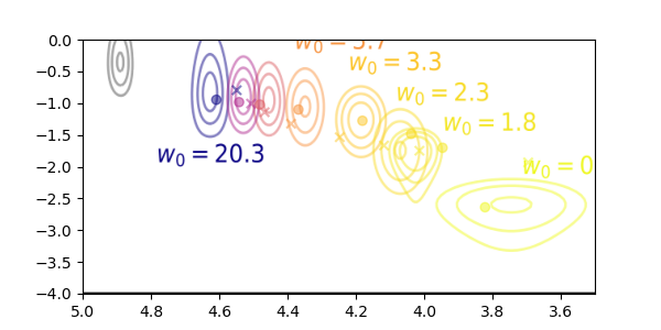
The model of fig. S3 assumes weighted core and shell contributions to the time and to the chemical shift. The values shown here interpolate between a chemical shift of 3.82 for shell water and 4.72 for core water, and between of -2.64 for shell water and -0.89 for core water. The thickness of the shell water that yields this fit is 0.15 nm, notably less that a layer of water, and likely also arguing against the validity of a core-shell model. Also, as noted in the main text, while averaging of relaxation rates () of core vs. shell water molecules represents a physically reasonable situation, averaging of the relaxation times () does not.
Appendix S9 Susceptibility
The susceptibility of different RM solutions varies. On the same day, the relative susceptibility is given by the relative frequencies of the TMS resonance. The absolute susceptibility can be determined by looking at the experiments where a capillary of water with sodium trimethylsilylpropanesulfonate (DSS) was added into the sample. The susceptibility of water is known, allowing us to calculate the exact field, and then the TMS frequency of the RM solution gives the susceptibility of the RM solution.
Appendix S10 A note on proton exchange in glucose
S10.0..1 comment on proton exchange with glucose figure out where to put this – maybe just SI
Because it is a significant recent finding, it is worth discussing that glucose, like other solutes, when encapsulated in reverse micelles (RMs) experiences a decrease in the rate of proton exchange (relative to the rates in bulk aqueous solution) that exhibits a dependence on .sanfordNanoconfinement2016 Initiation of proton exchange is a rare event, but once initiated, it can propagate via standard proton exchange mechanism (e.g., Grotthuss). Assuming that such mechanisms cannot propagate through the aprotic solvent, it’s expected that exchange should be dramatically reduced in reverse micelles for all cases. Regardless, the rates of proton exchange in all cases are expected to be slower than the relaxation rates observed here and, therefore, not to affect the present measurements.
Appendix S11 Relation to Other Types of Measurements
Note that studies of RMs by Dynamic Light Scattering (DLS) have been performed in the past, though have not been repeated here, because we expect the polydispersity measurements by DLS to be similar or weaker reliability compared to the distributions presented here, since both rely on analysis of multivariate exponential decays. Furthermore, DLS is generally considered optimal for larger sized particles and has shown significant discrepancy with the measurements of particle diffusion garnered from Nuclear Magnetic Resonance (NMR) diffusion measurements, which are expected to be quite accurate and more optimal for smaller particle sizes. It is worth noting that significant groundwork has also been laid to relate the present types of measurements to molecular dynamics simulations.Honegger2019NQR
Appendix S12 Low Weight Percent PEG-200
Comparing Aerosol-OT (AOT) RMs in isooctane prepared with a solution of 1 w% PEG-200 to simple solutions of AOT RMs in isooctane, RMs containing PEG-200 exhibit slightly shorter as those without. This indicates a slight reduction in the rotational mobility in the presence of the PEG solution which is expected given the small quantity of PEG added to the solution. Additionally the chemical shifts in the presence of PEG are shifted to slightly lower frequencies. This is indicative of the D2O engaging in less hydrogen bonding to the water matrix, which is again expected as it would be engaging with the PEG molecule. The linewidths with PEG inclusion are slightly larger than those without, which is consistent with the observed slight decrease in .
Appendix S13 Automation and Pulse Program Scripts
S13.1 Automation Program
The automation program (“AU” program) is as follows:
FILE *logfp;char logpath[1000];char titlestr[1000];double peakFreqHz, peakFreqPPM, peakIntensity, maxpsh, maxpsp, maxips, first_maxpsp;double sf, sfo1, o1;float p1;// p1_list should be length-3 array for pulse// lengths around 180 time// nutation_peaks should be length-3 array with// peak intensities (sign matters)// bit for linear regression// pull y-intercept/2 for p1float p1_list[3] = {660.0, 720.0, 780.0};double nutation_peaks[3];int noofscans, pscal_save, i, j, numPeaks;int ns;float repDelay;float my_d1;int stillgoing;#define REAL double#define MIN_DOUBLE 1e-9REAL p1_list_forreg[3];// the following are just function definitions,// with the code given at the bottom, after the quit// statementint linreg(int, const REAL *, const REAL *, REAL *, REAL *, REAL *);void settitle(char *);stillgoing = 1;//{{{ open log fileGETCURDATA; // pulls the info about the foreground // dataset(void)sprintf(logpath, "%s/%s/%d/logfile", disk, name, expno);if ((logfp = fopen(logpath, "wt")) == NULL) { Proc_err(DEF_ERR_OPT, "Can’t open %s\n%s", logpath, strerror(errno)); return 0;}fprintf(logfp, "hello! I am a log file, and I live in expno %d " "-- new version\n", expno);//}}}//{{{ 1H experimentRPAR("ab_1H_zg", "all");fprintf(logfp, "Beginning 1H NMR 1D experiment in %d...\n", expno);RPROCNO(1); // sets procnoSETCURDATA // pull the information for a particular // dataset -- in contrast, // getcurdata pulls the foreground // dataset settitle("NMR experiment w/ standard " "parameters");RGA ZG_OVERWRITE // ERRORABORT returns from AU or AU subroutine // with value of AUERR (if it is less than // 0) there are a couple diff options // (table 2.22 in AU programming manual) ERRORABORT;EF; // FFT w/ exponential apodizationERRORABORT;APK; // auto phase (0 and 1)fprintf(logfp, "Finished 1H NMR 1D experiment.\n");//}}}//{{{ 2H experiment for peak pickingIEXPNO;SETCURDATA; // see comment below about IEXPNOsprintf(titlestr, "2H to find resonance");settitle(titlestr);RPAR("ab_2H_zg", "all");fprintf(logfp, "Beginning 2H NMR 1D experiment for peak " "picking in %d...\n", expno);sf = 0.0;sfo1 = 0.0;o1 = 0.0;p1 = 0.0;//{{{ pull all infoREXPNO(expno);RPROCNO(procno);SETCURDATA//}}}FETCHPAR("SFO1", &sfo1);FETCHPAR("O1", &o1);fprintf(logfp, "here is sfo1: %f\n", sfo1);fprintf(logfp, "here is o1: %f\n", o1);// pull + set number of scansFETCHPAR("NS", &noofscans);fprintf(logfp, "I got %d scans\n", noofscans);ns = 1;STOREPAR("NS", ns);FETCHPAR("NS", &noofscans);fprintf(logfp, "after change, I got %d scans\n", noofscans);// pull + set r.d.FETCHPAR("D1", &repDelay);fprintf(logfp, "I got d1: %f\n", repDelay);my_d1 = 2.5;STOREPAR("D1", my_d1);FETCHPAR("D1", &repDelay);fprintf(logfp, "after change, I got d1: %f\n", repDelay);RGA;ZG_OVERWRITE;ERRORABORT;EF;ERRORABORT;APK;// PSCAL appears to be for vertical scaling. We want to// set// it to "global."FETCHPAR("PSCAL", &pscal_save);STOREPAR("PSCAL", 6);fprintf(logfp, "pscal_save is %d\n", pscal_save);PP; // this tells it to run peak pickingERRORABORT;numPeaks = readPeakList(PROCPATH(0));fprintf(logfp, "I find %d peaks\n", numPeaks);// {{{ store the max peak intensity, frequency, and ppm// in maxip[s,h,p]maxips = 0.0;maxpsh = 0.0;for (i = 0; i < numPeaks; i++) { peakIntensity = getPeakIntensity(i); peakFreqHz = getPeakFreqHz(i); peakFreqPPM = getPeakFreqPPM(i); if (peakIntensity > maxips) { maxips = peakIntensity; maxpsh = peakFreqHz; maxpsp = peakFreqPPM; maxpsp = peakFreqPPM; }}freePeakList();// }}}FETCHPAR("SF", &sf);fprintf(logfp, "I got %f for SF\n", sf);sfo1 = sf + maxpsh * 1.0e-6;fprintf(logfp, "I got %f for SFO1 to set\n", sfo1);STOREPAR("SFO1", sfo1);FETCHPAR("SFO1", &sfo1);FETCHPAR("O1", &o1);FETCHPAR("P1", &p1);fprintf(logfp, "I set SFO1 to %f\n", sfo1);fprintf(logfp, "I set O1 to %f\n", o1);fprintf(logfp, "I set SF to %f\n", sf);fprintf( logfp, "I get P1 of %f (which comes from the par file)\n", p1);// pull + set number of scansFETCHPAR("NS", &noofscans);fprintf(logfp, "I got %d scans\n", noofscans);ns = 1;STOREPAR("NS", ns);FETCHPAR("NS", &noofscans);fprintf(logfp, "after change, I got %d scans\n", noofscans);// pull + set r.d.FETCHPAR("D1", &repDelay);fprintf(logfp, "I got d1: %f\n", repDelay);STOREPAR("D1", my_d1);FETCHPAR("D1", &repDelay);fprintf(logfp, "after change, I got d1: %f\n", repDelay);ZG_OVERWRITE;ERRORABORT;EFP;APK;//}}}// {{{ loop for nutation curvefor (i = 0; i < 3; i++) { if (stillgoing > 0) { fprintf(logfp, "**********************************\n"); fprintf(logfp, "Beginning point %i of nutation curve, the " "experiment " "will be in expno=%d...\n", i, expno + 1); FETCHPAR("P1", &p1); fprintf(logfp, "I had p1 of %f\n", p1); p1 = p1_list[i]; fprintf(logfp, "I want p1 to be %f\n", p1); STOREPAR("P1", p1); FETCHPAR("P1", &p1); fprintf(logfp, "I set p1 to %f\n", p1); // pull + set number of scans FETCHPAR("NS", &noofscans); fprintf(logfp, "I got %d scans\n", noofscans); ns = 1; STOREPAR("NS", ns); FETCHPAR("NS", &noofscans); fprintf(logfp, "after change, I got %d scans\n", noofscans); // pull + set r.d. FETCHPAR("D1", &repDelay); fprintf(logfp, "I got d1: %f\n", repDelay); STOREPAR("D1", my_d1); FETCHPAR("D1", &repDelay); fprintf(logfp, "after change, I got d1: %f\n", repDelay); IEXPNO; SETCURDATA; // pg 15 -- IEXPNO changes current // dataset, but doesn’t // "make it available" -- must be // followed by SETCURDATA for other // commands that access the current // dataset (I believe that here that // includes our settitle function) // {{{ set processing params and title unique to // nutation sprintf(titlestr, "nutation step %d", i); settitle(titlestr); STOREPAR("LB", 5.0); STOREPAR("PSIGN", 2); // "both" // }}} ZG_OVERWRITE; EFP // exp FT and apply PHC0 and PHC1 -- don’t think // it alters PHC0 and PHC1 if (i == 0){ APK // this alters PHC0 and PHC1 } FETCHPAR("PSCAL", &pscal_save); STOREPAR("PSCAL", 6); fprintf(logfp, "pscal_save is %d\n", pscal_save); PP; // peak pick ERRORABORT; numPeaks = readPeakList(PROCPATH(0)); fprintf(logfp, "I find %d peaks\n", numPeaks); // store the max peak intensity, frequency, and ppm // in maxip[s,h,p] maxips = 0.0; maxpsh = 0.0; for (j = 0; j < numPeaks; j++) { peakIntensity = getPeakIntensity(j); peakFreqHz = getPeakFreqHz(j); peakFreqPPM = getPeakFreqPPM(j); fprintf(logfp, "check peak intensity %f at %f\n", peakIntensity, peakFreqPPM); fprintf(logfp, "comparing %f to %f\n", abs(peakIntensity), abs(maxips)); if (abs(peakIntensity) > abs(maxips)) { maxips = peakIntensity; maxpsh = peakFreqHz; maxpsp = peakFreqPPM; } } if (i == 0) { first_maxpsp = maxpsp; } else { if (abs(first_maxpsp - maxpsp) > 1.0) { fprintf(logfp, "I’m exiting because the " "frequency deviation " "is too large\n"); stillgoing = 0; } } } if (stillgoing > 0) { fprintf(logfp, "for nutation step %d, the peak parameters " "are ips=%f " "psh=%f psp=%f\n", i, maxips, maxpsh, maxpsp); freePeakList(); fprintf(logfp, "For my first nutation, I set p1 to %f\n", p1); fprintf( logfp, "For my first nutation, I get peak max of %f\n", maxips); nutation_peaks[i] = maxips; }}// }}}// {{{ find the 90 time from the list of 3 peaksif (stillgoing > 0) { fprintf(logfp, "*** *** *** *** *** *** *** *** ***\n"); fprintf(logfp, "result of nutation curve:\n"); for (i = 0; i < 3; i++) { fprintf(logfp, "p1=%f\theight=%f\n", p1_list[i], nutation_peaks[i]); } if (nutation_peaks[2] > 0) { fprintf(logfp, "I’m going to quit b/c the 3rd " "nutation peak is positive!\n"); stillgoing = 0; }}if (stillgoing > 0) { REAL m, b, r2; for (i = 0; i < 3; i++) { p1_list_forreg[i] = (REAL)p1_list[i]; } linreg(3, p1_list_forreg, nutation_peaks, &m, &b, &r2); p1 = -b / m / 2.; IEXPNO; fprintf(logfp, "m=%f b=%f r=%g\n", m, b, r2); fprintf(logfp, "going to set p1 to %f in %d\n", p1, expno); STOREPAR("P1", p1); ZG_OVERWRITE; ERRORABORT; EFP; APK; if (p1 > 800 || p1 < 0) { fprintf(logfp, "that’s an invalid value for " "p1!!!\nI’m going to quit!!!\n"); STOREPAR("P1", 360.0); stillgoing = 0; }}// }}}if (stillgoing) { //{{{ 2H IR IEXPNO SETCURDATA fprintf(logfp, "**********************************\n"); fprintf(logfp, "Incrementing experiment number to %d...\n", expno); RPAR("ab_2H_T1_logSpace", "all"); STOREPAR("SFO1", sfo1); STOREPAR("O1", o1); FETCHPAR("SFO1", &sfo1); FETCHPAR("O1", &o1); fprintf(logfp, "In IR expjeriment, I set SFO1 to %f\n", sfo1); fprintf(logfp, "In IR experiment, I set O1 to %f\n", o1); FETCHPAR1("SFO1", &sfo1); FETCHPAR1("O1", &o1); fprintf( logfp, "In IR experiment, I have SFO1 (indirect) as %f\n", sfo1); fprintf( logfp, "In IR experiment, I have O1 (indirect) as %f\n", o1); STOREPAR("P1", p1); fprintf(logfp, "In IR experiment, I set P1 to %f\n", p1); FETCHPAR("P1", &p1); fprintf(logfp, "In IR experiment, I get P1 of %f\n", p1); // pull + set r.d. FETCHPAR("D1", &repDelay); fprintf(logfp, "I got d1: %f\n", repDelay); STOREPAR("D1", my_d1); FETCHPAR("D1", &repDelay); fprintf(logfp, "after change, I got d1: %f\n", repDelay); ZG_OVERWRITE; //}}}}// close downfclose(logfp);QUIT// the above code relies on some standard C functions,// which rely on other (standard) headers: these are// defined here.//// Note that we do need to include the function// declarations at the top of the AU file, as well.#include <math.h>#include <stdlib.h> inline static REAL sqr(REAL x) { return x * x;}// linear regression functionint linreg(int n, const REAL x[], const REAL y[], REAL *m, REAL *b, REAL *r) { REAL sumx = 0.0; /* sum of x */ REAL sumx2 = 0.0; /* sum of x**2 */ REAL sumxy = 0.0; /* sum of x*y */ REAL sumy = 0.0; /* sum of y */ REAL sumy2 = 0.0; /* sum of y**2 */ int i; for (i = 0; i < n; i++) { sumx += x[i]; sumx2 += sqr(x[i]); sumxy += x[i] * y[i]; sumy += y[i]; sumy2 += sqr(y[i]); } REAL denom = (n * sumx2 - sqr(sumx)); if (denom == 0) { // singular matrix. can’t solve the problem. *m = 0; *b = 0; if (r) *r = 0; return 1; } *m = (n * sumxy - sumx * sumy) / denom; *b = (sumy * sumx2 - sumx * sumxy) / denom; if (r != NULL) { *r = (sumxy - sumx * sumy / n) / /* compute correlation coeff */ sqrt((sumx2 - sqr(sumx) / n) * (sumy2 - sqr(sumy) / n)); double slope = ((n * sumxy) - (sumx * sumy)) / denom; double intercept = ((sumy * sumx2) - (sumx * sumxy)) / denom; double term1 = ((n * sumxy) - (sumx * sumy)); double term2 = ((n * sumx2) - (sumx * sumy)); double term3 = ((n * sumy2) - (sumy * sumy)); double term23 = (term2 * term3); double r2 = 1.0; if (fabs(term23) > MIN_DOUBLE) r2 = (term1 * term1) / term23; } return 0;}void settitle(char *string) { char titlename[1000]; FILE *titlefp; (void)sprintf(titlename, "%s/%s/%d/pdata/%d/title", disk, name, expno, procno); if ((titlefp = fopen(titlename, "wt")) == NULL) { Proc_err(DEF_ERR_OPT, "Can’t open %s\n%s", titlename, strerror(errno)); return 0; } fprintf(titlefp, string); fclose(titlefp);}
S13.2 Pulse Program
The pulse program is a standard inversion recovery, but employs (1) utilization of the lock channel for acquisition and (2) separately stored phase cycles following the recipe given previously.beatonModernized2022
;ab_IR2h (written aug2020);based off egr_IR;avance-version (12/01/11);1D sequence;using 2H lockswitch unit or BSMS 2H-TX board;;$CLASS=HighRes;$DIM=1D;$TYPE=;$SUBTYPE=;$COMMENT=#include<Avance.incl>#include<Sysconf.incl>define loopcounter total_ph_steps"p2=p1*2""d11=30m""acqt0=-p1*2/3.1416""l20=2" ;steps in ph1"l21=4" ;steps in ph2"total_ph_steps = l20*l21""l23=td1/total_ph_steps";td1=number of phase steps * vdlist;td2=40961 ze d11 LOCKDEC_ON d11 H2_PULSE2 30m rpp1 1m rpp23 30m H2_LOCK d1 d11 H2_PULSE p2:D ph1 vd p1:D ph2 goscnp ph31 d11 wr #0 if #0 2u ipp2 lo to 3 times l21 2u ipp1 lo to 3 times l20 0.1u ivd lo to 2 times l23 d11 H2_LOCK d11 LOCKDEC_OFFexitph1=0 2ph2=0 1 2 3ph31=0;pl1 : f1 channel - power level for pulse (default);p1 : f1 channel - 90 degree high power pulse;d1 : relaxation delay; 1-5 * T1;d11: delay for disk I/O [30 msec];ns: 1 * n, total number of scans: NS * TD0;locnuc: off;$Id: zg2h,v 1.14.8.1 2012/01/31 17:56:41 ber Exp $
Appendix S14 Inverse Laplace Transform
A PDF export of an explanatory jupyter notebook that converts raw data from these programs to a correlated distribution of vs. chemical shift is attached at the end of this supporting information document. (The data in the resulting HDF file is read into subsequent scripts that compile and display contours from multiple experiments.)
References
- (1) M. Ueda and Z. A. Schelly. “Mean aggregation number and water vapor pressure of AOT reverse micellar systems determined by controlled partial pressure-vapor pressure osmometry (CPP-VPO).” Langmuir, 4(3):653–655 (1988). doi:10.1021/la00081a026.
- (2) H.-F. Eicke. “Surfactants in nonpolar solvents.” In “Micelles,” volume 87, pages 85–145. Springer-Verlag, Berlin/Heidelberg (1980). ISBN 978-3-540-09639-9.
- (3) I. R. Piletic, D. E. Moilanen, D. B. Spry, N. E. Levinger, and M. D. Fayer. “Testing the Core/Shell Model of Nanoconfined Water in Reverse Micelles Using Linear and Nonlinear IR Spectroscopy.” J. Phys. Chem. A, 110(15):4985–4999 (2006). doi:10.1021/jp061065c.
- (4) A. Abragam. The Principles of Nuclear Magnetism, pages 314–315. Clarendon Press (1961). ISBN 978-0-19-852014-6. Google-Books-ID: 9M8U_JK7K54C.
- (5) C. P. Slichter. Principles of Magnetic Resonance, pages 163–171. Springer-Verlag, third edition (1989).
- (6) B. P. Wiebenga-Sanford, J. DiVerdi, C. D. Rithner, and N. E. Levinger. “Nanoconfinement’s Dramatic Impact on Proton Exchange between Glucose and Water.” J. Phys. Chem. Lett., 7(22):4597–4601 (2016). doi:10.1021/acs.jpclett.6b01651.
- (7) P. Honegger and O. Steinhauser. “Hydration dynamics of proteins in reverse micelles probed by 1 H-NOESY/ 1 H-ROESY NMR and 17 O-nuclear quadrupole resonance (NQR).” Phys. Chem. Chem. Phys., 21(27):14571–14582 (2019). PMID: 31237595. doi:10.1039/C9CP02654A.
- (8) A. A. Beaton, A. Guinness, and J. M. Franck. “A modernized view of coherence pathways applied to magnetic resonance experiments in unstable, inhomogeneous fields.” J. Chem. Phys., 157(17):174204 (2022). doi:10.1063/5.0105388.