Conformalizing Machine Translation Evaluation
Abstract
Several uncertainty estimation methods have been recently proposed for machine translation evaluation. While these methods can provide a useful indication of when not to trust model predictions, we show in this paper that the majority of them tend to underestimate model uncertainty, and as a result they often produce misleading confidence intervals that do not cover the ground truth. We propose as an alternative the use of conformal prediction, a distribution-free method to obtain confidence intervals with a theoretically established guarantee on coverage. First, we demonstrate that split conformal prediction can “correct” the confidence intervals of previous methods to yield a desired coverage level. Then, we highlight biases in estimated confidence intervals, both in terms of the translation language pairs and the quality of translations. We apply conditional conformal prediction techniques to obtain calibration subsets for each data subgroup, leading to equalized coverage.
1 Introduction
Neural models for natural language processing (NLP) are able to tackle increasingly challenging tasks with impressive performance. However, their deployment in real world applications does not come without risks. For example, systems that generate fluent text might mislead users with fabricated facts, particularly if they do not expose their confidence. High performance does not guarantee an accurate prediction for every instance—and even less so when an instance is noisy or out of distribution—which makes uncertainty quantification methods more important than ever.
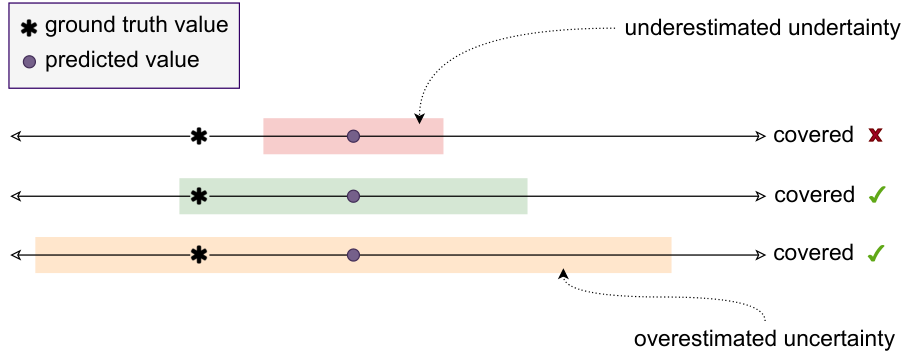
While most work on uncertainty estimation for NLP has focused on classification tasks, uncertainty quantification for text regression tasks, uncertainty quantification has recently gained traction for text regression tasks, such as machine translation (MT) evaluation, semantic sentence similarity, or sentiment analysis Wang et al. 2022; Glushkova et al. 2021. A wide range of methods have been proposed for estimating uncertainty in regression, the majority of which involve underlying assumptions on the distribution or the source of uncertainty Kendall and Gal 2017a; Kuleshov et al. 2018a; Amini et al. 2020; Ulmer et al. 2023. However, it has been shown that such assumptions are often unrealistic and may lead to misleading results Izmailov et al. 2021; Zerva et al. 2022. More importantly, most commonly used methods provide confidence intervals without any theoretically established guarantees with respect to coverage. In other words, while a representative confidence interval should include (cover) the ground truth target value for each instance (and ideally the bound of the confidence interval should be close to the ground truth as shown in Figure 2), frequently the predicted interval is much narrower, excluding the ground truth and underestimating the model uncertainty. In fact, for the concrete problem of MT evaluation, we show that the majority of uncertainty quantification methods achieve very low coverage even after calibration, as can be observed in Figure 2. Finally, it has been shown that while uncertainty quantification can shed light on model weaknesses and biases, the uncertainty prediction methods themselves can suffer from biases and provide unfair and misleading predictions for specific data subgroups or for examples with varying levels of difficulty Cherian and Candès 2023; Ding et al. 2020; Boström and Johansson 2020.
To address the aforementioned shortcomings, we explore the use of conformal prediction as a means to obtain more trustworthy confidence intervals on textual regression tasks, using MT evaluation as the primary paradigm. We rely on the fact that given a scoring or uncertainty estimation function, conformal prediction can provide statistically rigorous uncertainty intervals for regression models Angelopoulos and Bates 2021; Vovk et al. 2005; Vovk et al. 2022. More importantly, the conformal prediction methodology provides theoretical guarantees about coverage over a test set, given a chosen coverage threshold. The predicted uncertainty intervals are thus valid in a distribution-free sense: they possess explicit, non-asymptotic guarantees even without distributional assumptions or model assumptions Angelopoulos and Bates 2021; Vovk et al. 2005.
We specifically show that previously proposed uncertainty quantification methods can be used to design non-conformity scores for split conformal prediction Papadopoulos 2008. We demonstrate that, regardless of the initially obtained coverage, the application of conformal prediction can increase coverage to the desired —user defined— value (see Figure 2). To this end, we compare four parametric uncertainty estimation methods (Monte Carlo dropout, deep ensembles, heteroscedastic regression, and direct uncertainty prediction) and one non-parametric method (quantile regression) with respect to coverage and distribution of uncertainty intervals.
Moreover, we investigate the fairness of obtained intervals for two different attributes: (1) translation language pair; and (2) translation difficulty, as reflected by human quality estimates. We highlight unbalanced coverage for both cases and demonstrate how conditional conformal prediction Angelopoulos and Bates 2021; Boström and Johansson 2020; Boström et al. 2021 can address such imbalances effectively.
2 Conformal Prediction
In this section, we provide background on conformal prediction and introduce the notation used throughout this paper. Later in §3 we show how this framework can be used for uncertainty quantification in MT evaluation.
2.1 Desiderata
Let and be random variables representing inputs and outputs, respectively; in this paper we focus on regression, where . We use upper case to denote random variables and lower case to denote their specific values. Traditional machine learning systems use training data to learn predictors which, when given a new test input , output a point estimate . However, such point estimates lack uncertainty information. Conformal prediction Vovk et al. 2005, in contrast, considers set functions , providing the methodology for, given , returning a prediction set with theoretically established guarantees regarding the coverage of the ground truth value. For regression tasks, this prediction set is usually a confidence interval (see Figure 2). Conformal prediction techniques have recently proved useful in many applications: for example, in the U.S. presidential election in 2020, the Washington Post used conformal prediction to estimate the number of outstanding votes (Cherian and Bronner 2020).
Given a desired confidence level (e.g. 90%), these methods have a formal guarantee that, in expectation, contains the true value with a probability equal to or higher than the given confidence level. Importantly, this is done in a distribution-free manner, i.e., without making any assumptions on the data distribution beyond exchangeability, a weaker assumption than independent and identically distributed (i.i.d.) data.11 1 Namely, the data distribution is said to be exchangeable iff, for any sample and any permutation function , we have . If the data distribution is i.i.d., then it is automatically exchangeable, since and the product of scalars is commutative. By de Finetti’s theorem (De Finetti 1929), exchangeable observations are conditionally independent relative to some latent variable.
In this paper, we use a simple inductive method called split conformal prediction Papadopoulos 2008, which requires the following ingredients:
- •
A mechanism to obtain non-conformity scores for each instance, i.e., a way to estimate how “unexpected” an instance is with respect to the rest of the data. In this work, we do this by leveraging a pretrained predictor together with some heuristic notion of uncertainty—our method is completely agnostic about which model is used for this. We describe in §2.2 the non-conformity scores we design in our work.
- •
A held-out calibration set containing examples, . The underlying distribution from which the calibration set is generated is assumed unknown but it must be exchangeable (see footnote 1).
- •
A desired error rate (e.g. ), such that the coverage level will be (e.g. 90%).
These ingredients are used to generate prediction sets for new test inputs. Specifically, let be the non-conformity scores of each example in the calibration set, i.e., . Define as the empirical quantile of these non-conformity scores, where is the ceiling function. This quantile can be easily obtained by sorting the non-conformity scores and examining the tail of the sequence. Then, for a new test input , we output the prediction set
| (1) |
We say that coverage holds if the true output lies in the prediction set, i.e., . This simple procedure has the following theoretical coverage guarantee:
Theorem 1 (Vovk et al. 1999; Vovk et al. 2005)
Using the above quantities, the following bounds hold:
This result tells us two important things: (i) the expected coverage is at least , and (ii) with a large enough calibration set (large ), the procedure outlined above does not overestimate the coverage too much, so we can expect it to be nearly .22 2 For most purposes, a reasonable size for the calibration set is . See Angelopoulos and Bates 2021.
2.2 Non-conformity scores
Naturally, the result stated in Theorem 1 is only practically useful if the prediction sets are small enough to be informative—to ensure this, we need a good heuristic to generate the non-conformity scores. In this paper, we are concerned with regression problems (), so we define the prediction sets to be confidence intervals. We assume we have a pretrained regressor , and we consider two scenarios, one where we generate symmetric intervals (i.e., where is the midpoint of the interval) and a more general scenario where intervals can be non-symmetric.
Symmetric intervals.
In this simpler scenario, we assume that, along with , we have a corresponding uncertainty heuristic , where higher values signify higher uncertainty. An example—to be elaborated upon in §3.2.1—is where is the quantile of a symmetric probability density, such as a Gaussian, which can be computed analytically from the variance. We then define the non-conformity scores as
| (2) |
and follow the procedure above to obtain the quantile from the calibration set. Then, for a random test point and from (1) and (2), we have:
| (3) |
which corresponds to the confidence interval
| (4) |
We examine this procedure in §3.2.1 with various uncertainty heuristics (Monte Carlo dropout, deep ensembles, heteroscedastic regression, and direct uncertainty prediction estimates).
Non-symmetric intervals.
Sometimes, better heuristics can be obtained which are non symmetric, i.e., where there is larger uncertainty in one of the sides of the interval—we will see a concrete example in §3.2.2 where we describe a non-parametric quantile regression procedure (although this might happen as well with parametric heuristics based on fitting non-symmetric distributions, such as the skewed beta distribution). In this case, we assume left and right uncertainty estimates and , both non-negative and satisfying , and define the non-conformity scores as:
This leads to prediction sets
| (7) |
which also satisfy Theorem 1. Naturally, when , this procedure recovers the symmetric case.
3 Conformal MT Evaluation
We now apply the machinery of conformal prediction to the problem of MT evaluation, experimenting with a range of uncertainty quantification heuristics to generate and (or and in the non-symmetric case).
In MT evaluation, the input is a triplet of source, automatic translation, and human reference segment, , and the goal is to predict a scalar value that corresponds to the estimated quality of the translation . The ground truth is a quality score manually produced by a human annotator, called a direct assessment (DA) (Graham 2013). We use DA scores that are standardised for each annotator. An example instance is shown in Figure 3.
We describe our datasets and experimental setup in §3.1. With the application of symmetric parametric uncertainty methods, described in §3.2.1, we obtain heuristics and which we use to obtain non-conformity scores via (2), leading to the confidence intervals in (4), for each triplet. Alternatively, in §3.2.2 we describe a non-symmetric and non-parametric method which returns , , and , and which we will use to compute the non-conformity scores (2.2) and confidence intervals (7).
3.1 Experimental setup
Model.
We use Comet as the underlying MT quality evaluation model (Rei et al. 2020). We train the Comet model using a pretrained XLM-RoBERTa-Large encoder fine-tuned for 2 epochs with the default training configurations.33 3 More precisely, we used the wmt-large-da-estimator-1719 available at: https://unbabel.github.io/COMET/html/models.html.
Data.
For training, we use the direct assessment (DA) data from the WMT17-19 metrics shared tasks Ma et al. 2018; Ma et al. 2019. We evaluate our models on the WMT20 metrics dataset Mathur et al. 2020. For the calibration set , we use repeated random sub-sampling for runs. The WMT20 test data includes 16 language pairs, of which 9 pairs are into-English and 7 pairs are out-of-English translations. For the calibration set sub-sampling, we sample uniformly from each language pair. For metrics for which we report averaged performance we use micro-average over all language pairs.
3.2 Uncertainty quantification methods
We experiment with a diverse set of uncertainty prediction methods, accounting both for parametric and non-parametric uncertainty prediction. We extensively compare all the parametric methods previously used in MT evaluation (Zerva et al. 2022), which return symmetric confidence intervals, and also experiment with quantile regression Koenker and Hallock 2001, a simple non-parametric approach that has never been used for MT evaluation, and which can return non-symmetric intervals.
3.2.1 Parametric uncertainty
We compare a set of different parametric methods which fit the quality scores in the training data to an input-dependent Gaussian distribution . All these methods lead to symmetric confidence intervals (see Eq. 4). We use these methods to obtain estimates . Then we use to extract the corresponding uncertainty estimates as , which correspond to the and quantiles of the Gaussian, for a given confidence threshold . For (i.e., a 90% confidence level) this results in . We describe the concrete methods used to estimate and below.
MC dropout (MCD).
This is a variational inference technique approximating a Bayesian network with a Bernoulli prior distribution over its weights Gal and Ghahramani 2016. By retaining dropout layers during multiple inference runs, we can sample from the posterior distribution over the weights. As such, we can approximate the uncertainty over a test instance through a Gaussian distribution with the empirical mean and variance of the quality estimates . We use 100 runs, following the analysis of Glushkova et al. 2021.
Deep ensembles (DE).
This method Lakshminarayanan et al. 2017 trains an ensemble of neural models with the same architecture but different initializations. During inference, we collect the predictions of each single model and return and as in MC dropout. We use checkpoints obtained with different initialization seeds, following Glushkova et al. 2021.
Heteroscedastic regression (HTS).
We follow Le et al. 2005 and Kendall and Gal 2017b and incorporate as part of the training objective. This way, a regressor is trained to output two values: (1) a mean score and (2) a variance score . This predicted mean and variance parameterize a Gaussian distribution , where are the model parameters. The negative log-likelihood loss function is used:
| (8) |
This framework is particularly suitable to express aleatoric uncertainty due to heteroscedastic noise, as the framework allows larger variance to be assigned to “noisy” examples which will have the effect of downweighting the squared term in the loss.
Direct uncertainty prediction (DUP).
This is a two-step procedure which relies on the assumption that the total uncertainty over a test instance is equivalent to the generalization error of the regression model Lahlou et al. 2021. A standard regression model is first fit on the training set and then applied to a held-out validation set . Then, a second model is trained on this held-out set to regress on the error incurred by the first model predictions, approximating its uncertainty. To train the error predicting model, we follow the setup of Zerva et al. 2022, using as inputs the triplets combined with the predictions of first model, which are used as bottleneck features in an intermediate fusion fashion. The loss function is
| (9) |
We use as the uncertainty heuristic.
3.2.2 Non-parametric uncertainty: Quantile regression (QNT)
Quantile regression is a statistical method used to model input-dependent quantiles within a regression framework (Koenker and Bassett Jr 1978). As opposed to regular (linear) regression that models the mean of a target variable conditioned on the input , quantile regression models a quantile of the distribution of (e.g. the median, the 95%, or the 5% percentile scores). By definition, quantile regression does not require any parametric assumptions on the distribution of and is less sensitive to outliers. Quantiles provide an attractive representation for uncertainty: they allow for easy construction of prediction intervals, at chosen confidence levels. Learning the quantile for a particular quantile level involves optimizing the pinball loss, a tilted transformation of the absolute value function (see Figure 4). Given a target , a prediction , and quantile level , the pinball loss is defined as:
| (10) |
We can select to correspond to the error rate that we want to achieve. Note that for the the loss function reduces to (half) the mean absolute error loss .
We use to train our models to predict the and quantiles, as well as the quantile, which corresponds to the median (see below), but there are extensions that either optimize multiple quantiles that cover the full predictive distribution Tagasovska and Lopez-Paz 2019 or explore asymmetric loss extensions to account for overestimating or underestimating the confidence intervals Beck et al. 2016.
Unlike the parametric methods covered in §3.2.1, the quantile regression method can be used to return asymmetric confidence intervals. This is done by fitting 0.5, , and quantile predictors to the data, and setting , , and .
For completeness, we also consider a symmetric variant of quantile regression where we do not estimate the median , but rather set . We report coverage for both the non-symmetric (QNT-NS) and the symmetric case (QNT-S) later in Table 1.
3.3 Comparison with calibration
We also compare the coverage obtained by uncertainty methods and conformal prediction to a calibration approach that aims to minimize the expected calibration error (ECE; Naeini et al. 2015; Kuleshov et al. 2018b). ECE has been proposed as a measure of how well aligned the model confidence is with the model accuracy, based on the simple desideratum that a model with e.g. 80% confidence over a set of examples should achieve an accuracy of 80% over the same examples to be well-calibrated. It is defined as
| (11) |
where each is a bin representing a confidence level , and is the fraction of times the ground truth falls inside the confidence interval associated to that bin. Several variants of uncertainty calibration have been proposed to correct unreliable uncertainty estimates that do not correlate with model accuracy Kuleshov et al. 2018b; Amini et al. 2020; Levi et al. 2022. We follow Glushkova et al. 2021 who find that computing a simple affine transformation of the original uncertainty distribution that minimises the ECE is effective to quantify uncertainty in MT evaluation.
3.4 Results
We first compare the uncertainty methods described in §3.2 with respect to coverage percentage as shown in Table 1. We select a desired coverage level of , i.e., we set . We also align the uncertainty estimates with respect to the same value: for the parametric uncertainty heuristics, we select the that corresponds to a coverage of the distribution, by using the probit function as described in §3.2.1; and for the non-parametric approach, we train the quantile regressors by setting , as described in §3.2.2.
| Method | Orig. | Calib. | Conform. | |
|---|---|---|---|---|
| QNT-NS | 77.83 | – | 90.21 | 1.44 |
| QNT-S | 78.66 | 69.03 | 90.54 | 1.41 |
| MCD | 23.82 | 66.60 | 90.01 | 8.01 |
| DE | 29.10 | 66.23 | 91.31 | 7.06 |
| HTS | 82.18 | 68.29 | 89.89 | 1.31 |
| DUP | 86.23 | 66.13 | 89.88 | 1.14 |
Table 1 shows that coverage varies significantly across methods, with the sampling-based methods such as MC dropout and deep ensembles achieving coverage much below the desired level. In contrast, direct uncertainty prediction achieves comparatively high coverage even before the application of conformal prediction. This could be related to the fact that by definition, the DUP method tries to predict uncertainty modeled as .
Calibration helps improve coverage in the cases of MC dropout and deep ensembles—albeit still without reaching close to 0.9. Instead, it seems that minimizing the ECE is not well aligned to optimizing coverage as for all cases calibration leads to less than coverage. In contrast, we can see that conformal prediction approximates the desired coverage level best for all methods, regardless of the initial coverage they obtain, in line with the guarantees provided by Theorem 1.
Besides measuring the coverage achieved by the several methods, it is also important to examine the width of the predicted intervals—if intervals are too wide, they will not be very informative nor useful in practice (see also Figure 2). To that end, we also compute the sharpness (Kuleshov and Deshpande 2022) as the average width of the predicted confidence intervals after the conformal prediction application 44 4 In related work Glushkova et al. 2021 sharpness is computed with respect to , but this cannot be applied to non-parametric uncertainty cases, so we use the confidence interval length to be able to compare conformal prediction for all uncertainty quantification methods.,
| (12) |
We show the results in Table 2. We observe that, for the majority of methods, the sharpness values are similar, except for deep ensembles (DE) where we need to rely on wider intervals to achieve the same level of coverage.
| Method | Sharpness |
|---|---|
| QNT-NS/S | 2.409 |
| MCD | 2.629 |
| DE | 3.074 |
| HTS | 2.304 |
| DUP | 2.486 |
4 Conditional Coverage
The coverage guarantees stated in Theorem 1 refer to marginal coverage—the probabilities are not conditioned on the input points, they are averaged (marginalized) over the full test set. In several practical situations it is desirable to assess the conditonal coverage where denotes a region of the input space, e.g., inputs containing some specific attributes or pertaining to some group of the population.
In fact, evaluating the conditional coverage with respect to different data attributes may reveal biases of the uncertainty estimation methods towards specific data subgroups which are missed if we only consider marginal coverage. In the next experiments, we follow the feature stratified coverage described in Angelopoulos and Bates 2021; we use conformal prediction with MC dropout as our main paradigm where MC dropout is used as the underlying uncertainty quantification method. We demonstrate three examples of imbalanced coverage in Figure 6 with respect to three different attributes: language pairs, translation quality level, and estimated uncertainty scores.
We can see that, in all cases, coverage varies significantly across groups, revealing biases towards specific attribute values. For example, the plots show that into-English translations are under-covered (coverage ), i.e., we consistently underestimate the uncertainty over the predicted quality for these language pairs. More importantly, we can see that examples with low translation quality (measured by human scores) are significantly under-covered, as coverage for quality scores where drops below 50%. Observing the frequencies of these segments, we can see that the drop in segment frequency seems to correlate with a significant drop in coverage. For MCD-based uncertainty scores on the other hand, the drop in coverage seems to be related to the low uncertainty scores, indicating that due to the skewed distribution of uncertainty scores, the calculation of the quantile is not well tuned to lower uncertainty values (i.e., higher non-conformity scores). Similar patterns for these three dimensions are also observed for the other uncertainty quantification methods revealing the biases of these methods.
Ensuring we do not overestimate confidence for these examples (specially for low quality segments) is crucial for MT evaluation, in particular for applications where MT is used on the fly and one needs to know if a translation can be shared or would require further editing with human intervention. Hence, in the rest of this section, we elaborate approaches to assess and mitigate coverage imbalance in the aforementioned examples, in order to obtain more equalized coverage Romano et al. 2020. We consider conditional coverage both for discrete (language pairs) and continuous (quality scores) attributes.
4.1 Conditioning on discrete attributes: language-pairs
To deal with imbalanced coverage for discrete data attributes, such as the language pair, we use an equalized conformal prediction approach, i.e., we compute the conditional coverage for each attribute value and, upon observing imbalances, we compute conditional quantiles instead of a single one on the calibration set.
Let index the several attributes (e.g., language pairs). We partition the calibration set according to these attributes, , where denotes the partition corresponding to the th attribute and for every . Then, we follow the procedure described in §2 to fit attribute-specific quantiles to each calibration set .
We demonstrate the application of this process on language pairs for all uncertainty quantification methods examined in the previous section. Table 3 shows the language-based conditional coverage, using a heatmap coloring to highlight the language pairs that fall below the guaranteed marginal coverage of . We can see that for all language pairs we achieve coverage >75% but some are below the 90% target. For all methods except for DUP, the coverage is high for out-of-English translations and drops for the majority of into-English cases. Instead, DUP seems to be the method obtaining the most balanced performance across languages, with smaller deviations that do not seem to favor a specific translation direction. Applying the equalizing approach described above, we successfully rectify the imbalance for all uncertainty quantification methods, as shown in the heatmap of Table 4.
| QNT | MCD | DE | HTS | DUP | |
|---|---|---|---|---|---|
| En-Cs | 0.982 | 0.959 | 0.939 | 0.875 | 0.931 |
| En-De | 0.973 | 0.971 | 0.925 | 0.863 | 0.927 |
| En-Ja | 0.990 | 0.978 | 0.987 | 0.886 | 0.972 |
| En-Pl | 0.977 | 0.948 | 0.914 | 0.882 | 0.914 |
| En-Ru | 0.974 | 0.958 | 0.936 | 0.862 | 0.926 |
| En-Ta | 0.970 | 0.952 | 0.949 | 0.892 | 0.858 |
| En-Zh | 0.934 | 0.983 | 0.991 | 0.919 | 0.945 |
| Cs-En | 0.890 | 0.871 | 0.884 | 0.898 | 0.875 |
| De-En | 0.880 | 0.888 | 0.867 | 0.896 | 0.902 |
| Ja-En | 0.883 | 0.856 | 0.921 | 0.910 | 0.887 |
| Kn-En | 0.881 | 0.875 | 0.948 | 0.943 | 0.840 |
| Pl-En | 0.862 | 0.833 | 0.825 | 0.873 | 0.849 |
| Ps-En | 0.851 | 0.854 | 0.932 | 0.922 | 0.786 |
| Ru-En | 0.851 | 0.828 | 0.831 | 0.879 | 0.888 |
| Ta-En | 0.793 | 0.809 | 0.878 | 0.898 | 0.883 |
| Zh-En | 0.861 | 0.833 | 0.868 | 0.886 | 0.827 |
| QNT | MCD | DE | HTS | DUP | |
|---|---|---|---|---|---|
| En-Cs | 0.893 | 0.917 | 0.888 | 0.892 | 0.902 |
| En-De | 0.902 | 0.902 | 0.902 | 0.896 | 0.893 |
| En-Ja | 0.909 | 0.891 | 0.900 | 0.891 | 0.904 |
| En-Pl | 0.882 | 0.905 | 0.895 | 0.900 | 0.898 |
| En-Ru | 0.900 | 0.898 | 0.908 | 0.906 | 0.903 |
| En-Ta | 0.903 | 0.895 | 0.883 | 0.886 | 0.903 |
| En-Zh | 0.880 | 0.890 | 0.884 | 0.896 | 0.896 |
| Cs-En | 0.890 | 0.917 | 0.909 | 0.904 | 0.894 |
| De-En | 0.897 | 0.901 | 0.901 | 0.897 | 0.903 |
| Ja-En | 0.900 | 0.912 | 0.899 | 0.894 | 0.902 |
| Kn-En | 0.896 | 0.903 | 0.902 | 0.904 | 0.894 |
| Pl-En | 0.900 | 0.905 | 0.893 | 0.894 | 0.877 |
| Ps-En | 0.905 | 0.899 | 0.900 | 0.884 | 0.907 |
| Ru-En | 0.910 | 0.896 | 0.907 | 0.900 | 0.900 |
| Ta-En | 0.884 | 0.901 | 0.886 | 0.901 | 0.908 |
| Zh-En | 0.900 | 0.910 | 0.908 | 0.900 | 0.905 |
4.2 Conditioning on continuous attributes: translation quality and uncertainty scores
With some additional constraints on the equalized conformal prediction process described in §4.1 we can generalize this approach to account for attributes with continuous values, such as the quality scores (ground truth quality ) in the case of MT evaluation or the uncertainty scores obtained by different uncertainty quantification methods. To that end, we adapt the Mondrian conformal prediction methodology Vovk et al. 2005. Mondrian conformal predictors have been used initially for classification and later for regression, where they have been used to partition the data with respect to the residuals Johansson et al. 2014. Boström and Johansson 2020 proposed a Mondrian conformal predictor that partitions along the expected “difficulty” of the data as estimated by the non-conformity score or the uncertainty score .
In all the above cases, the calibration instances are sorted according to continuous variable of interest and then partitioned into calibration bins. While the bins do not need to be of equal size, they need to satisfy a minimum length condition that depends on the chosen threshold for the error rate Johansson et al. 2014. Upon obtaining a partition into calibration bins, and similarly to what was described in §4.1 for discrete attributes, we compute bin-specific quantiles , where indexes a bin.
We apply the aforementioned approach to the MT evaluation for the translation quality scores as well as the predicted uncertainty scores. For both cases, we set a threshold of at least segments per bin. For the translation quality scores, we initially compute quality score bins and quantiles over the calibration set using the ground truth scores as described previously. Subsequently, to apply the conformal prediction on a test instance , we use the predicted quality score and choose the best bin to use by computing the smallest difference between and the mean quality score of the calibration bins. We then predict the confidence interval by using the corresponding quantile . For the uncertainty scores, the application is easier, since we have access to the uncertainty prediction for both the calibration and test instances. Thus upon splitting the calibration set with respect to the uncertainty scores and computing the new quantiles per bin, we can directly identify the bin that falls into.
The equalized coverage over binned human scores and uncertainty values is shown in Figures 6 and 7, respectively. We can see that in both cases the coverage approaches the threshold better (cf. the original coverage in Figure 6), but not equalized performance is not equally achievable for both cases. For the case of translation uncertainty we manage to achieve balanced coverage across bins, that is very closed to the desired one. Instead, for the case of translation quality, we can see that the coverage for the very low quality translations is increased compared to the original coverage but is still far away from the desired threshold (similar behaviour can be observed for the very high quality translations). We hypothesize that this behaviour relates to our approximation of quality bin on the test data using the model predictions instead of the ground truth values.
5 Related Work
5.1 Conformal prediction
We build on literature on conformal prediction that has been established by Vovk et al. 2005, proposed as a finite-sample, distribution-free method for obtaining confidence intervals with guarantees on a new sample. Subsequent works focus on improving the predictive efficiency of the conformal sets or relaxing some of the constraints Angelopoulos and Bates 2021; Jin and Candès 2022; Tibshirani et al. 2019. Most relevant to our paper are works that touch conformal prediction for regression tasks, either via the use of quantile regression Romano et al. 2019 or using other scalar uncertainty estimates Angelopoulos and Bates 2021; Johansson et al. 2014; Papadopoulos et al. 2011. Other strands of work focus on conditional conformal prediction and methods to achieve balanced coverage across different attributes (also referred to as equalized coverage) Angelopoulos and Bates 2021; Romano et al. 2020; Boström et al. 2021; Lu et al. 2022.
There are few works that use conformal prediction in NLP, so far focusing only on classification or generation. Specifically, there have been some attempts to apply conformal prediction to sentence classification tasks, such as sentiment and relation classification and entity detection Fisch et al. 2021; Fisch et al. 2022; Maltoudoglou et al. 2020. Maltoudoglou et al. 2020 use a transformer-based architecture to classify sentiment and then use the output probabilities of classifier to compute non-conformity scores and obtain prediction sets via conformal prediction. Fisch et al. 2022, on the other hand, focus on obtain tight prediction sets while maintaining the marginal coverage guarantees by casting conformal prediction as a meta-learning paradigm over exchangeable collections of auxiliary tasks, applied on both text and image classification. Recently, Ravfogel et al. 2023 and Kumar et al. 2023 considered natural language generation, with the former proposing the use of conformal prediction applied to top- nucleus sampling, and the latter proposing the use of conformal prediction to quantify the uncertainty of large language models for question answering. They specifically proposed the use of conformal prediction to calibrate the parameter as a function of the entropy of the next word distribution. Concurrent to this work, Giovannotti 2023 proposed the use of conformal prediction with -nearest neighbor (NN) non-conformity scores as a method to quantify uncertainty for MT quality estimation, and show that it can be used as a new standalone uncertainty quantification method for this task. They empirically demonstrate the impact of violating the i.i.d. assumption on the obtained performance and show that NN conformal prediction outperforms a fixed-variance baseline with respect to ECE, AUROC and sharpness, but they do not consider the aspect of marginal or conditional coverage for the estimated confidence intervals. They also did not consider any of the uncertainty quantification methods discussed in this paper as non-conformity scores.
Our work complements the aforementioned efforts, as it focuses on a regression NLP task (MT evaluation) and investigates the impact of conformal prediction on the estimated confidence intervals. Contrary to previous approaches, however, we provide a detailed analysis of conformal prediction for an NLP regression task and investigate a wide range of uncertainty methods that can be used to design non-conformity scores. Additionally, we elaborate different aspects of equalized coverage for MT evaluation, revealing biases with respect to different data attributes, and providing an effective method that corrects for these biases.
5.2 Uncertainty quantification
Several uncertainty methods have been previously proposed for regression tasks in NLP and the task of MT evaluation specifically. Beck et al. 2016 focused on the use of Gaussian processes to obtain uncertainty predictions for the task of quality estimation, with emphasis on cases of asymmetric risk. Wang et al. 2022 also explored Gaussian processes, but provided a comparison of multiple NLP regression tasks (semantic sentence similarity, MT evaluation, sentiment quantification) investigating end-to-end and pipeline approaches to apply Bayesian regression to large language models. Focusing on MT evaluation, Glushkova et al. 2021 proposed the use of MC dropout and deep ensembles as efficient approximations of Bayesian regression, inspired by work in computer vision Kendall and Gal 2017a. Zerva et al. 2022 proposed additional methods of uncertainty quantification for MT evaluation, focusing on methods that target aleatoric or epistemic uncertainties under specific assumptions. They specifically investigated heteroscedastic regression and KL-divergence for aleatoric uncertainty and direct uncertainty prediction for epistemic uncertainty, highlighting the performance benefits of these methods, when compared to MC dropout and deep ensembles, with respect to correlation of uncertainties to model error. However, none of the previous works in uncertainty for NLP regression considered the aspect of coverage. We compare several of the aforementioned uncertainty quantification methods with respect to coverage and focus on the impact of applying conformal prediction to each uncertainty method.
6 Conclusions
In this work, we apply conformal prediction to the important problem of MT evaluation. We show that most existing uncertainty quantification methods significantly underestimate uncertainty, achieving low coverage, and that the application of conformal prediction can help rectify this and guarantee coverage tuned to a user-specified threshold. We also use conformal prediction tools to assess the conditional coverage for three different attributes: language pairs, translation quality, and estimated uncertainty level. We highlight inconsistencies and imbalanced coverage in all three cases, and we show that equalized conformal prediction can correct the initially unfair confidence predictions to obtain more balanced coverage across attributes.
Overall, our work aims to highlight the potential weaknesses of using uncertainty estimation methods without a principled calibration procedure. To this end, we propose a methodology that can guarantee more meaningful confidence intervals. In future work, we aim to further investigate the application of conformal prediction across different data dimensions as well as different regression tasks in NLP.
References
- Amini et al. (2020) Alexander Amini, Wilko Schwarting, Ava Soleimany, and Daniela Rus. 2020. Deep evidential regression. Advances in Neural Information Processing Systems, 33:14927–14937.
- Angelopoulos and Bates (2021) Anastasios N Angelopoulos and Stephen Bates. 2021. A gentle introduction to conformal prediction and distribution-free uncertainty quantification. arXiv preprint arXiv:2107.07511.
- Beck et al. (2016) Daniel Beck, Lucia Specia, and Trevor Cohn. 2016. Exploring prediction uncertainty in machine translation quality estimation. In Proceedings of The 20th SIGNLL Conference on Computational Natural Language Learning, pages 208–218.
- Boström and Johansson (2020) Henrik Boström and Ulf Johansson. 2020. Mondrian conformal regressors. In Conformal and Probabilistic Prediction and Applications, pages 114–133. PMLR.
- Boström et al. (2021) Henrik Boström, Ulf Johansson, and Tuwe Löfström. 2021. Mondrian conformal predictive distributions. In Conformal and Probabilistic Prediction and Applications, pages 24–38. PMLR.
- Cherian and Bronner (2020) John Cherian and Lenny Bronner. 2020. How the washington post estimates outstanding votes for the 2020 presidential election.
- Cherian and Candès (2023) John J Cherian and Emmanuel J Candès. 2023. Statistical inference for fairness auditing. arXiv preprint arXiv:2305.03712.
- De Finetti (1929) Bruno De Finetti. 1929. Funzione caratteristica di un fenomeno aleatorio. In Atti del Congresso Internazionale dei Matematici: Bologna del 3 al 10 de settembre di 1928, pages 179–190.
- Ding et al. (2020) Yukun Ding, Jinglan Liu, Jinjun Xiong, and Yiyu Shi. 2020. Revisiting the evaluation of uncertainty estimation and its application to explore model complexity-uncertainty trade-off. In Proceedings of the IEEE/CVF Conference on Computer Vision and Pattern Recognition (CVPR) Workshops.
- Fisch et al. (2021) Adam Fisch, Tal Schuster, Tommi Jaakkola, and Dr.Regina Barzilay. 2021. Few-shot conformal prediction with auxiliary tasks. In Proceedings of the 38th International Conference on Machine Learning, volume 139 of Proceedings of Machine Learning Research, pages 3329–3339. PMLR.
- Fisch et al. (2022) Adam Fisch, Tal Schuster, Tommi Jaakkola, and Regina Barzilay. 2022. Conformal prediction sets with limited false positives. In International Conference on Machine Learning, pages 6514–6532. PMLR.
- Gal and Ghahramani (2016) Yarin Gal and Zoubin Ghahramani. 2016. Dropout as a bayesian approximation: Representing model uncertainty in deep learning. In international conference on machine learning, pages 1050–1059. PMLR.
- Giovannotti (2023) Patrizio Giovannotti. 2023. Evaluating machine translation quality with conformal predictive distributions.
- Glushkova et al. (2021) Taisiya Glushkova, Chrysoula Zerva, Ricardo Rei, and André FT Martins. 2021. Uncertainty-aware machine translation evaluation. In Findings of the Association for Computational Linguistics: EMNLP 2021, pages 3920–3938.
- Graham (2013) Yvette Graham. 2013. Continuous measurement scales in human evaluation of machine translation. Association for Computational Linguistics.
- Izmailov et al. (2021) Pavel Izmailov, Patrick Nicholson, Sanae Lotfi, and Andrew G Wilson. 2021. Dangers of bayesian model averaging under covariate shift. Advances in Neural Information Processing Systems, 34:3309–3322.
- Jin and Candès (2022) Ying Jin and Emmanuel J Candès. 2022. Selection by prediction with conformal p-values. arXiv preprint arXiv:2210.01408.
- Johansson et al. (2014) Ulf Johansson, Cecilia Sönströd, Henrik Linusson, and Henrik Boström. 2014. Regression trees for streaming data with local performance guarantees. In 2014 IEEE International Conference on Big Data (Big Data), pages 461–470. IEEE.
- Kendall and Gal (2017a) Alex Kendall and Yarin Gal. 2017a. What uncertainties do we need in bayesian deep learning for computer vision? Advances in neural information processing systems, 30.
- Kendall and Gal (2017b) Alex Kendall and Yarin Gal. 2017b. What uncertainties do we need in bayesian deep learning for computer vision? In NIPS.
- Koenker and Bassett Jr (1978) Roger Koenker and Gilbert Bassett Jr. 1978. Regression quantiles. Econometrica: journal of the Econometric Society, pages 33–50.
- Koenker and Hallock (2001) Roger Koenker and Kevin F Hallock. 2001. Quantile regression. Journal of economic perspectives, 15(4):143–156.
- Kuleshov and Deshpande (2022) Volodymyr Kuleshov and Shachi Deshpande. 2022. Calibrated and sharp uncertainties in deep learning via density estimation. In Proceedings of the 39th International Conference on Machine Learning, volume 162 of Proceedings of Machine Learning Research, pages 11683–11693. PMLR.
- Kuleshov et al. (2018a) Volodymyr Kuleshov, Nathan Fenner, and Stefano Ermon. 2018a. Accurate uncertainties for deep learning using calibrated regression. In International conference on machine learning, pages 2796–2804. PMLR.
- Kuleshov et al. (2018b) Volodymyr Kuleshov, Nathan Fenner, and Stefano Ermon. 2018b. Accurate uncertainties for deep learning using calibrated regression. In Proceedings of the 35th International Conference on Machine Learning, volume 80 of Proceedings of Machine Learning Research, pages 2796–2804. PMLR.
- Kumar et al. (2023) Bhawesh Kumar, Charlie Lu, Gauri Gupta, Anil Palepu, David Bellamy, Ramesh Raskar, and Andrew Beam. 2023. Conformal prediction with large language models for multi-choice question answering. arXiv preprint arXiv:2305.18404.
- Lahlou et al. (2021) Salem Lahlou, Moksh Jain, Hadi Nekoei, Victor Ion Butoi, Paul Bertin, Jarrid Rector-Brooks, Maksym Korablyov, and Yoshua Bengio. 2021. Deup: Direct epistemic uncertainty prediction. arXiv preprint arXiv:2102.08501.
- Lakshminarayanan et al. (2017) Balaji Lakshminarayanan, Alexander Pritzel, and Charles Blundell. 2017. Simple and scalable predictive uncertainty estimation using deep ensembles. In Advances in Neural Information Processing Systems, volume 30. Curran Associates, Inc.
- Le et al. (2005) Quoc V Le, Alex J Smola, and Stéphane Canu. 2005. Heteroscedastic gaussian process regression. In Proceedings of the 22nd international conference on Machine learning, pages 489–496.
- Levi et al. (2022) Dan Levi, Liran Gispan, Niv Giladi, and Ethan Fetaya. 2022. Evaluating and calibrating uncertainty prediction in regression tasks. Sensors, 22(15):5540.
- Lu et al. (2022) Charles Lu, Andréanne Lemay, Ken Chang, Katharina Höbel, and Jayashree Kalpathy-Cramer. 2022. Fair conformal predictors for applications in medical imaging. In Proceedings of the AAAI Conference on Artificial Intelligence, volume 36, pages 12008–12016.
- Ma et al. (2018) Qingsong Ma, Ondřej Bojar, and Yvette Graham. 2018. Results of the wmt18 metrics shared task: Both characters and embeddings achieve good performance. In Proceedings of the third conference on machine translation: shared task papers, pages 671–688.
- Ma et al. (2019) Qingsong Ma, Johnny Tian-Zheng Wei, Ondřej Bojar, and Yvette Graham. 2019. Results of the wmt19 metrics shared task: Segment-level and strong mt systems pose big challenges. Association for Computational Linguistics.
- Maltoudoglou et al. (2020) Lysimachos Maltoudoglou, Andreas Paisios, and Harris Papadopoulos. 2020. Bert-based conformal predictor for sentiment analysis. In Conformal and Probabilistic Prediction and Applications, pages 269–284. PMLR.
- Mathur et al. (2020) Nitika Mathur, Johnny Wei, Markus Freitag, Qingsong Ma, and Ondřej Bojar. 2020. Results of the wmt20 metrics shared task. In Proceedings of the Fifth Conference on Machine Translation, pages 688–725.
- Naeini et al. (2015) Mahdi Pakdaman Naeini, Gregory Cooper, and Milos Hauskrecht. 2015. Obtaining well calibrated probabilities using bayesian binning. In Proceedings of the AAAI conference on artificial intelligence, volume 29.
- Papadopoulos (2008) Harris Papadopoulos. 2008. Inductive conformal prediction: Theory and application to neural networks. In Tools in artificial intelligence. Citeseer.
- Papadopoulos et al. (2011) Harris Papadopoulos, Vladimir Vovk, and Alexander Gammerman. 2011. Regression conformal prediction with nearest neighbours. Journal of Artificial Intelligence Research, 40:815–840.
- Ravfogel et al. (2023) Shauli Ravfogel, Yoav Goldberg, and Jacob Goldberger. 2023. Conformal nucleus sampling. arXiv preprint arXiv:2305.02633.
- Rei et al. (2020) Ricardo Rei, Craig Stewart, Ana C Farinha, and Alon Lavie. 2020. Comet: A neural framework for mt evaluation. In Proceedings of the 2020 Conference on Empirical Methods in Natural Language Processing (EMNLP), pages 2685–2702.
- Romano et al. (2020) Yaniv Romano, Rina Foygel Barber, Chiara Sabatti, and Emmanuel Candès. 2020. With malice toward none: Assessing uncertainty via equalized coverage. Harvard Data Science Review, 2(2):4.
- Romano et al. (2019) Yaniv Romano, Evan Patterson, and Emmanuel Candes. 2019. Conformalized quantile regression. Advances in neural information processing systems, 32.
- Tagasovska and Lopez-Paz (2019) Natasa Tagasovska and David Lopez-Paz. 2019. Single-model uncertainties for deep learning. Advances in Neural Information Processing Systems, 32.
- Tibshirani et al. (2019) Ryan J Tibshirani, Rina Foygel Barber, Emmanuel Candes, and Aaditya Ramdas. 2019. Conformal prediction under covariate shift. Advances in neural information processing systems, 32.
- Ulmer et al. (2023) Dennis Thomas Ulmer, Christian Hardmeier, and Jes Frellsen. 2023. Prior and posterior networks: A survey on evidential deep learning methods for uncertainty estimation. Transactions on Machine Learning Research.
- Vovk et al. (2005) Vladimir Vovk, Alexander Gammerman, and Glenn Shafer. 2005. Algorithmic learning in a random world, volume 29. Springer.
- Vovk et al. (2022) Vladimir Vovk, Alexander Gammerman, and Glenn Shafer. 2022. Conformal prediction: General case and regression. In Algorithmic Learning in a Random World, pages 19–69. Springer.
- Vovk et al. (1999) Volodya Vovk, Alexander Gammerman, and Craig Saunders. 1999. Machine-learning applications of algorithmic randomness. In Proceedings of the Sixteenth International Conference on Machine Learning, pages 444–453.
- Wang et al. (2022) Yuxia Wang, Daniel Beck, Timothy Baldwin, and Karin Verspoor. 2022. Uncertainty estimation and reduction of pre-trained models for text regression. Transactions of the Association for Computational Linguistics, 10:680–696.
- Zerva et al. (2022) Chrysoula Zerva, Taisiya Glushkova, Ricardo Rei, and André FT Martins. 2022. Disentangling uncertainty in machine translation evaluation. In Proceedings of the 2022 Conference on Empirical Methods in Natural Language Processing, pages 8622–8641.