Combining a Meta-Policy and Monte-Carlo Planning for Scalable Type-Based Reasoning in Partially Observable Environments
Abstract
The design of autonomous agents that can interact effectively with other agents without prior coordination is a core problem in multi-agent systems. Type-based reasoning methods achieve this by maintaining a belief over a set of potential behaviours for the other agents. However, current methods are limited in that they assume full observability of the state and actions of the other agent or do not scale efficiently to larger problems with longer planning horizons. Addressing these limitations, we propose Partially Observable Type-based Meta Monte-Carlo Planning (POTMMCP) —an online Monte-Carlo Tree Search based planning method for type-based reasoning in large partially observable environments. POTMMCP incorporates a novel meta-policy for guiding search and evaluating beliefs, allowing it to search more effectively to longer horizons using less planning time. We show that our method converges to the optimal solution in the limit and empirically demonstrate that it effectively adapts online to diverse sets of other agents across a range of environments. Comparisons with the state-of-the art method on problems with up to states and observations indicate that POTMMCP is able to compute better solutions significantly faster11 1 This is an updated and expanded version of the paper that appeared in the proceeding of the AAMAS 2023 conference Schwartz and Kurniawati 2023.
Keywords
Multi-Agent, POSG, Type-Based Reasoning, Planning under Uncertainty, MCTS
1 Introduction
A core research area in multi-agent systems is the development of autonomous agents that can interact effectively with other agents without prior coordination [Bowling and McCracken 2005, Stone et al. 2010, Albrecht et al. 2017]. Type-based reasoning methods give agents this ability by maintaining a belief over a set types for the other agents [Barrett et al. 2011, Albrecht and Ramamoorthy 2014, Barrett and Stone 2015, Albrecht et al. 2016]. Each type is a mapping from the agent’s interaction history to a probability distribution over actions, and specifies the agent’s behaviour. If the set of types is sufficiently representative, type-based reasoning methods can lead to fast adaptation and effective interaction without prior coordination [Albrecht and Ramamoorthy 2013, Barrett and Stone 2015].
Unfortunately, type-based reasoning significantly increases the size and complexity of the planning problem and finding scalable and efficient solution methods remains a key challenge. This is especially true in partially observable settings where the planning agent is unable to observe the type of the other agent, their interaction history, or the state of the environment. In this setting the agent must maintain a joint belief over these three features leading to a belief space that grows exponentially with the planning horizon and number of agents. Several online planning methods based on Monte-Carlo Tree Search (MCTS) have shown promising performance in non-trivial partially observable problems [Kakarlapudi et al. 2022, Schwartz et al. 2022]. However, so far these methods have only been demonstrated in settings where the other agent’s type is known and scale poorly to domains with longer planning horizons.
Inspired by the success of techniques combining MCTS with a search policy in single-agent [Schrittwieser et al. 2020] and zero-sum [Silver et al. 2018] settings, in this paper we propose a method for integrating a search policy into planning in the type-based, partially-observable setting. The use of a search policy offers a number of advantages. Firstly, it guides exploration, biasing it away from low value actions and allowing the agent to plan effectively for longer horizons. Secondly, if the search policy has a value function this can be used for evaluation during search. Doing this avoids expensive Monte-Carlo (MC) rollouts and can significantly improve search efficiency.
To alleviate the disadvantages that come with using a search policy, we propose a novel meta-policy using the set of types available to the planning agent. The meta-policy is generated using an empirical game [Wellman 2006] which computes the expected payoffs between each pairing of types using a number of simulated episodes. This makes the meta-policy relatively inexpensive to compute and side-steps the usual method for finding a search policy which is to train one from scratch [Silver et al. 2018, Brown et al. 2020, Timbers et al. 2022, Li et al. 2023].
Combining the meta-policy with MCTS, we create a new online planning algorithm for type-based reasoning in partially observable environments, which we refer to as Partially Observable Type-based Meta Monte-Carlo Planning (POTMMCP). Through extensive evaluations and ablations on large competitive, cooperative, and mixed partially observable environments - the largest of which has four agents and on the order of states and observations - we demonstrate empirically that POTMMCP is able to substantially outperform the existing state-of-the-art method [Kakarlapudi et al. 2022] in terms of final performance and planning time. Additionally, we prove the correctness of our approach, showing that POTMMCP converges to the Bayes-optimal policy in the limit.
2 Related Work
Monte-Carlo Planning. We are interested in MC planning methods for environments where the agent must adapt to a set of possible types of other agents. When coordination between agents is involved, this is the ad-hoc teamwork problem [Bowling and McCracken 2005, Stone et al. 2010]. Various approaches to ad-hoc teamwork have been proposed, including those based on stage games [Wu et al. 2011], Bayesian beliefs [Barrett et al. 2011], the Partially Observable Markov Decision Process (POMDP) [Barrett et al. 2014], types with parameters [Albrecht and Stone 2017], and for the many agent setting [Yourdshahi et al. 2018]. All these methods use MCTS but are limited to environments where the state and actions of the other agents are fully observed. In the agent modelling setting [Albrecht and Stone 2018], several MCTS-based methods have been proposed for the Interactive POMDP (I-POMDP) [Gmytrasiewicz and Doshi 2005] framework. Including methods based on finite state-automata [Panella and Gmytrasiewicz 2017] and nested MCTS [Schwartz et al. 2022], as well as methods for open multi-agent systems [Eck et al. 2020], and systems with communication [Kakarlapudi et al. 2022]. Other works have focused on planning in strictly cooperative [Czechowski and Oliehoek 2021, Choudhury et al. 2022] or competitive [Cowling et al. 2012] settings. Also related to our work are a number of Bayes-adaptive planning methods using MCTS [Guez et al. 2013, Amato and Oliehoek 2015, Katt et al. 2017]. However, these methods focus on learning parameters of the environment’s transition dynamics, while we focus instead on learning the policy type and history of the other agent.
Combining Reinforcement Learning and Search. A number of methods have been proposed that combine Reinforcement Learning (RL) with MCTS. Self-play RL and MCTS have been combined in two-player fully observable zero-sum games with a known environment model [Silver et al. 2016, Silver et al. 2018] and using a learned model [Schrittwieser et al. 2020]. Similar methods have been applied to zero-sum imperfect-information games [Brown and Sandholm 2019, Brown et al. 2020], as well as cooperative games where there is prior coordination for decentralized execution [Lerer et al. 2020]. Our method builds on this line of research, specifically relating to using an existing policy as a prior for search. However, we apply these advances outside of self-play zero-sum games or where there is prior coordination, instead focusing on online adaption to previously unknown other agents. There have also been works looking at combining MCTS with PUCT and RL for training a best-response policy to a single known policy [Timbers et al. 2022] or a distribution over policies [Li et al. 2023]. Compared with these methods, our method does not rely on any training to generate the search policy used by PUCT from scratch for a given policy set. Instead we propose an efficient method for utilizing the information available to the planning agent in the type-based reasoning setting to improve the planning without any training needed, even if the set of policies changes.
3 Problem Description
We consider the problem of type-based reasoning in partially observable environments. We model the problem as a Partially Observable Stochastic Game (POSG) [Hansen et al. 2004] which consists of agents indexed }, a discrete set of states , an initial state distribution , the joint action space , the finite set of observations for each agent , a state transition function specifying the probability of transitioning to state given joint action was performed in state , an observation function for each agent specifying the probability that performing joint action in state results in observation for agent , and a bounded reward function for each agent . For convenience, we also define the generative model , which combines , and returns the next state, joint observation, and joint reward, given the current state and joint action .
At each step, each agent simultaneously performs an action from the current state and receives an observation and reward . Each agent has no direct access to the environment state or knowledge of the other agent’s actions and observations. Instead they must rely only on information in their interaction-history up to the current time step : 22 2 For clarity the time subscript is omitted where it is clear from context.. The set of all time histories for agent is denoted . Agents select their next action using their policy which is a mapping from their history to a probability distribution over their actions, where denotes the probability of agent performing action given history .
We assume the other agents are using policies from a known fixed set of policies where each policy corresponds to an agent type. We denote the planning agent by , and all other agents collectively using . The set of fixed policies for the other agents is , where is the number of policies in the set and is a joint policy that assigns a policy for each non-planning agent. We denote the set of policies available for a specific agent as for . Furthermore, we assume the joint-policy used by the other agents is selected based on a known prior distribution , where 33 3 assigns prior probability to each joint-policy in which are not permutation-invariant in general. If and agents are symmetric then there may be multiple equivalent joint-policies, each with a prior probability in ..
The goal of the planning agent is to maximize its expected return with respect to within a single episode, , where is the discount. The Bayes-optimal policy is the policy that achieves the maximum possible expected return.

4 Method
Here we present POTMMCP, an online MCTS-based planning algorithm for type-based reasoning in partially observable environments. Like existing planners [Eck et al. 2020, Kakarlapudi et al. 2022, Schwartz et al. 2022], POTMMCP uses MCTS to calculate the planning agent’s best action from its current belief . However, it offers several important improvements over existing algorithms. Firstly, it incorporates the PUCT algorithm [Silver et al. 2018] for selecting actions during search. PUCT can significantly improve planning efficiency by biasing search towards the most relevant actions according a search policy. This makes it possible to plan for longer horizons, as well as offers improved integration of value functions for leaf node evaluation. To address the limitation of PUCT, namely that it relies on access to a good search-policy, the second improvement offered by POTMMCP is the use of a novel meta-policy as the search-policy. The meta-policy has the advantage that it can be efficiently generated from the policy set , and offers a robust prior since it considers performance across the entire set of other agent policies.
4.1 Meta-Policy
In this work, a meta-policy is a function mapping a joint policy to a mixture over individual policies. For our purposes it is a mapping from the set of other agent joint policies to a distribution over the set of valid policies for the planning agent , so that for . In symmetric environments, the set of valid policies for the planning agent is the set of all individual policies for any of the other agents . In asymmetric environments, it may be necessary to have access to a distinct set of policies for agent . In practice, these could be any policies used to train the other agent policies in or could be a separate set of policies generated from data or heuristics.
Ideally the meta-policy would map from the planning agent’s belief to a mixture over policies. However, if we think of each policy as an action we can see that finding a mapping from beliefs to a mixture over policies has the same challenges as finding a mapping from beliefs to the primitive actions of the underlying POSG. Instead we propose a meta-policy as described - mapping from the set of other agent joint policies to a distribution over the set of valid policies for the planning agent - that is efficient to compute and which can then be used to improve planning over primitive actions. Furthermore, this meta-policy has the added advantage that it is relatively inexpensive to adapt if changes, for example if a new type is added between episodes.
The main idea is to generate the meta-policy using an empirical game constructed from the policies in . An empirical game, much smaller in size than the full game, is a normal-form game where the actions are policies and the expected returns for each joint policy are estimated from sample games [Walsh et al. 2002, Wellman 2006, Lanctot et al. 2017]. Formally, an empirical game is a tuple where is the number of players, is the set of policies for all players and is a payoff table of expected returns (averaged over multiple games) for each joint policy played by all players, with denoting the payoff for player when using policy against the other agents using joint policy (an example is shown in Figure 1). Where a joint policy is an assignment of a policy for each agent . If agent’s are symmetric then we take the average over permutations of the same joint policy (joint policies with same individual policies but assigned to different agents).
Empirical games have the advantage that they can be very efficient to compute, since they require only a finite number of simulations and each simulation can be very fast to run depending on the representation of the policies and the environment. For example, each simulation takes less than a second for our environments with policies represented as neural networks. For slow-to-query policies, such as those that use search, the process will be slower but the process of computing the payoffs is trivially parallelizable and accuracy can be traded-off with time by changing the number of simulations used. It may also be possible to approximate slow-to-query policies with a fast policy by training a function approximator using imitation learning as suggested by Timbers et al. 2022. Furthermore, when a new policy is added to the set , only the payoffs for that policy need to be computed, which requires only pay-offs to be computed, making it relatively inexpensive to add a new policy.
The next question is, given the empirical-game payoffs how should we define the meta-policy. Since the meta-policy will ultimately be used to guide search for the planning agent, we would like it to select the policy from the set that maximizes performance of the planning agent. One possible method is to select the policy that has the highest payoff against a given other agent policy . However, it is possible that the best response policy from the set may change during an episode depending on the planning agent’s current belief, while is defined based on the expected performance from the start of an episode. This means that a meta-policy that only selects the maximizing policy from the set with respect to the payoff table has the potential to select a sub-optimal policy with respect to the planning agent’s current belief.
To protect against the potential pitfall’s of a myopic meta-policy, we propose a flexible meta-policy based on the softmax function. Specifically, we define the softmax meta-policy where, with normalizing constant and temperature hyperparameter which controls how uniform or greedy the policy is. As the meta-policy becomes greedier, with being the greedy policy that selects that maximizes the empirical payoff . Conversely, as becomes more uniform, with being the uniform meta-policy.
The process of computing a meta-policy is relatively straightforward and needs only be done once for a given set of policies . Figure 1 shows a high-level overview of the process for computing a greedy meta-policy . Firstly, each joint policy in the set is simulated, for some number of episodes (we use 1000 in our experiments). Next, the average payoff for each pair of policies is used to construct the empirical game payoff table . Finally, the meta-policy is computed according to its equation using the payoff table . If a policy is added or removed from the set (between episodes) only the entries for this policy need to be added/removed, before the meta-policy can be computed again. This makes it fairly easy to use with different variations of policy sets, which can be useful for rapid experimentation or for making quick adjustments depending on the settings where it is being used.
4.2 POTMMCP
We now present POTMMCP, which consists of agent beliefs over history-policy-states, and MCTS using PUCT and the meta-policy for selecting actions from each belief. Importantly, POTMMCP does not utilize knowledge of the actual policy the other agent is using during planning. Rather POTMMCP maintains a joint belief over the environment state, the possible policies of the other agent, as well as the other agent’s history. The meta-policy then computes the search-policy from each belief, conditioned on that belief’s distribution over the other agent’s policy.
4.2.1 Beliefs over history-policy-states
To correctly model the environment and other agents, POTMMCP maintains a belief over the other agents’ histories , their policies , and the environment state . Each belief is thus a distribution over history-policy-state tuples, which we refer to as history-policy-states and denote using and its components using dot notation: , , . The space of history-policy-states is denoted . Using this notation, the planning agent’s belief is a distribution over history-policy-states, where .
Defining the belief using history-policy-states transforms the original POSG problem into a POMDP for the planning agent where the other agents’ histories and policies, and the environment state are learned online. This conversion is analogous to the one employed by the more general I-POMDP framework [Gmytrasiewicz and Doshi 2005]. However, unlike the I-POMDP, we only consider the possible policies of the other agents, and use their history to represent their internal state, rather than an explicit belief.
4.2.2 Meta-policy MCTS with history-policy-states
POTMMCP extends the POMCP [Silver and Veness 2010] algorithm to planning with beliefs over history-policy-states. Being an online planner, each step POTMMCP executes a search to find the next action, followed by particle filtering to update the agent’s belief given the most recent observation. To do this POTMMCP builds a search tree of agent histories using the PUCT algorithm [Rosin 2011, Silver et al. 2018] and a meta-policy as the search policy. Each node of the tree corresponds to a history, where denotes the node for history , and maintains an approximate belief over history-policy-states represented using a set of unweighted particles where each particle corresponds to a sample history-policy-state . For each action from there is an edge that stores a set of statistics , where is the visit count, is the prior probability of selecting given , is the total action-value, and is the mean action-value.
For each real step at time in the environment, POTMMCP constructs the tree rooted at the agent’s current history via a series of simulated episodes. Each simulation starts from a history-policy-state sampled from the root belief and proceeds in three stages. Pseudo-code for the search procedure is shown in Algorithm 1.
In the first stage, until a leaf node is reached, actions for the planning agent are selected using the PUCT algorithm (Algorithm 2), while actions for the other agent are sampled using their policy and history contained within the sampled history-policy-state: Our version of PUCT action selection adds uniform exploration noise with a mix-in proportion , while the constant controls the influence of the exploration value ) relative to the action-value . This differs from Silver et al. 2018 where they sample the noise from a Dirichlet distribution for the current root node only and where the noise is used for exploration during training over multiple episodes. In this work we are instead interested in balancing exploration within a single episode and so utilize uniform noise as motivated by Theorem 1. Depending on the values of the constants and , each action will eventually be explored even if the search-policy assigns it zero probability, and ensures the search can always find the optimal action given enough planning time.
In the second stage, upon reaching a leaf node (), the leaf node is evaluated and expanded by adding it to the tree and adding an edge for each action (Algorithm 3). Evaluation of the leaf node involves estimating two properties of the node; the value and the policy . Both of these are computed using a policy from the set which is sampled according to the meta-policy and the other agent’s policy contained in the history-policy-state particle 44 4 Importantly, note that the other agent policy is sampled according to the planning agents belief and so may be different to the true policy of the other agent.. Estimating assumes that the policy has a value function, which is the case for policies generated using most learning and planning methods. However, if a value function is not available can be estimated using a MC-rollout instead. Each edge from the leaf node is initialized to . The value estimate of the leaf node is not used to initialize the edges but instead used in the last stage of the simulation.
In the third and final stage, the statistics for each edge along the simulated trajectory are updated by propagating the value from the leaf node back-up to the root node of the tree. The policy prior for each edge along this path are also updated by averaging over the existing prior and the latest policy . This is a crucial difference between ours and previous methods. Previous methods apply PUCT to trees where each node is treated as a fully-observed state and so only compute the prior once when the node is first expanded [Silver et al. 2018, Schrittwieser et al. 2020]. In our setting each node in the tree is an estimate of the planning agent’s belief. When a node is first expanded it contains only a single particle and so is likely inaccurate, and thus the policy prior will also be inaccurate. As the node is visited during subsequent simulations the belief accuracy improves and so in our method we iteratively update the policy prior to reflect this. Thus as the number of visits to a belief increases, i.e. , we have:
Where is the true posterior belief over the other agent’s policy given the planning agent’s history. In this way is a function of the belief over the other agent’s policy.
Once search is complete, the planning agent selects the action at the root node with the greatest visit count and receives an observation from the real environment. At this point is set as the new root node of the search tree and the new root belief.
5 Theoretical Properties
In this section we show that POTMMCP converges to the Bayes-optimal policy with respect to the policy set and prior . The proof is based on the conversion of the problem to a POMDP, which allows us to apply the analysis in Silver and Veness 2010. We point out however, that the original analysis was based on using the UCB algorithm [Auer et al. 2002]. We extend their proof to apply to the PUCB algorithm [Rosin 2011], which requires an additional assumption on the prior probabilities assigned to each action in order to ensure sufficient exploration during search for convergence in the limit to be guaranteed. Note, in our implementation we use the parameter which can be chosen so that the assumption is met even if the the search-policy prior assigns zero probability to some actions.
Define .
Theorem 1
For all (the numerical precision, see Algorithm 1), given a suitably chosen c (e.g. ) and prior probabilities (e.g. ), from history POTMMCP constructs a value function at the root node that converges in probability to an -optimal value function, , where . As the number of visits approaches infinity, the bias of is
Proof. (sketch, full proof is provided in the Appendix A) A POSG with a set of stationary policies for the other agent, and a prior over this set is a POMDP, so the analysis from Silver and Veness 2010 applies to POTMMCP, noting that for sufficiently large PUCB has the same regret bounds as UCB given each action is given prior probability (Rosin 2011, Thm. 2 and Cor. 2) and so the same analysis of POMCP using UCT applies to POMCP using PUCT.

6 Experiments
We ran experiments on three benchmark environments designed to evaluate POTMMCP against existing state-of-the-art methods across a diverse set of scenarios. In addition, we conducted a number of ablations to investigate the different meta-policies and the learning dynamics of our method. 55 5 All code used for the experiments is available at https://github.com/Jjschwartz/potmmcp
6.1 Multi-Agent Environments
For our experiments we used one cooperative, one competitive, and one mixed environment (Figure 2). The largest of which has four agents and on the order of states and observations. Each environment models a practical real-world scenario; namely, navigation, pursuit-evasion, and ad-hoc teamwork. These environments add additional complexities to existing benchmarks Eck et al. 2020, Kakarlapudi et al. 2022 and were chosen in order to assess POTMMCP’s ability across a range of domains that required both planning over many steps and reasoning about the other agent’s behaviour. See Appendix B for further details on each environment.
Driving: A general-sum grid world navigation problem requiring coordination [Lerer and Peysakhovich 2019]. Each agent is tasked with driving a vehicle from start to destination while avoiding crashing into other vehicles.
Pursuit-Evasion (PE): A two-agent asymmetric zero-sum grid world problem where the evader has to reach a safe location without being observed by the pursuer [Seaman et al. 2018, Schwartz et al. 2022].
Predator-Prey (PP): A co-operative grid world problem where multiple predator agents must work together to catch prey [Lowe et al. 2017]. The two-agent version has two predators with each prey requiring two predators to capture. The four-agent version has four predators with each prey requiring three predators to capture.
6.2 Policies
For each environment, a diverse set of four to five policies was created and used for the set . These policies were used for the other agent during evaluations and also for the meta-policy and policy prior . In our experiments each policy was a deep neural network trained using the PPO RL algorithm [Schulman et al. 2017] and different multi-agent training schemes. See Appendix C for details including multi-agent training scheme, training hyper-parameters, and empirical-game payoff matrices.
6.3 Baselines
We compared POTMMCP against a number of baselines in each environment. For the planning baseline, we adapted the current state-of-the-art method for planning in partially observable, typed multi-agent systems Kakarlapudi et al. 2022 designed for I-POMDPs with communication. The full algorithm incorporates an explicit model of communication and while it can in principle support beliefs over multiple types, it was only tested in the setting where the other agent’s type is fixed and known. We adapted their method by removing the explicit communication model and extending it to handle beliefs over multiple-agent types, we refer to this baseline as I-POMCP-PF. We also use the same belief update and reinvigoration strategies for both I-POMCP-PF and POTMMCP to keep the comparison fair and since both would benefit equally from changes to the belief updates.
Meta-policy: Selects a policy from the set at the start of the episode based on the meta-policy with respect to the distribution . This acts as a lower bound on the performance of POTMMCP, and represents an agent with access to the meta-policy but without using beliefs or search.
Best-Response: This is the best performing policy from the set of fixed policies against each policy, assuming full-knowledge of the policy of the other agent. This acts as an approximate upper-bound given there is a policy in the set that is a best-response policy to at least one policy in the set, which is the case in our experiments.
I-POMCP-PF + Random: The I-POMCP-PF algorithm using the uniform-random policy and MC-rollouts for leaf node evaluations.
I-POMCP-PF + Meta: The I-POMCP-PF algorithm using the value function of the meta-policy for leaf node evaluations in place of MC-rollouts.


6.4 Experimental Setup
For each experiment we ran a minimum of 400 episodes, or 48 hours of total computation time, whichever came first. We tested each planning method using a search time per step of seconds and particles. As per prior work [Silver and Veness 2010], after each real step in the environment rejection sampling was used to add additional particles to the root belief until it contained at least . For all experiments we used and a discount of . For POTMMCP we chose PUCT constants based on prior work [Schrittwieser et al. 2020]. We used exploration constant along with normalized -values to handle the returns being outside of bounds in the tested environments. We used for the mix-in proportion, although additional experiments we found that POTMMCP was very robust to the value of in the environments and settings used for our experiments (see Appendix D). For the I-POMCP-PF baselines we used a UCB exploration constant of [Auer et al. 2002] along with normalized -values.
6.5 Evaluation of Returns
Figure 3 shows the mean episode return of POTMMCP and the baseline methods in each environment. Given the same planning time, POTMMCP outperformed both versions of I-POMCP-PF across all environments. Furthermore, POTMMCP even matched the performance of the Best-Response baseline in two environments given enough planning time. We attribute the gains in performance of POTMMCP to its ability to effectively utilize the meta-policy for biasing search and for leaf-node evaluation.
Biasing the action-selection meant less planning time was spent exploring lower value actions (according to the meta-policy) and lead to significantly deeper searches ( for POTMMCP vs for I-POMCP-PF for 20 s planning time, see Appendix E). This translated to a longer effective planning horizon for POTMMCP and improved performance. This was especially evident in the PE (Evader) problem which requires long horizon planning as the evader agent must choose between many possible paths to its goal, and the choice it makes early in the episode affects its chances of reaching its goal without being spotted by the pursuer.
Effectively utilizing the meta-policy’s value function for leaf node evaluation meant that POTMMCP was able to avoid expensive MC-rollouts and ultimately led to faster simulations and more efficient planning. This helps explain the gains in performance over I-POMCP-PF + Random, however we also observe similar or greater gains over I-POMCP-PF + Meta which, like POTMMCP, uses the meta-policy’s value function and avoids MC-rollouts. Indeed I-POMCP-PF’s performance actually suffers from using the meta-policy when compared to using the random policy with MC-rollouts. This result highlights a limitation of UCB when combined with value-functions. In our experiments where the rewards are not especially dense, we found the difference in value estimates produced by the search-policy between two actions from the same belief can be very small (i.e. a factor of ). When using UCB this small difference can be dominated by the variance in returns generated during MC simulations, and translates into UCB being unable to effectively distinguish the best action during search when using the meta-policy’s value estimates. PUCT reduces the influence of the variance by biasing the actions according to the search-policy - which by definition selects actions that maximize the value estimates (even if the difference is small between actions). This bias acts to amplify the value of the best actions relative to the other actions and allows POTMMCP to more effectively use the meta-policy’s value estimates for planning, leading to the gains in planning efficiency and performance. Of course this has the drawback that if the search-policy is bad, then it takes more planning time to overcome the bias introduced and find the optimal actions. The fact that we see improved performance when using the meta-policy across all environments provides empirical evidence that it makes for a good search-policy.


6.6 Evaluation of Meta-Policies
To assess the effect of meta-policy choice on performance we compared POTMMCP using greedy , softmax , and uniform meta-policies in each environment. Figure 4 (left) shows the standardized mean episode returns of POTMMCP using the different meta-policies averaged across all environments. Results for each individual environment are available in the Appendix F. Overall we found was the most robust, performing best or close to best across all environments, and had the highest mean performance when averaged across all environments (although not significantly so). We expect this is likely due to the reasons covered in Section 4.1. It’s worth noting that we didn’t tune the parameter for our experiments and expect marginal performance gains may be seen with tuned values. A question for future work is whether an optimal value for can be inferred from the empirical payoff-matrix.
To study the benefit of using a meta-policy and robustness to search policy choice, we tested POTMMCP using different search policies in each environment. We did this by replacing the meta-policy with each of the policies in the set , as well as the uniform random policy. Figure 4 (right) shows the standardized results averaged across all environments, while the results for each individual environment are available in Appendix G. We found that the meta-policy lead to the most consistent results, having similar or better performance than the best single-policy in each environment. While the best single-policy was able to perform comparable to the meta-policy, we typically observed a significant gap between the best and worst performing policies and no obvious way to tell beforehand which of the policies out the set would perform best/worse. Overall we found the meta-policy lead to the most robust performance without having to test each individual search policy.
6.7 Evaluation of Beliefs
To better understand the adaptive capabilities of POTMMCP we analysed the evolution of beliefs during an episode. Figure 5 shows the accuracy of POTMMCP’s belief for the PP (two-agent) problem while the results for all environments are available in Appendix H. We observed that in all environments POTMMCP’s belief in the correct other agent type increased as the episode progressed. A similar trend occurred for the action distribution accuracy, with the distance between the estimated and true distributions decreasing over time. We also found roughly monotonic improvement in belief accuracy with increased planning time. It’s worth noting we also observed a drop in accuracy for steps that occurred beyond the typical episode length (e.g. for the PP (two-agent) problem), this is likely due to increased uncertainty from the environment moving into less common states which can impact the planning agent’s beliefs and the behaviour of the other agents. However, even taking this into account, these results empirically demonstrate POTMMCP’s ability to learn the other agent’s type from online interactions and helps explain POTMMCP robust performance against a diverse set of policies.
6.8 Scalability with Policy Set Size
So far our we have shown results for experiments where the size of the set of possible other agent policies has been relatively small, . To test how well POTMMCP performs compared to the baselines with larger policy sets, we ran additional experiments for the Driving and Pursuit-Evasion environments with , the results are shown in Figure 6. POTMMCP’s performance scaled well with the larger performance, performing significantly better than the meta-baseline across all experiments and also improving with planning time. Furthermore, due to POTMMCP using Monte-Carlo simulation, the computation time per simulation does not increase with policy set size. The key potential limitation in practice is the belief accuracy, since the number of particles needed to represent the space of policies accurately will grow with the policy set size. However, depending on the diversity of the behaviours represented by the different policies, there can be considerable overlap between policy behaviours. In this case the number of particles needed to represent the belief so that it can still be used to find a good policy for the planning agent may not grow that much as the policy set of the other agent grows.
7 Conclusion
We presented a scalable planning method for type-based reasoning in large partially observable environments. Our algorithm, POTMMCP, offers two key contributions over existing planners. The first is the use of PUCT for action selection during search. The second is a new meta-policy which is used to guide the search. Through extensive evaluations we demonstrate that POTMMCP significantly improves on the performance and planning efficiency of existing state-of-the-art methods. Furthermore, we prove that POTMMCP will converge in the limit to the Bayes-optimal solution.
Multiple avenues for future research exist. Extending POTMMCP to handle continuous state, action, and observation spaces would make it more widely applicable. We proposed a general and flexible meta-policy and validated it empirically, however based on prior work [Lanctot et al. 2017], a more principled approach likely exists. Lastly, exploring methods for improving generalization to policies outside of the known set set would be a valuable addition.
Acknowledgements. We would like to thank Kevin Li for his feedback on an earlier draft. This work is supported by an AGRTP Scholarship and the ANU Futures Scheme.
References
- Albrecht and Ramamoorthy [2013] Stefano V. Albrecht and Subramanian Ramamoorthy. A game-theoretic model and best-response learning method for ad hoc coordination in multiagent systems. In AAMAS, pages 1155–1156, 2013.
- Albrecht and Ramamoorthy [2014] Stefano V. Albrecht and Subramanian Ramamoorthy. On convergence and optimality of best-response learning with policy types in multiagent systems. In UAI, pages 12–21, 2014.
- Albrecht and Stone [2017] Stefano V. Albrecht and Peter Stone. Reasoning about Hypothetical Agent Behaviours and their Parameters. In AAMAS, pages 547–555, 2017.
- Albrecht and Stone [2018] Stefano V. Albrecht and Peter Stone. Autonomous agents modelling other agents: A comprehensive survey and open problems. Artificial Intelligence, 258:66–95, 2018.
- Albrecht et al. [2016] Stefano V. Albrecht, Jacob W. Crandall, and Subramanian Ramamoorthy. Belief and truth in hypothesised behaviours. Artificial Intelligence, 235:63–94, 2016.
- Albrecht et al. [2017] Stefano V. Albrecht, Somchaya Liemhetcharat, and Peter Stone. Special issue on multiagent interaction without prior coordination: Guest editorial. AAMAS, 31(4):765–766, 2017.
- Amato and Oliehoek [2015] Christopher Amato and Frans Oliehoek. Scalable Planning and Learning for Multiagent POMDPs: Extended Version. In AAAI, volume 29, 2015.
- Auer et al. [2002] Peter Auer, Nicolo Cesa-Bianchi, and Paul Fischer. Finite-time analysis of the multiarmed bandit problem. Machine Learning, 47(2):235–256, 2002.
- Barrett and Stone [2015] Samuel Barrett and Peter Stone. Cooperating with unknown teammates in complex domains: A robot soccer case study of ad hoc teamwork. In AAAI, 2015.
- Barrett et al. [2011] Samuel Barrett, Peter Stone, and Sarit Kraus. Empirical evaluation of ad hoc teamwork in the pursuit domain. In AAMAS, pages 567–574, 2011.
- Barrett et al. [2014] Samuel Barrett, Noa Agmon, Noam Hazon, Sarit Kraus, and Peter Stone. Communicating with Unknown Teammates. In ECAI, pages 45–50, 2014.
- Bowling and McCracken [2005] Michael Bowling and Peter McCracken. Coordination and adaptation in impromptu teams. In AAAI, volume 5, pages 53–58, 2005.
- Brown and Sandholm [2019] Noam Brown and Tuomas Sandholm. Superhuman AI for multiplayer poker. Science, 365(6456):885–890, 2019.
- Brown et al. [2020] Noam Brown, Anton Bakhtin, Adam Lerer, and Qucheng Gong. Combining Deep Reinforcement Learning and Search for Imperfect-Information Games. NeurIPS, 33:17057–17069, 2020.
- Choudhury et al. [2022] Shushman Choudhury, Jayesh K. Gupta, Peter Morales, and Mykel J. Kochenderfer. Scalable Online Planning for Multi-Agent MDPs. JAIR, 73:821–846, 2022.
- Cowling et al. [2012] Peter I. Cowling, Edward J. Powley, and Daniel Whitehouse. Information set monte carlo tree search. IEEE Transactions on Computational Intelligence and AI in Games, 4(2):120–143, 2012.
- Cui et al. [2021] Brandon Cui, Hengyuan Hu, Luis Pineda, and Jakob Foerster. K-level Reasoning for Zero-Shot Coordination in Hanabi. NeurIPS, 34, 2021.
- Czechowski and Oliehoek [2021] Aleksander Czechowski and Frans A. Oliehoek. Decentralized MCTS via learned teammate models. In IJCAI, pages 81–88, 2021.
- Eck et al. [2020] Adam Eck, Maulik Shah, Prashant Doshi, and Leen-Kiat Soh. Scalable decision-theoretic planning in open and typed multiagent systems. In AAAI, volume 34, pages 7127–7134, 2020.
- Gmytrasiewicz and Doshi [2005] Piotr J. Gmytrasiewicz and Prashant Doshi. A framework for sequential planning in multi-agent settings. JAIR, 24:49–79, 2005.
- Guez et al. [2013] Arthur Guez, David Silver, and Peter Dayan. Scalable and efficient Bayes-adaptive reinforcement learning based on Monte-Carlo tree search. JAIR, 48:841–883, 2013.
- Hansen et al. [2004] Eric A. Hansen, Daniel S. Bernstein, and Shlomo Zilberstein. Dynamic programming for partially observable stochastic games. In AAAI, pages 709–715, 2004.
- Kakarlapudi et al. [2022] Anirudh Kakarlapudi, Gayathri Anil, Adam Eck, Prashant Doshi, and Leen-Kiat Soh. Decision-Theoretic Planning with Communication in Open Multiagent Systems. In UAI, pages 938–948, 2022.
- Katt et al. [2017] Sammie Katt, Frans A. Oliehoek, and Christopher Amato. Learning in POMDPs with Monte Carlo tree search. In ICML, pages 1819–1827, 2017.
- Kocsis and Szepesvári [2006] Levente Kocsis and Csaba Szepesvári. Bandit based monte-carlo planning. In ECML, pages 282–293, 2006.
- Lanctot et al. [2017] Marc Lanctot, Vinicius Zambaldi, Audrunas Gruslys, Angeliki Lazaridou, Karl Tuyls, Julien Pérolat, David Silver, and Thore Graepel. A unified game-theoretic approach to multiagent reinforcement learning. NeurIPS, 30, 2017.
- Lerer and Peysakhovich [2019] Adam Lerer and Alexander Peysakhovich. Learning existing social conventions via observationally augmented self-play. In AAAI/ACM Conference on AI, Ethics, and Society, pages 107–114, 2019.
- Lerer et al. [2020] Adam Lerer, Hengyuan Hu, Jakob Foerster, and Noam Brown. Improving Policies via Search in Cooperative Partially Observable Games. AAAI, 34(05):7187–7194, 2020.
- Li et al. [2023] Zun Li, Marc Lanctot, Kevin R. McKee, Luke Marris, Ian Gemp, Daniel Hennes, Paul Muller, Kate Larson, Yoram Bachrach, and Michael P. Wellman. Combining Tree-Search, Generative Models, and Nash Bargaining Concepts in Game-Theoretic Reinforcement Learning. arXiv preprint arXiv:2302.00797, 2023.
- Liang et al. [2018] Eric Liang, Richard Liaw, Robert Nishihara, Philipp Moritz, Roy Fox, Ken Goldberg, Joseph Gonzalez, Michael Jordan, and Ion Stoica. RLlib: Abstractions for distributed reinforcement learning. In ICML, pages 3053–3062, 2018.
- Lowe et al. [2017] Ryan Lowe, Yi I. Wu, Aviv Tamar, Jean Harb, OpenAI Pieter Abbeel, and Igor Mordatch. Multi-agent actor-critic for mixed cooperative-competitive environments. NeurIPS, 30, 2017.
- Panella and Gmytrasiewicz [2017] Alessandro Panella and Piotr Gmytrasiewicz. Interactive POMDPs with finite-state models of other agents. AAMAS, 31(4):861–904, 2017.
- Rosin [2011] Christopher D. Rosin. Multi-armed bandits with episode context. Annals of Mathematics and Artificial Intelligence, 61(3):203–230, 2011.
- Schrittwieser et al. [2020] Julian Schrittwieser, Ioannis Antonoglou, Thomas Hubert, Karen Simonyan, Laurent Sifre, Simon Schmitt, Arthur Guez, Edward Lockhart, Demis Hassabis, and Thore Graepel. Mastering atari, go, chess and shogi by planning with a learned model. Nature, 588(7839):604–609, 2020.
- Schulman et al. [2017] John Schulman, Filip Wolski, Prafulla Dhariwal, Alec Radford, and Oleg Klimov. Proximal policy optimization algorithms. arXiv preprint arXiv:1707.06347, 2017.
- Schwartz and Kurniawati [2023] Jonathon Schwartz and Hanna Kurniawati. Bayes-Adaptive Monte-Carlo Planning for Type-Based Reasoning in Large Partially Observable, Multi-Agent Environments. In AAMAS, 2023.
- Schwartz et al. [2022] Jonathon Schwartz, Ruijia Zhou, and Hanna Kurniawati. Online planning for Interactive-POMDPs using nested monte carlo tree search. In IROS, pages 8770–8777, 2022.
- Seaman et al. [2018] Iris Rubi Seaman, Jan-Willem van de Meent, and David Wingate. Nested Reasoning About Autonomous Agents Using Probabilistic Programs. arXiv preprint arXiv:1812.01569, 2018.
- Silver and Veness [2010] David Silver and Joel Veness. Monte-Carlo Planning in Large POMDPs. NeurIPS, 23:2164–2172, 2010.
- Silver et al. [2016] David Silver, Aja Huang, Chris J. Maddison, Arthur Guez, Laurent Sifre, George Van Den Driessche, Julian Schrittwieser, Ioannis Antonoglou, Veda Panneershelvam, and Marc Lanctot. Mastering the game of Go with deep neural networks and tree search. Nature, 529(7587):484–489, 2016.
- Silver et al. [2018] David Silver, Thomas Hubert, Julian Schrittwieser, Ioannis Antonoglou, Matthew Lai, Arthur Guez, Marc Lanctot, Laurent Sifre, Dharshan Kumaran, and Thore Graepel. A general reinforcement learning algorithm that masters chess, shogi, and Go through self-play. Science, 362(6419):1140–1144, 2018.
- Stone et al. [2010] Peter Stone, Gal A. Kaminka, Sarit Kraus, and Jeffrey S. Rosenschein. Ad hoc autonomous agent teams: Collaboration without pre-coordination. In AAAI, 2010.
- Tesauro [1994] Gerald Tesauro. TD-Gammon, a self-teaching backgammon program, achieves master-level play. Neural Computation, 6(2):215–219, 1994.
- Timbers et al. [2022] Finbarr Timbers, Nolan Bard, Edward Lockhart, Marc Lanctot, Martin Schmid, Neil Burch, Julian Schrittwieser, Thomas Hubert, and Michael Bowling. Approximate Exploitability: Learning a Best Response. In IJCAI, pages 3487–3493, 2022.
- Walsh et al. [2002] William E. Walsh, Rajarshi Das, Gerald Tesauro, and Jeffrey O. Kephart. Analyzing complex strategic interactions in multi-agent systems. In AAAI Workshop on Game-Theoretic and Decision-Theoretic Agents, pages 109–118, 2002.
- Wellman [2006] Michael P. Wellman. Methods for empirical game-theoretic analysis. In AAAI, pages 1552–1556, 2006.
- Wu et al. [2011] Feng Wu, Shlomo Zilberstein, and Xiaoping Chen. Online Planning for Ad Hoc Autonomous Agent Teams. In IJCAI, 2011.
- Yourdshahi et al. [2018] Elnaz Shafipour Yourdshahi, Thomas Pinder, Gauri Dhawan, Leandro Soriano Marcolino, and Plamen Angelov. Towards large scale ad-hoc teamwork. In ICA, pages 44–49, 2018.
Appendix A Proofs
In this section, we show that POTMMCP converges to the Bayes-optimal policy. Our proof first shows how a POSG can be converted into an equivalent POMDP, given the other agent is using a policy from a known distribution. This first step follows a similar construction to I-POMDPs [Gmytrasiewicz and Doshi 2005] for converting a POSG to a POMDP, except we model the other agent’s only by their policy and history as opposed to the more general I-POMDP formulation which also includes agent frames and beliefs. Next we show that our algorithm converges to the optimal solution in the derived POMDP (and thus the original POSG with the known other agent policy set) following similar steps to those in Silver and Veness 2010. Noting that we extend their proof to the multi-agent setting, and also to MCTS using PUCT.
A.1 POSG-POMDP Value Equivalence
Given the set of policies for the other agent and a prior distribution over them , where , a POSG can be framed as a POMDP for the planning agent . This frames the original POSG as a Bayesian Reinforcement Learning problem where the joint policy for the other agent and their history become hidden variables within the state space that must be inferred by the planning agent.
Let denote a history-policy-state at time . denotes the space of time history-policy-states, and denotes the space of all possible history-policy-states for time horizon . is finite given the action and observation spaces of all agents are finite. For problems with an infinite horizon (i.e. no step limit), discounting is required and the horizon can be set such that the value functions are -optimal, as suggested by [Kocsis and Szepesvári 2006]. We use dot notation to denote the components of a - , , . For convenience we use and to denote the last action and observation of agent contained in the history , i.e. and .
Lemma 2
Given a set of stationary history-based policies for the other agents , a prior distribution over this set , and a POSG , consider the derived POMDP for planning agent with history-policy-states as states, where,
and is the Kronecker Delta function which is if the function arguments are equal, otherwise , then the value function of the derived POMDP is equivalent to the value function of the POSG, .
Proof. By backward induction on the Bellman equation, starting from the horizon,
A.2 Convergence
Here we show show that the proposed algorithm POTMMCP converges to the -optimal solution of the POSG under the type-based reasoning assumptions. The main steps of our proof are adapted from [Silver and Veness 2010], however we extend the original proof to the type-based, multi-agent setting. Note, our proof does not hold for POSGs in general, but only for POSGs under the type-based reasoning assumptions. When mentioning the POSG, we are referring to the POSG problem along with a set of stationary history-based policies for the other agent , and a prior distribution over this set .
Our proof is based on showing that, for an arbitrary rollout policy for the planning agent , the POSG rollout distribution (the distribution over full histories of agent when performing root sampling of the state , and other agent policy and history ) is equal to the derived POMDP rollout distribution (the distribution over full histories when sampling in the history-policy-state POMDP). Given that these two distributions are identical, the statistics maintained in the search tree will converge to the same number in expectation. This allows us to apply the analysis for MCTS in POMDPs from Silver and Veness 2010 to POTMMCP in typed POSGs.
Definition 3
The POSG rollout distribution, , is the distribution over histories for planning agent in a POSG, where the other agent ’s policy is from the set with a prior distribution over this set , when performing Monte-Carlo simulations according to a policy in combination with root sampling an initial state, other agent policy, and other agent history. This distribution, for a particular time , is given by , where is the number of simulations that comprise the empirical distribution, is the number of simulations that reach depth (not all simulations might be equally long), and is the history specified by the -th particle at time .
Definition 4
The derived POMDP rollout distribution, , is the distribution over histories for planning agent in the derived POMDP, when performing Monte-Carlo simulations according to policy and sampling state transitions, observations, and rewards from . This distribution, for a particular time history, is given by .
Now, our main theoretical result is that these distributions are the same in the limit of the number of simulations.
Lemma 5
Given a POSG , a set of stationary history-based policies for the other agent , and a prior distribution over this set , for any rollout policy for planning agent , , the POSG rollout distribution converges in probability to to the derived POMDP rollout distribution, .
Proof. By forward induction from , where is the timestep at the root.
Base case: At the root when (, ), it is clear that since all simulations go through the root node.
Step case: Assume for all time histories where . Consider any time history , the following relation holds:
| (1) | ||||
Where the third line is obtained using the induction hypothesis, and the rest from the definitions.
Now that we have shown that the rollout distributions are equivalent between the POSG and derived POMDP, we can present the main convergence result.
Theorem 6
For all (the numerical precision, see Algorithm 1), given a suitably chosen c (e.g. ) and prior probabilities (e.g. ), from history POTMMCP constructs a value function at the root node that converges in probability to an -optimal value function, , where . As the number of visits approaches infinity, the bias of is
Proof. By 5 the POTMMCP simulations can be mapped to the PUCT simulations in the derived POMDP. By 2 a POSG with a set of stationary policies for the other agent, and a prior over this set is a POMDP, so the analysis from Silver and Veness 2010 applies to POTMMCP, noting that for sufficiently large PUCB has the same regret bounds as UCB given each action is given prior probability (Rosin 2011, Thm. 2 and Cor. 2) and so the same analysis of POMCP using UCT applies to POMCP using PUCT.
A.3 Belief Update
In this section we provide the equations for the initial belief and belief updates using history-policy-states. This is not part of the proof of convergence, but is provided for reference. Conventions differ between AI communities and problem domain regarding whether each episode begins with the agent performing an action or receiving an initial observation . So here we show the initial belief for both conventions. Note that in the observation-first setting the initial belief requires an initial observation function defining the probability agent received initial observation given initial state . It is always possible to convert between the two conventions. An observation-first model can be converted into an action-first model by including a unique initial state (or state feature) such that all actions in that state have the effect of transitioning to a true initial state and the agent receiving an initial observation. Similarly, an action-first model can be converted to an observation-first model by all agents receiving some unique initial observation (or random initial observation independent of the initial state) at the initial timestep.
Proposition 7
(Initial Belief) Given a POSG , where the other agent is using a policy from a known set of policies , and a prior distribution over them , where .
(Action-first) If the POSG begins each episode with each agent performing an action, the initial belief for agent over history-policy-states with initial history is,
| (2) |
(Observation-first) If the POSG begins each episode with each agent receiving an observation, the initial belief for agent over history-policy-states with initial history is,
| (3) |
Where is the initial observation function for agent , and is a normalizing constant with .
Proposition 8
(Belief Update) Given a POSG , where the other agent is using a policy from a known set of policies , and a prior distribution over them , where . The belief for agent with history after time-steps is,
| (4) | ||||
Where is a normalizing constant.
Appendix B Environments
In this section we describe the environment used for experiments in more detail.


Driving: A general-sum 2D grid world navigation problem requiring coordination [Lerer and Peysakhovich 2019]. Each agent controls a vehicle and is tasked with driving the vehicle from start to destination locations while avoiding crashing into other vehicles. Each agent observes their local area, speed, and destination, and whether they’ve reached their destination or crashed. Agents receive a reward of if they reach their destination, if they crash into another vehicle, and if they attempt to move into a wall. To reduce exploration difficulty agents receive a reward of each time they make progress towards their destination. The exploration bonus is analogous to GPS in that it provides guidance for navigation but not for how to coordinate with other vehicles. Episodes ended when all agents had either crashed into another vehicle or reached their destination, or 50 steps had passed.
Pursuit-Evasion (PE): An asymmetric zero-sum grid world problem involving two agents, an evader and a pursuer [Seaman et al. 2018, Schwartz et al. 2022]. The evader’s goal is to reach a safe location, while the pursuer’s aim is to spot the evader before it reaches its goal. The evader is considered caught if it is observed by the pursuer. Both agents have knowledge of each others starting locations, however, only the evader has knowledge of its goal location. The pursuer only knows the set of possible safe locations. Thus, this environment requires each agent to reason about the which path the other agent will take through the dense grid environment. Each agent receives six bits of observation per step. Four bits indicate whether there is a wall or not in each of the cardinal directions, one bit indicates whether the opponent can be seen in the agent’s field of vision (which is a cone in front of the agent), and the final bit indicates whether the opponent can be heard within Manhattan distance two of the agent. Due to the lack of precision of these observations, the pursuer never knows the exact position of the evader and vice versa. Similar to the Driving environment the evader agent receives a small bonus whenever it makes progress towards the safe location, while the pursuer receives the opposite reward. Episodes ended when the evader was captured or reached the safe location, or 100 steps had passed.
Predator-Prey (PP): A co-operative grid world problem involving multiple predator agents working together to catch prey [Lowe et al. 2017]. Prey are controlled autonomously and preference movement away from any observable predators or other prey. Predators can catch prey by being in an adjacent cell, with the number of predators required to catch a prey based on the prey strength. Both predators and prey can observe a 5-by-5 area around themselves, namely whether each cell contains a wall, predator, prey, or is empty. Each prey capture gives all predators a reward of . Predators start each episode from random separate locations along the edge of the grid, while prey start together in the center of the grid. We ran experiments on two different versions of the environment, where both versions had three prey. The two-agent version had two predators with each prey requiring two predators to capture. The four-agent version had four predators with prey requiring three predators to capture. Both versions required coordination between agents to capture the prey. Episodes ended when all prey were captured, or 50 steps had passed.
| Environment | |||
|---|---|---|---|
| Driving | |||
| PE | |||
| PP (two-agents) | |||
| PP (four-agents) |
Appendix C Policies
For each environment, we created four to five policies to be used for the set . This set was used for the other agent policies during evaluations and also for the meta-policy and policy prior . Each policy was represented using a deep neural network with an actor-critic architecture (with policy and value function outputs). In the following sections we supply additional details for each set of policies including multi-agent training schemes, training hyperparameters, and empirical-game payoff matrices.
C.1 Training
Each policy was trained using multi-agent reinforcement learning. We used different multi-agent training schemes for each environment, while the same RL algorithm was used for training each individual policy. Specifically, for each individual policy we used the Rllib [Liang et al. 2018] implementation of the Proximal Policy Optimization (PPO) model-free, policy-gradient method [Schulman et al. 2017]. We used the same neural network architecture for all policies, namely two fully-connected layers with 64 and 32 units, respectively, followed by a 256 unit LSTM, whose output was fed into two separate fully connected output heads, one for the policy and one for the value function. The neural network architecture and training hyperparameters are shown in Table 2. All policies were trained until convergence, as indicated by their learning curves.
| Hyper parameter | Driving | PE | PP |
|---|---|---|---|
| Training steps | 10,240,000 | ||
| Fully Connected Network Layers | [64, 32] | ||
| LSTM Cell Size | 256 | ||
| Learning Rate | 0.0003 | ||
| KL Coefficient | 0.2 | ||
| KL target | 0.01 | ||
| Batch size | 2048 | ||
| LSTM training sequence length | 20 | ||
| Entropy Bonus Cofficient | 0.001 | ||
| Clip param | 0.3 | ||
| 0.99 | 0.99 | ||
| GAE | 0.9 | 0.9 | |
| SGD Minibatch size | 256 | 256 | |
| Num. SGD Iterations | 10 | 10 | |


C.2 Driving Policies
For the Driving experiments we trained a set of five -level reasoning (KLR) policies. In the KLR training scheme, policies are trained in a hierarchy, the level policy is trained against a uniform random policy, level is trained against the level , and so on with the level policy trained as a best response to the level policy for . We trained policies synchronously using the Synchronous KLR training method [Cui et al. 2021]. Figure 8 provides a visualization of the training schema used. Figure 9 (a) shows the pairwise performance for the Driving environment policies, with each policy evaluated against each other policy for 1000 episodes.
For the policy prior , we used a uniform distribution over the policies with reasoning levels . The meta-policy was defined using all five policies, which included the level policy. This meant the planning agent had access to a best-response for all the policies in and allowed a fair comparison against the Best-Response baseline.
C.3 Pursuit Evasion Policies
For the PE experiments we trained a set of five KLR policies, similar to the Driving experiments. The only difference being that we trained separate policies for the Evader and Pursuer at each reasoning level. Figure 8 provides a visualization of the training schema used. Separate policies were used because the PE problem is asymmetric, with the pursuer and evader having different objectives. Figure 9 shows the pairwise performance for the PE environment policies. The meta-policy and prior were defined the same as for the Driving environment.
C.4 Predator Prey Policies
For this fully cooperative problem we trained five independent teams of agents using self-play [Tesauro 1994] where each team consisted of identical copies of the same policy. The policy architecture and hyperparameters were the same across each of the five teams, except for the initial random seed which was different. Using a different seed meant each team converged to a different solution and lead to a diverse set of policies (as shown by the empirical-game payoffs). We trained separate policies for the two-agent and four-agent versions. Figure 8 provides a visualization of the training schema used. Figure 9 shows the pairwise performance for the set of policies in each version of the environment. For the four-agent version we show the results from matching the row policy with a team of three versions of the same policy (e.g. T0 is three copies of policy S0).
We used a uniform distribution over the five teams for the prior , with each team made up of copies of the same policy from set of five trained self-play policies - one copy in the two-agent version, and three copies in the four-agent version. This setup tested the planning agent’s ad-hoc teamwork ability. The meta-policy was defined using all five policies in both versions.
Appendix D Evaluation of exploration noise levels
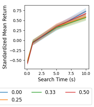
Figure 10 and Figure 11 show the performance of POTMMCP using different values for the hyperparameter.

Appendix E Search depth
Figure 12 shows the maximum search depth by planning time for POTMMCP and baseline planning methods.

Appendix F Evaluation of different meta-policies
Figure 13 shows the performance of POTMMCP using the different meta-policies in each environment.

Appendix G Evaluation of different search policies


Appendix H Belief Accuracy
Figure 16 shows POTMMCP’s belief accuracy for each environment.

Appendix I Sensitivity to Novel Policies
These results were not included in the main paper since they were outside the assumptions of our method. However, we include them here for reference and to motivate future research.
Figure 17 show the performance of POTMMCP and baselines when paired with other agents using policies from that are not included in the set of known policies . The policies in were generated in the same way as those within the set , but with a different seed leading to differences in behaviours. From the results we can see that POTMMCP is more robust to the out-of-distribution policies than the I-POMCP-PF baselines, and shown by the higher mean return. However, POTMMCP’s performance against the new policies is significantly lower when compared to its performance against the known policies (Figure 3), suggesting that POTMMCP is sensitive to out-of-distribution policies at least for the policy prior used in our experiments. This presents an interesting follow-up question. Specifically, what types of policy priors can lead to more robust performance?
