Lattice calculation of the meson radiative form factors over the full kinematical range
Abstract
We compute the structure-dependent axial and vector form factors for the radiative leptonic decays , where is a charged lepton, as functions of the energy of the photon in the rest frame of the meson. The computation is performed using gauge-field configurations with 2+1+1 sea-quark flavours generated by the European Twisted Mass Collaboration and the results have been extrapolated to the continuum limit. For the vector form factor we observe a very significant partial cancellation between the contributions from the emission of the photon from the strange quark and that from the charm quark. The results for the form factors are used to test the reliability of various Anzätze based on single-pole dominance and its extensions, and we present a simple parametrization of the form factors which fits our data very well and which can be used in future phenomenological analyses. Using the form factors we compute the differential decay rate and the branching ratio for the process as a function of the lower cut-off on the photon energy. With a cut-off of 10 MeV for example, we find a branching ratio of Br which, unlike some model calculations, is consistent with the upper bound from the BESIII experiment Br at 90% confidence level. Even for photon energies as low as 10 MeV, the decay is dominated by the structure-dependent contribution to the amplitude (unlike the decays with or ), confirming its value in searches for hypothetical new physics as well as in determining the Cabibbo-Kobayashi-Maskawa (CKM) parameters at , where is the fine-structure constant.
I Introduction
The comparison between experimental measurements and theoretical predictions for flavour changing processes accompanied by photon emission represents an important tool in the search of New Physics (NP) beyond the Standard Model (SM). In this paper we consider radiative weak leptonic decays of the form , where is a pseudoscalar meson, a lepton-neutrino pair, and a real photon.
For each meson , in addition to the leptonic decay constant , the computation of the corresponding decay rate requires the calculation of two Structure-Dependent (SD) hadronic form factors, and , which depend on the energy of the photon in the meson rest frame.
If instead the structure dependence of the meson is neglected, i.e. in the “point-like” approximation, the only non-perturbative input required to determine the decay rate is .
An interesting feature of these decays is that, because of helicity suppression, the point-like contribution to the decay rate is suppressed with respect to the SD contribution by the square of the ratio , where and are the masses of the charged lepton and meson respectively.
For heavy mesons and light final-state charged leptons , the SD contribution, which is sensitive to the internal structure of the decaying meson, can already be dominant at relatively low photon energies, and in particular those well below the typical energy cut-off imposed in experimental measurements.
This makes such decay channels an ideal place to probe the internal structure of the meson and the presence of possible NP contributions.
While for pion and kaon decays several experimental measurements of the axial and vector form factors exist (see e.g. Ref. Bychkov:2008ws; E787:2000ehx; KLOE:2009urs; OKA:2019gav; ISTRA:2010smy; JPARCE36:2021yvz), for heavy mesons only very little is known. For charmed meson decays the BESIII collaboration recently searched for signals of the Cabibbo-suppressed decay BESIII:2017whk and of the Cabibbo-favoured one BESIII:2019pjk, finding no events with emission of photons with energies , and setting the following upper bounds on the branching ratios: and at 90% confidence level.
For the meson, the Belle collaboration has recently set the bounds Belle:2015mpp; Belle:2018jqd and , and observed photons with energies . We believe that by providing accurate predictions from first principles for the axial and vector form factors for heavy mesons, we will motivate further experimental studies.
We have recently computed the rates for decays where is a light meson, or , Desiderio:2020oej and compared our results to experimental measurements finding some puzzling and interesting discrepancies yet to be resolved Frezzotti:2020bfa. In Ref. Desiderio:2020oej we have also computed the amplitude for the decays of the meson, but only over part of the physical phase space; specifically for photon energies up to , as measured in the rest frame of the meson.
In this paper, we return to the radiative decays of mesons and compute the relevant axial and vector form factors and over the full physical kinematic range and with high statistical accuracy, thus improving significantly upon the previous study of Ref. Desiderio:2020oej.
The computation is performed using the Wilson-clover twisted-mass gauge ensembles generated by the Extended Twisted Mass Collaboration (ETMC) with quark masses tuned very close to their physical values, for almost all the ensembles Alexandrou:2018egz; ExtendedTwistedMass:2021qui; ExtendedTwistedMass:2021gbo; Alexandrou:2022amy. The ensembles correspond to four values of the lattice spacing in the range , with the spatial extent of the lattice, , ranging from to .
Our main results for the radiative form factors and are collected in Tab. 5 and plotted in Fig. 8, and we provide their correlation matrices in Appendix B.
Recently, numerical results for the lattice computation of and of the meson also have been published in Ref. Giusti:2023pot. The primary focus of that paper however, is on developing and testing different strategies for the lattice computation of the form factors. Their numerical results are based on a single gauge ensemble at an unphysical pion mass, and for this reason a direct comparison with our results is not possible at present. In the future, it would be interesting to compare our results with those obtained from other lattice regularizations in the continuum limit.
We use our results for the form factors to compute the branching fraction of the decay, as a function of the lower cut-off, , on the photon energy, as measured in the meson rest frame. Our results are showed in Fig. 10. For GeV, our prediction for the branching fraction lies well below the experimental upper limit set by the BESIII collaboration BESIII:2019pjk. Due to the strong helicity suppression, the branching fraction is dominated by the SD contribution, even for a lower cut on the photon energy as small as GeV.
In Fig. 11, we show the SD contribution to the differential decay rate, as a function of the photon energy in the meson rest frame; this goes to zero at the edge of phase space and reaches a maximum in the region kinematic .
Having calculated the form factors from first principles in a lattice computation, we test how well model calculations based on single-pole dominance and light-cone sum rules (LCSR) reproduce our results. Such a test is important because model calculations are commonly used to describe the form factors of heavy mesons, in particular the meson Korchemsky:1999qb; Atwood:1994za; Yang:2012jp, for which a direct lattice calculation is currently missing.
We fit our results for the vector and axial form factors of the meson to several pole-like Ansätze, finding that, in general, a pure vector-meson-dominance (VMD) Ansatz does not describe very well the momentum dependence of the data, particularly for the axial form factor . However, by including the leading non-singular corrections in the Laurent expansion around the pole, we obtain a very good description of our lattice data. The resulting fit parameters are collected in Tab. 6 and can be used for future phenomenological analyses.
From the pole-like fits to we extract the coupling , which is the form factor describing the decay. Our estimate of is in good agreement with the direct lattice determination of Ref. Donald:2014 but strongly disagrees with the value predicted by light-cone sum rules (LCSR) at next-to-leading order (NLO) Pullin:2021ebn, from which it differs by a factor 5. LCSR at NLO order were also used to estimate the radiative form factors and of the meson, at one specific kinematical point Lyon:2012fk.
Their estimates disagree very significantly with those from our direct lattice computation, differing by a factor for the vector form factor , and by an order of magnitude and a relative minus sign, for the axial form factor . We conclude that caution should be exercised when using such calculations based on LCSR to predict the heavy-meson radiative form factors. A similar message is conveyed in a recent paper on the decay Guadagnoli:2023zym.
The plan for the remainder of this paper is as follows. In Sec. II we explain how the two structure dependent form factors contributing to the amplitude for decays, and , can be determined from suitable Euclidean lattice correlation functions. In Sec. III we briefly describe the mixed-action lattice framework which we use and present detailed information on the technical aspects of the simulations. Sec. IV contains the determination of the form factors, together with our estimates of the systematic errors, including a description of the extrapolations to the continuum and infinite volume limits. In this section we also present the determination of the differential decay rate and branching fraction, as a function of , for the decay. In Sec. V we provide a simple pole-like parameterization of our data for and , which may be useful for those interested in using our data for phenomenological analyses. We also compare the results presented in Sec. IV with predictions from models based on pole dominance or light-cone sum-rules. Finally in Sec. VI we present our conclusions. There are three appendices to supplement the information in the main text. In Appendix A we explain the reason for the observed deterioration of the signal-to-noise ratio at large photon energies. The results for the form factors and , together with the corresponding correlation matrices are tabulated in Appendix B so that they can be used in phenomenological studies. In Appendix C we present a detailed analysis of single-pole parametrizations of our results for the form factors.
II Definition of the form factors
In order to make this paper self contained, in this section we briefly summarise our conventions and notation, and in particular recall the definition of the structure-dependent form factors which had previously been introduced in Refs. Carrasco:2015xwa; Bijnens:1992en; Desiderio:2020oej; Gagliardi:2022szw. The non-perturbative contribution to the radiative leptonic decay rate for the processes is encoded in the hadronic matrix-element
| (1) |
where implies time-ordering of the two currents, is the polarisation vector of the outgoing photon with four-momentum , is the three-momentum of the meson, and and are the weak and electromagnetic hadronic currents respectively:
| (2) |
where is the electric charge of the flavour . The hadronic tensor can be decomposed in terms of a “point-like” contribution (i.e. the expression obtained by treating the meson as a point-like particle) and four structure-dependent (SD) scalar form factors, and Carrasco:2015xwa; Bijnens:1992en; Desiderio:2020oej; Gagliardi:2022szw 11 1 Here, we use the dimensionless definitions of introduced in Ref. Gagliardi:2022szw which differ by simple factors from those used in our earlier papers Carrasco:2015xwa; Desiderio:2020oej. As explained below, the form factors do not contribute to the decays studied here, i.e. those with a real photon in the final state.:
| (3) | |||||
| (4) | |||||
| (5) |
where is the mass of the meson and its four momentum, with . The point-like contribution saturates the Ward-Identity (WI) satisfied by :
| (6) |
which implies that . Moreover, when integrating over the full three-body phase space, it is only the square of the point-like term which is infrared divergent. At order , this infrared divergence is cancelled by the virtual photon correction to the purely leptonic decay.
Eq. (5) is valid for generic (off-shell) values of the photon four-momentum and can also be used to study the four-body decay , where the are charged leptons, or more generally the decays of any pseudoscalar meson , as we showed in an exploratory work with Gagliardi:2022szw. In this paper we study the emission of a real photon, so that and , and therefore only the axial form factor and the vector form factor , together with the point-like term, contribute to the decay rate for the process .
In the following, as in our previous study Desiderio:2020oej, we find it convenient to evaluate the form factors and as functions of the dimensionless variable
| (7) |
where is the mass of the charged lepton . In the rest frame of the meson ( ) where is the energy of the photon. The above discussion applies to other pseudoscalar mesons (, , , ) with the natural replacement of in Eqs. (1) - (7) by the meson being studied and the corresponding change of the quark flavours in the weak current in Eq. (2).
II.1 Evaluating and from Euclidean lattice correlation functions
In Sec. III and Appendix B of Ref. Desiderio:2020oej we showed in detail that for the emission of a real photon, the hadronic tensor can be extracted for all values of from the Euclidean three-point correlation function:
| (8) |
where is the temporal extent of the lattice 22 2 is not to be confused with which represents ”time-ordered”., is an interpolating operator with the quantum numbers to create the meson, , and is the energy of the photon. In the forward half of the lattice for example, one has
| (9) |
where the ellipsis indicates terms that vanish exponentially in the large limit and . Eq. (8) is valid for , however, as explained in Appendix B of Ref. Desiderio:2020oej, can be obtained also from the backward half of the lattice exploiting time-reversal symmetry. In order to determine the form factors and it is convenient to distinguish the contributions from the vector and axial-vector components of the weak current, , and to write
| (10) |


The Wick contractions of the correlation function in Eq. (8) give rise to two distinct topologies of Feynman diagrams, namely to quark-line connected and quark-line disconnected diagrams; these are illustrated in Fig. 1. In the disconnected diagrams the photon is emitted from a sea quark. This contribution vanishes in the -symmetric limit and is neglected in the present study; this is the so-called electroquenched approximation. We focus instead on the calculation of the dominant, quark-connected contributions for which as explained in Ref. Desiderio:2020oej, it is possible to use twisted boundary conditions to assign arbitrary values to momenta of the photon and -meson, and respectively, at the price of violations of unitarity which vanish exponentially with the lattice extent Sachrajda:2004mi; Flynn:2007ess. This is achieved by treating the two quark propagators related to the electromagnetic current in the right-hand diagram of Fig. 1 as corresponding to two distinct quark fields having the same mass and quantum number, but satisfying different spatial boundary conditions. Defining to be the spectator quark-field in the right-hand diagram of Fig. 1, we set the spatial boundary conditions of the three quark fields as follows:
| (11) |
where are arbitrary spatial-vectors of angles, in terms of which the photon and meson lattice momenta are given by
| (12) |
where is the lattice spacing. The results presented in the following sections have been obtained in the rest frame of the meson () and with the photon momentum chosen to be in the -direction, , i.e. by setting
| (13) |
With such a choice of kinematics, the two form factors and can be obtained from the large-time behaviour, , of the following two estimators
| (14) | ||||
| (15) |
where and, since for a real photon is determined by , we have redefined
| (16) |
where we used the lattice dispersion relation for the photon energy. Notice that in the estimator of the axial form factor, the zero-momentum subtraction serves to remove the point-like contribution proportional to . As discussed in Sec. IV of Ref. Desiderio:2020oej, the subtractions in Eq. (15) of and at allow us to isolate the SD form factor without generating infrared-divergent cut-off effects of order . Such dangerous discretization effects, which could hinder the determination of at small values of , are present instead if one subtracts the point-like contribution in Eq. (1), using the value of the decay constant determined from two-point correlation functions.
III Details of the computation
Our results have been obtained using the gauge field configurations generated by the Extended Twisted Mass Collaboration (ETMC) employing the Iwasaki gluon action Iwasaki:1985we and flavours of Wilson-Clover twisted-mass fermions at maximal twist Frezzotti:2000nk. This framework guarantees the automatic improvement of parity-even observables Frezzotti:2003ni; Frezzotti:2004wz. A detailed description of the ETMC ensembles can be found in Refs. ExtendedTwistedMass:2021gbo; ExtendedTwistedMass:2021qui; Alexandrou:2022amy; Alexandrou:2018egz, while essential informations on the ensembles we have used in the present work are collected in Table 1. The ensembles listed in Table 1 correspond to four values of the lattice spacing in the range , and lattice extent in the range . The mass of the light sea quarks on the three finest ensembles, has been tuned so as to give almost physical-mass pions, while on the coarsest ensemble the pion mass33 3 For the present study of the meson, the presence of a heavier-than-physical pion, with mass , on the coarsest ensemble does not require a chiral extrapolation since we expect that the form factors are largely insensitive to the value of the masses of the light sea quarks. is . For all the ensembles, the strange and charm sea-quark masses are set to within about 5% of their physical values, defined through the requirement that (see Refs. Alexandrou:2018egz; ExtendedTwistedMass:2021qui; Alexandrou:2022amy for more details)
| (17) |
| ensemble | (fm) | (MeV) | (fm) | ||||
|---|---|---|---|---|---|---|---|
| cA211.12.48 | |||||||
| cB211.072.64 | |||||||
| cC211.060.80 | |||||||
| cD211.054.96 |
We work in a mixed-action framework in which the valence strange and charm quarks are discretized as Osterwalder-Seiler fermions Osterwalder:1977pc; Frezzotti:2004wz. The corresponding valence bare-quark mass parameters and , have been tuned to reproduce the value of the pseudoscalar mass 44 4 The is a fictitious pseudoscalar meson made of two different mass-degenerate quarks and having mass equal to that of the strange quark. Its mass is equivalent to that of the meson if one neglects quark-line disconnected contributions. determined in Ref. Borsanyi:2020mff and the PDG value ParticleDataGroup:2020ssz of the pseudoscalar mass (see Appendix C of Ref. Alexandrou:2022amy for more details)
| (18) |
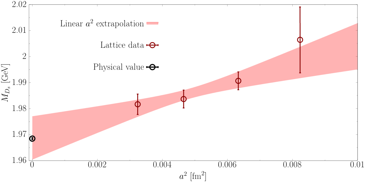
where the error in includes, in addition to the experimental uncertainty, an estimate of the contribution from the neglected disconnected diagrams Hatton:2020qhk; Zhang:2021xrs. The values of and used for each of the ensembles of Table 1 are collected in Table 2. Since the strange and charm quark masses have been fixed using the mass of the and mesons, the mass of the meson deviates from the physical value by cut-off effects, as we show in Figure 2.
On each ensemble, we have analyzed gauge configurations and performed the inversions of the Dirac operator on 4 stochastic sources. The sources are randomly distributed over time, diagonal in spin and dense in the color. The interpolating operator has been smeared as in our previous works using Gaussian smearing (see e.g. Ref. Carrasco:2014uya for more details). We employ a local discretization of the weak current:
| (19) |
Note that at maximal-twist the Renormalization Constants (RCs) to be used for and are chirally-rotated w.r.t. the ones of standard Wilson-fermions, and the bare vector () and axial-vector () currents renormalize respectively with multiplicative renormalization constants and .
| Ensemble | ||
|---|---|---|
| cA211.12.48 | 0.0200 | 0.2725 |
| cB211.072.64 | 0.0184 | 0.2370 |
| cC211.060.80 | 0.0162 | 0.2019 |
| cD211.054.96 | 0.0136 | 0.1671 |
For the electromagnetic current , we use the exactly-conserved point-split current
| (20) |
where are the QCD gauge links, and is the sign of the chirally-rotated Wilson term used for flavour . In the electroquenched approximation only the and terms in contribute to the correlation function in Eq. (8). In our numerical simulations, we have chosen opposite signs for the chirally-rotated twisted term of the strange and charm valence quarks, . We evaluate the correlation functions in Eq. (8) and the estimators in Eq. (9) using the bare currents in Eq. (19) and the point split electromagnetic current in Eq. (20).
The RC which renormalizes the current , is determined from the large-time behaviour of the following estimator
| (21) |
In the twisted-mass framework which we are using, the decay constant can be determined from the large-time behaviour of the two-point correlation function , without the need of additional renormalization, using
| (22) |
and
| (23) |
where the strange and charm quark fields entering in Eq. (22) carry opposite signs of the chirally-rotated twisted term. In practice, we find it convenient to define the following estimators to extract the physical form factors and
| (24) |
where the values of the ratio used for each of the ensembles in Table 1, are taken from the analysis of Ref. Alexandrou:2022amy, and reported in Table 3.
| ensemble | |
|---|---|
| cA211.12.48 | |
| cB211.072.64 | |
| cC211.060.80 | |
| cD211.054.96 |
IV Numerical results
In this section we present the numerical results for the form factors and at ten evenly spaced values of (Subsec IV.1). We then use these results to calculate the differential decay rate and branching fraction for the process (Subsec IV.2).
IV.1 Results for the form factors
In order to determine the form factors, we evaluate the estimators at ten evenly-spaced values of the dimensionless variable :
| (25) |
At finite lattice spacing , the relations between the twist angle , the photon momentum and are obtained from Eqs. (12) and (16):
| (26) |
For each gauge ensemble, we obtain each of the values of by tuning the twisting angle using the relations in Eq. (26) and the value of . The resulting statistical uncertainty on the values of is negligibly small (typically below ). For an illustration of the quality of the plateaus, we present in Figs. 3 and 4 the estimators for selected values of , obtained on the ensembles cB211.072.64 (B64 for short) and cC211.06.80 (C80 for short) respectively. In each figure the blue band shows the values of obtained from a constant fit in the region where the estimators display a plateau 55 5 We have checked that the results are stable under small shifts, in both forward and backward direction, of the time intervals adopted in the constant fit..


As is clear from the figures, we observe a rapid deterioration of the signal for both and at large values of . In particular the statistical errors on turn out to be very large at small values of , and then progressively decrease as increases. The origin of this peculiar behaviour, which is discussed in detail in Appendix A, is due to the existence of a threshold value of above which the intrinsic statistical fluctuations of start to grow asymptotically with . As argued in Appendix A, this threshold value of is given by the mass of the lightest pseudoscalar meson state with . The outcome of the analysis is that for , the fluctuation of scales asymptotically as
| (27) |
where is a prefactor and the ellipsis indicate terms that are subleading in the limit . For the meson (see footnote 4 for the definition of ) so that the threshold value of at which the error on starts to grow asymptotically is given by , in agreement with our numerical results. Notice that in Eq. (27) is finite only because of the finite temporal extent of the lattice, and the signal-to-noise (S/N) problem is thus amplified on large lattices. In addition, the S/N problem becomes much more severe for heavy-light mesons with a or valence quark,
such as or mesons, where is proportional to the ratio between the pion mass and . Large errors are therefore to be expected even for rather small values of . A way forward to mitigate this problem is briefly discussed at the end of Appendix A. We note that the approach that we propose in Appendix.A to tame the S/N problem in Eq. (27) has been discussed in great detail in Ref. Giusti:2023pot where it was called the method. In Ref. Giusti:2023pot the authors provide a detailed comparison, on a single coarse ensemble with , , and , of the unwanted exponential contamination appearing in the method and in the approach we use in the present work, based on the study of the three-point correlation function in Eq. (8) (in Ref. Giusti:2023pot this approach goes by the name of the method). On the single ensemble analyzed, the authors of Ref. Giusti:2023pot find that the method gives a better control over the unwanted exponentials. Here, we argue that the method can also be helpful to tame the exponential problem for .
The ensembles of Table 1 all correspond to lattices with a spatial extent in the range - . While these volumes are expected to be large enough for the finite-size effects (FSEs) on and to be small, in order to estimate the residual FSEs, we have also used a fifth ensemble, the cB211.072.96 ensemble (B96 for short), with the same parameters as the B64 ensemble, except that is a factor larger. We have measured both and on the B96 ensemble up to using gauge configurations 66 6 Beyond the statistical errors on the B96 ensemble are too big for the results to be useful. Indeed, since on the B96 ensemble , the exponential increase of the error with the photon energy described by Eq. (27), is much faster than the one present on the B64 ensemble.. As a conservative estimate of the FSEs, we associate to the values of determined on each of the ensembles of Table 1 an additional systematic uncertainty given by 77 7 For we associate the same relative systematic uncertainty as determined for .
| (28) |
where the subscript represents or and
| (29) |
which is the relative spread between the results obtained on the B96 and B64 ensembles, weighted by the probability that the spread is not due to a statistical fluctuation. In Fig. (5) we compare the two estimators and , at two selected kinematic points and , determined on the B64 and B96 ensembles.


Reassuringly, we find that for all values of and for both form factors is smaller or of a similar size than the corresponding statistical uncertainty, and the difference between the results on the two volumes are most probably largely due to statistical fluctuations.
Next we consider cut-off effects. For each value of the extrapolation to the continuum limit is performed using the following Ansatz
| (30) |
with the parameter chosen to be 88 8 With such a choice we find that the are of (see Table 4 below). and and are dimensionless fit parameters which depend on and are different for the two channels . The result of the extrapolation for and , obtained using the Ansatz in Eq. (30) with the fit parameter fixed to zero, are shown in Figs. 6 and 7.


In the two figures, the blue bands correspond to the linear extrapolation, performed omitting the measurement at the coarsest value of the lattice spacing. In Table 4, we report the values of the parameters obtained from the linear -fit to the full dataset (orange band in Figs 6 and 7) , along with the corresponding reduced , which is always very good, except for at the largest two values of ( and ).
| d.o.f. | d.o.f. | |||||
|---|---|---|---|---|---|---|
| 0.1 | -0.189 | 0.063 | 0.070 | -0.197 | 0.132 | 0.656 |
| 0.2 | -0.262 | 0.057 | 0.105 | -0.339 | 0.038 | 0.786 |
| 0.3 | -0.325 | 0.049 | 0.147 | -0.414 | 0.024 | 0.396 |
| 0.4 | -0.382 | 0.045 | 0.123 | -0.470 | 0.019 | 0.089 |
| 0.5 | -0.430 | 0.040 | 0.179 | -0.517 | 0.017 | 0.488 |
| 0.6 | -0.480 | 0.041 | 0.158 | -0.551 | 0.016 | 1.597 |
| 0.7 | -0.531 | 0.041 | 0.174 | -0.595 | 0.018 | 0.946 |
| 0.8 | -0.594 | 0.055 | 0.750 | -0.676 | 0.030 | 0.510 |
| 0.9 | -0.726 | 0.079 | 1.927 | -0.824 | 0.063 | 0.756 |
| 1.0 | -0.940 | 0.122 | 2.023 | -0.964 | 0.123 | 0.241 |
For most values of , the fit parameter turns out to be of order , suggesting the presence of cut-off effects in and that are of order .
We find that including the terms leads to overfitting without substantially improving the quality of the fit. The continuum values obtained using the Ansatz of Eq. (30) are always consistent within errors with those obtained from linear fits (i.e. with set to 0) shown in Figs. 6 and 7, but have substantially larger statistical uncertainties. Moreover, the coefficient turns out to be always consistent with zero within - standard deviations, a clear signal of overfitting. Given these observations we have decided to estimate the systematic uncertainty due to the continuum extrapolation, using the two linear extrapolations shown in each of Figs. 6 and 7. Let and represent generically the continuum values of or at some value of obtained respectively from the linear fit by including or omitting the result at the coarsest lattice spacing. We determine the final central value through a weighted average of the form
| (31) |
Our estimate of the systematic error, which is added in quadrature to the combined statistical and finite-volume uncertainty, is then obtained using
| (32) |
The weights , with , are chosen according to the Akaike Information Criterion Akaike (AIC) proposed in Ref. Neil:2022joj, namely
| (33) |
where is the total obtained in the -th fit, and and are the corresponding number of fit parameters and measurements99
9
We have checked that the use of uniform weights, , leads to very similar results..
In Fig. 8 we show our final determination of the axial and vector form factors as a function of .


The error bars include all the systematic uncertainties discussed above. The results for and are compared with those of Ref. Desiderio:2020oej, in which only the phase space region up to had been explored. As the figures show, our results are in good agreement with those of Ref. Desiderio:2020oej for both and , while the statistical uncertainty of the results is significantly improved, particularly for . In Table 5 we collect our final results for the continuum values of and , while in Appendix B we present the full correlation matrix between the form factors evaluated at different values of , which may be useful for phenomenological analyses.
0.1 0.0813 0.0054 -0.1048 0.0097 0.2 0.0715 0.0041 -0.0819 0.0028 0.3 0.0641 0.0033 -0.0643 0.0013 0.4 0.0582 0.0028 -0.0519 0.0008 0.5 0.0534 0.0021 -0.0431 0.0008 0.6 0.0495 0.0024 -0.0363 0.0008 0.7 0.0463 0.0031 -0.0316 0.0007 0.8 0.0432 0.0032 -0.0291 0.0010 0.9 0.0433 0.0083 -0.0297 0.0056 1.0 0.0489 0.0229 -0.0315 0.0152
We have also determined separately the contributions to the form factors from the emission of the photon from the strange quark or the charm quark. In practice, the strange-quark (charm-quark) contribution to , indicated in the following by (), is obtained by setting the electric charge () in the evaluation of in Eq. (8). The estimators and are obtained using the usual ratio of RCs of Table 3 and the factor of Eq. (21) so that
| (34) |
In Fig. 9 we show the strange- and charm-quark contributions to and , obtained after extrapolating the results to the continuum limit following the same procedure as for the sum.
It is interesting to note that while it is completely dominated by the strange-quark contribution, there is a very significant cancellation between the strange and charm contributions to the vector form factor . The cancellation between the two contributions becomes more pronounced at large values of . The implications of this cancellation in the vector form factor will be discussed in the next section. Finally, as is clear from Fig. 9, at large values of only the errors on increase exponentially, while no degradation of the signal is present for , as expected from the analysis presented in Appendix A.
IV.2 Differential Decay Rate and Branching Fraction
From the knowledge of the SD form factors and , the differential decay rate can readily be evaluated. The relevant formulae have been derived e.g. in Eqs. (1) - (31) of Ref. Frezzotti:2020bfa, to which we refer the reader for a more detailed discussion. However, for the sake of completeness we briefly summarize them here. The differential decay rate is expressed as a sum of three different contributions:
| (35) |
where is the leptonic decay rate in the absence of electromagnetism and is given explicitly by
| (36) |
and the three quantities , , and correspond respectively to the point-like, interference, and SD contribution. The point-like contribution does not depend on the SD form factors, while the interference and the SD contribution depend on and linearly and quadratically, respectively. The explicit expression of the three terms is the following ():
| (37) | |||||
| (38) | |||||
| (39) |
The total decay rate
| (40) |
can be then evaluated for any desired photon energy cut using the previous formulae and our determination of the form factors and . As Eqs. (37) - (39) indicate, the point-like contribution gives rise, in the soft photon limit , to a logarithmically divergent contribution proportional to and is therefore the dominant contribution in for sufficiently small values of 1010 10 The infrared divergence in the leptonic decay with a real photon in the final state is cancelled by the virtual photon contribution to the purely leptonic decay amplitude, through the Bloch-Nordsieck mechanism PhysRev.52.54. The inclusive leptonic decay rate is infrared finite.. However, the pointlike contribution is also chirally suppressed with respect to the SD contribution by the factor . Unlike the point-like contribution, the SD contribution to is small at small photon energies, then grows reaching a maximum at some value of the photon energy which depends on the specific channel considered, and then decreases to zero at the edge of phase space, i.e. for . Therefore, for a sufficiently large photon energy cut-off and a small value of , the SD contribution to is the dominant one.
For the radiative leptonic decays of the meson, the only experimental measurement that is currently available is the branching fraction for , for which the BESIII collaboration has given the upper bound at 90% confidence level BESIII:2019pjk
| (41) |
including photons with energies . Because of the small mass of the electron, compared to and , the electron channel is the most sensitive to the vector and axial form factors and and is therefore the most interesting one phenomenologically. In Fig. 10 we show our determination of the branching fraction as a function of the cut-off on the photon energy, starting from the cut employed by the BESIII collaboration in Ref. BESIII:2019pjk, which is indicated in the figure by the dashed red line.

For this calculation, we used the following values of the CKM matrix element and of the decay constant, which we have taken from the 2021 FLAG review FlavourLatticeAveragingGroupFLAG:2021npn
| (42) |
We have computed the branching fraction by using the form factors determined either from the spline interpolation of our numerical lattice results or by fitting to the phenomenological parametrization of the form factors given in Eq. (43) below and discussed in the next section.
The two different determinations of the branching fraction are represented in Fig. 10 by the blue and red bands respectively.
The phenomenological parametrization of the form factor leads to a much more precise determination of the form factors in the kinematical region of high values of than the spline interpolation of the lattice data. This is due to the fact that the fit parameters are mainly determined from the most statistically accurate data points, which are the ones at low and intermediate values of , while the spline interpolation is designed to always reproduce the actual data points with their corresponding error range. As a consequence, the branching fraction obtained through the phenomenological parametrization of the form factors is more precise than the one obtained by using the spline interpolation, and the difference in the precision increases as the lower cut-off on the photon energy increases. On the other hand, results obtained by using the spline interpolation of the lattice data are less affected by potential systematic effects due to model dependence and for this reason we conservatively consider these as our final results. Note however, that the two determinations of the branching fraction are always compatible within errors.
From Fig. 10 we see that the results obtained for using either the spline interpolation () or the phenomenological parametrization of the form factors () are well within the upper bound at 90% confidence level set by the BESIII collaboration (). Moreover, they are also much smaller than the quark-model predictions of Refs. Geng:2000if; Lu:2002mn which estimate a branching fraction of order , and of the determination of Ref. Korchemsky:1999qb where a branching fraction of order is obtained combining perturbative QCD with the heavy-quark effective theory. We find that, already for and even more so for higher-energy cuts, the decay rate is completely dominated by the SD term. The point-like contribution is always below one percent and the interference contribution is even smaller. For comparison, adopting the same cut on the photon energy (), the corresponding branchings into muon or are respectively and , and in both cases are dominated by the point-like contribution. Finally, in Fig. 11 we provide our determination of the SD contribution to the differential branching fraction in the electron channel, which has a maximum for a value of of about . The blue and red bands in Fig. 11 represent respectively the results obtained by using the spline interpolation of the lattice results for the form factors or the phenomenological parametrization based on their fit to the Ansatz of Eq. (43) below. As before, in the region of high values of the results based on the phenomenological parametrization of the form factors become much more precise than the ones based on their spline interpolation. However, the two determinations are always compatible within errors.

Additional branching fractions, with specific cuts on the photon and/or lepton energies, are available on request from the authors.
V Phenomenological parameterization of the form factors
In this section we present a parameterization of the form factors inspired by single-pole dominance. In this approximation the form factor is described in terms of the propagation of the nearest resonance. We find that a good description of the momentum dependence of our lattice data is obtained by employing the following Ansatz:
| (43) |
in which the single-pole dominance approximation corresponds to fixing where is the mass of the nearest resonance, and setting . Here instead , and are three free parameters to be determined from the fit. The constant term represents the leading, non-singular correction in the Laurent expansion of a function around a pole. We refer the reader to Appendix C for a more detailed analysis of the different Ansätze which we have examined.
The Ansatz of Eq. (43) has also been used to fit separately the contributions from the emission of the photon from the charm and strange valence quarks. These are simply obtained by setting the charge of the other quark to zero. We label these separate contributions by and , where the superscript indicates the quark from which the photon has been emitted. Interestingly, we find that including the parameter is only required to obtain an acceptable fit for the separate contributions and . For all the other cases (, , and ), can be set to 0 without increasing the /d.o.f., resulting in good parametrizations of the form factors.
| cor() | cor() | cor() | d.o.f. | ||||
| (fixed) | |||||||
| (fixed) | |||||||
| (fixed) | |||||||
| (fixed) | |||||||


The results of the fits are reported in Tab. 6, while in Fig. 12 we plot the resulting fitting functions together with our lattice data. We see from Fig. 12 and Tab. 6 that the fits provide a very good representation of our lattice data and low values of the correlated , even for the most precisely determined form factors. The remarkably strong, , cancellation between the obtained values of and in Table 6 explains why can be dropped when fitting the total vector form factor. The degree of cancellation between and , and also between the contributions to the form factor from and in the lower panel of Fig. 9, depends on both the charges and masses of the two valence quarks and should therefore be considered to be accidental. It will be interesting in the future to observe to what extent these cancellations hold for the decays of the -meson. Finally, we observe that the parametrization we provide for the form factors is more precise than the lattice data points for kinematics above the threshold value . This is because the fit parameters are mainly determined from the most statistically accurate data points, which are the ones at low and intermediate values of .
Single pole dominance implies that the values of and are related respectively to the masses of the nearest internal resonances contributing to the correlator and to their transition amplitudes to the external states. In the present case, the resonances are the for the vector channel and the for the axial one. The values of the amplitudes are therefore related to the couplings and , i.e. to the and decay amplitudes respectively. However, for such an interpretation of the to be considered to be physically meaningful, we first need to check that the fitted values are stable under variations of the fit Ansatz. We perform such an analysis in detail in Appendix C. The outcome is that the data in the axial channel, i.e. for , and , are well described by any of the different Ansätze we employed, but the resulting values for the amplitude are very different depending on the Ansatz which was used. We conclude that the fitted value of is not stable and is not reliable as an estimate of the coupling . Note that in the axial channel, there is a second resonance, the , with a mass which is only 76 MeV above the nearest resonance, the . Since the difference in the masses is so small, the fitted residue may encode contributions from both of these internal states, resulting in an unreliable determination of the coupling . For the vector channel on the other hand, we found that the value of is very stable under variations of the fit Ansatz, provided that the corresponding fits result in a low value of d.o.f. .
Having established in Appendix C that the value of is stable, we obtain the corresponding value of the coupling , using the relation:
| (44) |
where is the decay constant of the meson, for which we take the value MeV obtained from the lattice computation of Ref. Lubicz:2017. In Tab. 7, we report our estimate for the coupling , and for the individual contributions from the radiation from the strange and charm quarks. In the quoted uncertainties, we include an estimate of the systematic error due to the use of single-pole dominance as a model parameterization of the form factors. This is obtained in Appendix C from the variation of the results in Tab. 9 determined using different Ansätze. In Table 7 we also provide a comparison of our results with the values of the couplings obtained from a direct lattice computation of the decay amplitude Donald:2014, and from the calculation based on LCSR at next-to-leading order Pullin:2021ebn. Our results are in excellent agreement with those of Ref. Donald:2014 and with the value of obtained in the LCSR calculation Pullin:2021ebn. However, we find a discrepancy of a factor of about 2 with the value of obtained in Ref. Pullin:2021ebn which, given the strong cancellation between the strange and charm-quark contributions, is amplified in the total coupling to a factor of about 5; specifically the value from the LCSR calculation is about five times larger than the ones obtained from the lattice computations 1111 11 According to Ref. rzwicky the uncertainty in the coupling given in Ref. Pullin:2021ebn may be an underestimate because of the significant cancellation between the charm and the strange quark contributions.
The authors of Ref. Lyon:2012fk have also provided the values of the radiative form factors and for the meson at a single kinematic point ; and . They add that they refrain from estimating the uncertainties on these values as they ”only aim to provide rough estimates in order to motivate experimental searches” Lyon:2012fk. Nevertheless, these estimates are in strong disagreement with the values collected in Table 5 from our direct lattice computation. In particular, we notice that, around this specific kinematic point, the magnitudes of differ by approximately a factor , while for the results differ by an order of magnitude and have the opposite sign. This raises some questions about the precision of the approach of Refs.Pullin:2021ebn and Lyon:2012fk, based on LCSR, for describing heavy-meson radiative form factors.
| LCSR Pullin:2021ebn | HPQCD Donald:2014 | This paper | |
|---|---|---|---|
VI Conclusions
In this paper we have presented a lattice calculation, in the electro-quenched approximation, of the structure-dependent axial and vector form factors, and , which contribute to the amplitudes for the radiative leptonic decays . Our results extend and improve the analysis presented in Ref. Desiderio:2020oej, and are the first lattice predictions for these form factors over the whole physical phase space in the continuum limit.
We have also presented the individual contributions to the form factors from the emission of the photon from the charm and strange valence quarks, and respectively, with .
A remarkable feature is that , see the lower panel of Fig. 9, so that there is a very significant cancellation in the determination of . The axial form factor is dominated by and
there is no such cancellation, see the upper panel of Fig. 9.
We use our results for the form factors to compute the differential decay rate for the process as a function of the photon energy in the meson rest frame, separating the SD contribution from the point-like one.
By integrating the differential decay rate, we obtain the branching ratio for the decay as a function of the lower cut-off, , on the energy of the photon in the rest frame of the decaying meson. Our result for the branching ratio for MeV is , well
below the upper bound of set by the BESIII collaboration BESIII:2019pjk. Even for as low a value of as 10 MeV, we find that the
the SD contribution dominates the branching ratio due to the strong helicity suppression, by a factor , of the point-like term.
Having determined the form factors, we use the results to investigate the validity and applicability of model-dependent calculations, such as ones based on single-pole dominance or light-cone sum rules.
Such model estimates are commonly used in the analysis of radiative processes involving heavy mesons for which lattice calculations are often not available. We showed that the LCSR computations at next-to-leading order of Refs. Pullin:2021ebn; Lyon:2012fk fail to reproduce our results for the form factors of the meson, and that a pure VMD parametrization does not always reproduce their momentum behavior. In Eq. (43) and Tab. 6 we propose a simple parametrization of the form factors, based on an
extension of the single-pole dominance Ansatz, which reproduces our lattice results very well and may therefore be useful for future phenomenological analyses.
For we find that results for the residue of the pole are very stable, allowing us to interpret the result in terms of the coupling. The result is presented in Tab. 7, where it is also compared to the results from a direct lattice computation of the rate for the decay Donald:2014 (we find good agreement) and to the LCSR calculation of Ref.Pullin:2021ebn (we disagree significantly).
A non-perturbative, model-independent theoretical prediction for the amplitudes of real photon emission in leptonic decays is important for testing the Standard Model and for searches for new physics. Indeed, such results are required in order to include corrections in the determination of fundamental SM parameters such as the CKM matrix elements. In addition, the SD contribution to decays probes the internal structure of the decaying meson and by comparing SM results for the form factors to experimental measurements one can test for hypothetical new physics effects. This is especially true for the decays of heavy mesons into an electron and its neutrino, where the SD contribution dominates the rate already at low photon energies such as 10 MeV, which are included in some current experimental studies. First-principles lattice computations are particularly important for heavy mesons since chiral perturbation theory does not apply in that case. For this reason, in the future we plan to compute the radiative SD form factors also for the and mesons. When applying the strategy that we have presented in this work to these mesons however, the presence of a light valence quark will significantly lower the threshold value of the photon energy above which statistical fluctuation start to grow exponentially. We have identified the origin of this issue in Appendix A, where we also briefly discuss a possible way to mitigate this problem based on the different lattice approach proposed in Ref. Giusti:2023pot, where it is called the method.
VII Acknowledgements
We thank all members of the ETMC for the most enjoyable collaboration. We thank Roman Zwicky for interesting correspondence and discussions and for suggesting that we compute the contributions to the form factors from the emission of the photon from the strange and charm quarks separately. We acknowledge CINECA for the provision of CPU time under the specific initiative INFN-LQCD123 and IscrB_S-EPIC. F.S. G.G and S.S. are supported by the Italian Ministry of University and Research (MIUR) under grant PRIN20172LNEEZ. F.S. and G.G are supported by INFN under GRANT73/CALAT. C.T.S. was partially supported by an Emeritus Fellowship from the Leverhulme Trust and by STFC (UK) grant ST/T000775/1. F.S. is supported by ICSC – Centro Nazionale di Ricerca in High Performance Computing, Big Data and Quantum Computing, funded by European Union – NextGenerationEU.
References
- (1) M. Bychkov et al., New Precise Measurement of the Pion Weak Form Factors in Decay, Phys. Rev. Lett. 103 (2009) 051802 [0804.1815].
- (2) E787 collaboration, Measurement of structure dependent K+ — muon+ neutrino(muon) gamma decay, Phys. Rev. Lett. 85 (2000) 2256 [hep-ex/0003019].
- (3) KLOE collaboration, Precise measurement of and study of , Eur. Phys. J. C 64 (2009) 627 [0907.3594].
- (4) OKA collaboration, Measurement of the decay form factors in the OKA experiment, Eur. Phys. J. C 79 (2019) 635 [1904.10078].
- (5) ISTRA+ collaboration, Extraction of Kaon Formfactors from Decay at ISTRA+ Setup, Phys. Lett. B 695 (2011) 59 [1005.3517].
- (6) J-PARC E36 collaboration, Measurement of structure dependent radiative decays using stopped positive kaons, Phys. Lett. B 826 (2022) 136913 [2107.03583].
- (7) BESIII collaboration, Search for the radiative leptonic decay , Phys. Rev. D 95 (2017) 071102 [1702.05837].
- (8) BESIII collaboration, Search for the decay , Phys. Rev. D 99 (2019) 072002 [1902.03351].
- (9) Belle collaboration, Search for decays with hadronic tagging using the full Belle data sample, Phys. Rev. D 91 (2015) 112009 [1504.05831].
- (10) Belle collaboration, Search for the rare decay of with improved hadronic tagging, Phys. Rev. D 98 (2018) 112016 [1810.12976].
- (11) A. Desiderio et al., First lattice calculation of radiative leptonic decay rates of pseudoscalar mesons, Phys. Rev. D 103 (2021) 014502 [2006.05358].
- (12) R. Frezzotti, M. Garofalo, V. Lubicz, G. Martinelli, C.T. Sachrajda, F. Sanfilippo et al., Comparison of lattice QCD+QED predictions for radiative leptonic decays of light mesons with experimental data, Phys. Rev. D 103 (2021) 053005 [2012.02120].
- (13) C. Alexandrou et al., Simulating twisted mass fermions at physical light, strange and charm quark masses, Phys. Rev. D 98 (2018) 054518 [1807.00495].
- (14) Extended Twisted Mass collaboration, Ratio of kaon and pion leptonic decay constants with Nf=2+1+1 Wilson-clover twisted-mass fermions, Phys. Rev. D 104 (2021) 074520 [2104.06747].
- (15) Extended Twisted Mass collaboration, Quark masses using twisted-mass fermion gauge ensembles, Phys. Rev. D 104 (2021) 074515 [2104.13408].
- (16) C. Alexandrou et al., Lattice calculation of the short and intermediate time-distance hadronic vacuum polarization contributions to the muon magnetic moment using twisted-mass fermions, 2206.15084.
- (17) D. Giusti, C.F. Kane, C. Lehner, S. Meinel and A. Soni, High-precision determination of radiative-leptonic-decay form factors using lattice QCD: a study of methods, 2302.01298.
- (18) G.P. Korchemsky, D. Pirjol and T.-M. Yan, Radiative leptonic decays of B mesons in QCD, Phys. Rev. D 61 (2000) 114510 [hep-ph/9911427].
- (19) D. Atwood, G. Eilam and A. Soni, Pure leptonic radiative decays B+-, D(s) lepton neutrino gamma and the annihilation graph, Mod. Phys. Lett. A 11 (1996) 1061 [hep-ph/9411367].
- (20) J.-C. Yang and M.-Z. Yang, Radiative Leptonic Decays of the charged and Mesons Including Long-Distance Contribution, Mod. Phys. Lett. A 27 (2012) 1250120 [1204.2383].
- (21) HPQCD Collaboration collaboration, Prediction of the width from a calculation of its radiative decay in full lattice qcd, Phys. Rev. Lett. 112 (2014) 212002.
- (22) B. Pullin and R. Zwicky, Radiative decays of heavy-light mesons and the decay constants, JHEP 09 (2021) 023 [2106.13617].
- (23) J. Lyon and R. Zwicky, from Large , Phys. Rev. D 106 (2022) 053001 [1210.6546].
- (24) D. Guadagnoli, C. Normand, S. Simula and L. Vittorio, From in lattice QCD to at high , 2303.02174.
- (25) N. Carrasco, V. Lubicz, G. Martinelli, C.T. Sachrajda, N. Tantalo, C. Tarantino et al., QED Corrections to Hadronic Processes in Lattice QCD, Phys. Rev. D 91 (2015) 074506 [1502.00257].
- (26) J. Bijnens, G. Ecker and J. Gasser, Radiative semileptonic kaon decays, Nucl. Phys. B 396 (1993) 81 [hep-ph/9209261].
- (27) G. Gagliardi, F. Sanfilippo, S. Simula, V. Lubicz, F. Mazzetti, G. Martinelli et al., Virtual photon emission in leptonic decays of charged pseudoscalar mesons, Phys. Rev. D 105 (2022) 114507 [2202.03833].
- (28) C.T. Sachrajda and G. Villadoro, Twisted boundary conditions in lattice simulations, Phys. Lett. B 609 (2005) 73 [hep-lat/0411033].
- (29) J.M. Flynn, A. Juttner, C.T. Sachrajda, P.A. Boyle and J.M. Zanotti, Hadronic form factors in Lattice QCD at small and vanishing momentum transfer, JHEP 05 (2007) 016 [hep-lat/0703005].
- (30) Y. Iwasaki, Renormalization Group Analysis of Lattice Theories and Improved Lattice Action: Two-Dimensional Nonlinear O(N) Sigma Model, Nucl. Phys. B 258 (1985) 141.
- (31) Alpha collaboration, Lattice QCD with a chirally twisted mass term, JHEP 08 (2001) 058 [hep-lat/0101001].
- (32) R. Frezzotti and G.C. Rossi, Chirally improving Wilson fermions. 1. O(a) improvement, JHEP 08 (2004) 007 [hep-lat/0306014].
- (33) R. Frezzotti and G.C. Rossi, Chirally improving Wilson fermions. II. Four-quark operators, JHEP 10 (2004) 070 [hep-lat/0407002].
- (34) Particle Data Group collaboration, Review of Particle Physics, Chin. Phys. C 40 (2016) 100001.
- (35) K. Osterwalder and E. Seiler, Gauge Field Theories on the Lattice, Annals Phys. 110 (1978) 440.
- (36) S. Borsanyi et al., Leading hadronic contribution to the muon magnetic moment from lattice QCD, Nature 593 (2021) 51 [2002.12347].
- (37) Particle Data Group collaboration, Review of Particle Physics, PTEP 2020 (2020) 083C01.
- (38) HPQCD collaboration, Charmonium properties from lattice +QED : Hyperfine splitting, leptonic width, charm quark mass, and , Phys. Rev. D 102 (2020) 054511 [2005.01845].
- (39) R. Zhang, W. Sun, F. Chen, Y. Chen, M. Gong, X. Jiang et al., Annihilation diagram contribution to charmonium masses, Chin. Phys. C 46 (2022) 043102 [2110.01755].
- (40) N. Carrasco et al., mixing in the standard model and beyond from =2 twisted mass QCD, Phys. Rev. D 90 (2014) 014502 [1403.7302].
- (41) H. Akaike, A new look at the statistical model identification, IEEE Transactions on Automatic Control 19 (1974) 716.
- (42) E.T. Neil and J.W. Sitison, Improved information criteria for Bayesian model averaging in lattice field theory, 2208.14983.
- (43) F. Bloch and A. Nordsieck, Note on the radiation field of the electron, Phys. Rev. 52 (1937) 54.
- (44) Flavour Lattice Averaging Group (FLAG) collaboration, FLAG Review 2021, Eur. Phys. J. C 82 (2022) 869 [2111.09849].
- (45) C.Q. Geng, C.C. Lih and W.-M. Zhang, Study of radiative leptonic D meson decays, Mod. Phys. Lett. A 15 (2000) 2087 [hep-ph/0012066].
- (46) C.-D. Lu and G.-L. Song, Radiative leptonic decays of D+-(s) and D+- mesons, Phys. Lett. B 562 (2003) 75 [hep-ph/0212363].
- (47) ETM Collaboration collaboration, Masses and decay constants of and mesons with twisted mass fermions, Phys. Rev. D 96 (2017) 034524.
- (48) R. Zwicky. private communication.
- (49) G. Parisi, The Strategy for Computing the Hadronic Mass Spectrum, Phys. Rept. 103 (1984) 203.
- (50) G.P. Lepage, The Analysis of Algorithms for Lattice Field Theory, in Theoretical Advanced Study Institute in Elementary Particle Physics, 6, 1989.
- (51) Particle Data Group collaboration, Review of Particle Physics, PTEP 2022 (2022) 083C01.
Appendix A Behaviour of the signal-to-noise ratio for and at large
In this appendix, we show why the intrinsic statistical fluctuations of become exponentially large for small values of and large values of . For this discussion we make a certain number of simplifications, but these have no impact on the main conclusions. We consider only the case , i.e. we always work in the decaying hadron’s reference frame. We shall also use continuum notation throughout this appendix, and replace lattice sums by definite integrals. Also, when considering the Euclidean three-point correlation function in Eq. (8) we only consider the term with ,
which is the dominant one in the limit . We discuss the case of an arbitrary pseudoscalar meson made of an up- and a down-type quark.
We choose the 4 momentum and , therefore we now denote the correlation function in Eq. (8) simply by . For it is given by
| (45) |
where
| (46) |
and . We now separate the contribution from the region with from that with :
| (47) | |||||
The time ordering relevant for our discussion is , i.e. with the weak current acting before the electromagnetic current; this corresponds to the second contribution to the correlation function, . We also distinguish the contributions to from the emission of the real photon from the up-type (U) or down-type (D) valence quark, and define
| (48) |
where
| (49) |
in terms of the single flavour contribution to the current,
| (50) |
Since we aim at understanding the behaviour of the error at small , we focus on the case in which the weak current and the interpolating operator are separated by a time distance of a few lattice spacings. In this case, we can interpret the quantity
| (51) |
as a non-local interpolating operator for vector states (in both cases ), and
| (52) |
as a standard two-point correlation function, where vector states propagate between Euclidean time and Euclidean time . Ignoring finite volume interactions, a standard application of the Parisi Parisi:1983ae and Lepage Lepage:1989hd argument, shows that at fixed time and large-time separations , the variance of decreases exponentially as
| (53) |
with the mass of the lightest pseudoscalar state. Instead, the signal scales asymptotically as
| (54) |
where is the mass of the lightest vector state interpolated by . This implies the following asymptotic scaling of the signal-to-noise (S/N) ratio of
| (55) |
Eqs. (53)-(55) enable us to understand the scaling of the error as we discuss in the following subsection. When , we have , , and . We underline that Eqs. (53)-(55) only hold for large time separations .
A.1 Analysis of the scaling of the signal-to-noise ratio of
We now have all the necessary ingredients to understand the scaling of the S/N ratio of . To this end, we define a time, , such that for the asymptotic formulae in Eqs. (53)-(55) hold, i.e. both and are dominated by the contributions from the lowest-energy vector and pseudoscalar intermediate states respectively:
| (56) | ||||
| (57) |
where and for . We thus have 1212 12 In writing Eq. (A.1) we are assuming that the values of at different times are fully correlated, which is a fairly good assumption given that the different times are typically evaluated using the same set of gauge configurations. However, the main result obtained in this appendix, namely the exponential growth of the error in Eq. (60), does not depend upon this assumption.
| (58) | ||||
| (59) |
Since for each value of the photon’s energy, , one has , the integral over in Eq. (58) is always convergent and dominated by the time region where is close to . Indeed, there are no intermediate states lighter than the energy of the external states. However, this is not always the case for the standard deviation . When passing the threshold value the leading exponential contribution in Eq. (A.1) (the term proportional to ) grows asymptotically with and is only regularized by the finite time extent of the lattice. In this case, from the leading exponential term in Eq. (A.1) one has that the divergent part of the error for is given by
| (60) |
The prefactor in Eq. (60) is irrelevant since it does not contribute to (see Eq. (9)) and thus to the hadronic tensor .
The reason behind the behaviour described by Eqs. (58)-(60) is that the kernel function , accounting for the propagation of the photon, weights the different regions in in different ways, giving an exponential enhancement at large times , which are therefore noisier. For real photon emission, the kernel never gives rise to a divergent integral in Eq. (58), since the propagating vector states have non-zero three-momentum so that (see Eq. (54)). However, the states propagating in are at rest, and when , the leading exponential contribution proportional to in Eq. (60) becomes divergent in the limit .
A.2 Numerical checks
For the meson studied in this paper, the threshold value of above which the error starts to grow asymptotically is, according to Eq. (60), given by
| (61) |
For the error will increase only in the contribution to where the photon is emitted from the strange quark, because for the emission from the charm quark, one has , and the corresponding threshold value of is well beyond the physical region explored .
The total error on the strange-quark contribution to (see Eq. (16)) for small times can be modelled as:
| (62) |
where is a background noise term, which we take as being independent from . The contribution to the noise arises from the non-divergent contributions to the noise in Eq. (58) as well as those coming from the first time ordering, , in Eq. (45). Assuming that at the error is large enough such that the term is negligible compared to the one proportional to , we can directly test Eq. (62) against our numerical data. This is shown in Fig. (13) where the error on the strange-quark contribution to is plotted as a function of for two different times . As it is clear from the figure, the data are in remarkably good agreement with the theoretical prediction.
We conclude this appendix with a remark concerning the possibility of extending the calculation of and to the decays of and mesons over the full kinematical range, which is of even greater interest for phenomenology. In light of the above discussion, for these heavy-light mesons the threshold value of the photon energy above which the errors will start to exhibit the exponential behaviour shown in Eq. (60), is given by the pion mass . This means that intrinsically large statistical fluctuations are to be expected in already at very small values of . In this case, a possible step towards avoiding the S/N problem, consists in evaluating the integral over in Eq. (45) on a reduced time interval , and then checking for convergence of the result as a function of . In this way one can expect to avoid including in the integration large values of which do not contribute substantially to the signal (which is dominated by the region of times close to ) but which are responsible for the exponential increase of the error.
However, such approach requires the computation of the Euclidean three points function
| (63) |
for different values of and for all values . In this way it is later possible to perform the integral over for each value of . Computations at several values of need to be performed in order to verify that the ground state has been isolated. This makes the approach more expensive than computing in Eq. (8) directly, which can be done for all values of at the cost of a single sequential propagator. Whether such an extra cost for heavy-light mesons is offset by a significant improvement in accuracy remains to be seen. We plan to investigate this in the future.
Appendix B Results and correlation matrices for and .
Appendix C Analysis of single-pole parameterizations for and
Single-pole dominance, sometimes called Vector Meson Dominance (VMD) in the literature, is a model used to describe the momentum behavior of form factors, as determined by the propagation of the nearest internal resonance contributing to the amplitude. In this appendix we fit the data from our non-perturbative lattice computation of and , to check the validity of such a parameterization. After demonstrating that a pure VMD Ansatz is not consistent with our results for the form factors, we propose a simple extension of the parameterization that can fit our data with good precision over the whole kinematical range. This parameterization provides a simple and practical description of our data which can be used in future phenomenological analyses. We also check the stability of the fitted values of the residues of the singular pole terms in the parameterization (i.e. the in Eq.(43)). This is a necessary test in order to assess the validity of relating the fitted to the and decay amplitudes for the vector and axial channels respectively, as predicted by single-pole dominance.
VMD predictions are obtained by inserting a sum over intermediate states between the two operators in the correlation function defining in Eq. (1) and approximating this sum by the contribution from the nearest state. This approximation is also appropriately called single-pole dominance. For the vector and axial components of the weak current the nearest internal states are the and mesons respectively, contributing to the time-ordering in which the electromagnetic current acts on the initial meson at an earlier time than that at which the weak current is inserted, i.e. in Eq. (8). Thus, by assuming single-pole dominance, we obtain the following parameterization for the momentum behaviour of the form factors 1313 13 Here and in the following, we employ the reference frame in which the initial meson is at rest.:
| (108) | |||||
| (109) |
where and are the masses of the and mesons respectively and and are constant coefficients with the dimension of energy squared. By dividing both the numerator and denominator of Eqs. (108) and (109) by and expressing in terms of as , we obtain
| (110) | |||||
| (111) |
where and are now dimensionless parameters.


By inserting the values MeV, MeV and MeV, taken from the PDG Workman:2022ynf, we obtain the ratios and . Thus, Eqs. (110) and (111) describe the momentum dependence, as predicted by VMD, for the axial and vector form factors, and also for the contributions corresponding to the emission of the photon from the charm and strange quarks separately. In order to check the validity of the VMD prediction, we fit our lattice results to the parameterization of Eqs. (110) and (111), with and taken as free parameters to be determined from the fit1414 14 All the fits of this analysis have been performed by minimizing the correlated .. The results of these fits are shown in the plots in Fig. 14. It is clear from the figure, and confirmed by the corresponding high values of d.o.f., that the results of the fit are in general very poor. The only exception is the VMD fit for the total vector form factor , which proves to be a good fit of our data.
Since the pure VMD fit, with only one free parameter, fails to describe our lattice results for the form factors, we now introduce a more general Ansatz; one that represents the Laurent expansion of a function around a pole:
| (112) |
where we have included corrections up to linear terms in , with , , and being free parameters to be determined from the fit. In Eq. (112), the difference of the parameters from the VMD values and , partially accounts for the contributions from heavier internal states. The free parameters and , that describe the first two non-singular terms of the Laurent expansion of a function around a pole, are also expected to encode non-negligible contributions that are not included in the pure VMD description.
| fitted parameters | |||||
| d.o.f. | |||||
| fit | (fixed) | (fixed) | |||
| fit | (fixed) | ||||
| fit | (fixed) | (fixed | |||
| fit | (fixed) | ||||
| fitted parameters | |||||
| d.o.f. | |||||
| fit | (fixed) | (fixed) | |||
| fit | (fixed) | ||||
| fit | (fixed) | (fixed) | |||
| fit | (fixed) | ||||
| fitted parameters | |||||
| d.o.f. | |||||
| fit | (fixed) | (fixed) | |||
| fit | (fixed) | ||||
| fit | (fixed) | (fixed) | |||
| fit | (fixed) | ||||
| fitted parameters | |||||
| d.o.f. | |||||
| fit | (fixed) | (fixed) | |||
| fit | (fixed) | ||||
| fit | (fixed) | (fixed) | |||
| fit | (fixed) | ||||
| fitted parameters | |||||
| d.o.f. | |||||
| fit | (fixed) | (fixed) | |||
| fit | (fixed) | ||||
| fit | (fixed) | (fixed) | |||
| fit | (fixed) | ||||
| fitted parameters | |||||
| d.o.f. | |||||
| fit | (fixed) | (fixed) | |||
| fit | (fixed) | ||||
| fit | (fixed) | (fixed) | |||
| fit | (fixed) | ||||
| fit | fit | fit | fit | |
|---|---|---|---|---|
In order to check for the stability of the residues and , and hence their interpretation in terms of the and decay amplitudes, we have performed several fits of our data, based on the Ansatz of Eq. (112), fixing on each occasion some of its parameters to their VMD values 1515 15 With the limited number of points for which we have results, it is not possible to perform fits with all four parameters left free to be determined by the fits as this results in overfitting.. Specifically, the fit is performed by fixing , while the fit is performed by setting only . The fit is obtained by fixing and for the vector channel and for the axial one. Finally the fit, obtained by setting for the vector channel and for the axial one, with the remaining 3 parameters determined by the fits. The results of these fits, for each form factor and for their individual charm and strange contributions, are reported in Tab. 8.
From the table, we see that all the different Ansätze provide an adequate fit to our data for the axial channel, but we notice that the fitted values for the residue of the singular term, , obtained from the fit are very different from those obtained from the fits with as a free parameter. Although all three fits with as a free parameter give consistent results for , we avoid relating these results to the decay amplitude for two reasons. Firstly, because the value of obtained from the fit, which is also a good fit to our data, is very different. Secondly, because of the presence in the axial channel, of another resonance, namely the meson, with a mass which is only slightly above the nearest resonance, i.e. the meson. Since the 76 MeV difference between the masses of the two resonances is so small, the fitted amplitude could encode contributions coming from both of these internal states, resulting in an unreliable determination of the coupling .
In the vector channel, we note that when fitting our results for and we need to include the presence of the constant terms and to obtain low values of d.o.f. . However, we find that in the sum of the charm and strange-quark contributions to , the individual non-singular terms cancel almost exactly, i.e. . As a result, the simple single-pole Ansatz, with and fixed to zero, already provides a good fit of the data for the total vector form factor . In the fits with a low value of d.o.f., i.e. all the fits except the fit to and , the value of is remarkably close to that from the pure VMD ansatz, i.e. , differing by less than 3%, and the values of are all very similar. The similarities between the values of and , and the stability of the values of the parameter allow us to relate the fitted value for the residue of the pole term, , to the decay amplitude, and to its characteristic coupling , using the pole-dominance relation
| (113) |
In order to determine and its individual strange and charm-quark contributions, we use the values of from the fits with low values of /d.o.f. and take the value MeV from the lattice calculation of Ref. Lubicz:2017. The corresponding estimates of the couplings are reported in Table 7. Averaging the values of the couplings reported in the table, we obtain our final estimates
| (114) | |||||
| (115) | |||||
| (116) |
where we include half of the maximum dispersion among the values obtained from the different fits as the systematic uncertainty. In Sec. V, we compare these results to two previous estimates of the same quantities, obtained either through a direct lattice computation Donald:2014 or by using LCSR at next-to-leading order Pullin:2021ebn.