Safety Guaranteed Control for Spacecraft Inspection Mission

In this paper, $\boldsymbol{O}_{n\times n}$, $\boldsymbol{I}_{n\times n}$ denote $n$ order zero matrix and identity matrix respectively, $(\cdot)^{\times}$ denotes the cross-product operator, $\left\|\cdot\right\|$ represents 2-norm of a vector or the corresponding induced matrix norms, $\lambda_{\min}(\cdot)$ means the minimum eigenvalues of a matrix. We define the Earth inertial frame $\mathcal{I}$, the body-fixed frame of the service spacecraft (denoted as the service for brevity) $\mathcal{B}$ and vehicle-velocity-local-horizontal (VVLH) frame of the target (denoted as the target for brevity) $\mathcal{O}$.

Definition 1[21]: For the nonlinear affine control system: $\dot{\boldsymbol{x}}=\boldsymbol{f}(\boldsymbol{x})+\boldsymbol{g}(\boldsymbol{x})\boldsymbol{u}$, with $f$ and $g$ locally Lipschitz, $\boldsymbol{x}\in D\subset\mathbb{R}^{n}$ and $\boldsymbol{u}\in U\subset\mathbb{R}^{m}$. Let $\mathcal{C}\in D\in\mathbb{R}^{n}$ be the superlevel set of a continuously differentiable function $h:D\rightarrow\mathbb{R}$, then $h$ is a control barrier function if there exists an extended class $\mathcal{K}_{\infty}$ function $\alpha$ such that for the control system:

for all $\boldsymbol{x}\in D$.

Let $\boldsymbol{r}$, $\boldsymbol{v}$ be the relative position and velocity vector from the target to the service expressed in frame $\mathcal{O}$ respectively, $m$ is the mass of the service, $\boldsymbol{F}$ denotes the position control force in frame $\mathcal{O}$, $g=\mu(\boldsymbol{r}_{t}/\left\|\boldsymbol{r}_{s}\right\|^{3}-\boldsymbol{r}_{t}/\left\|\boldsymbol{r}_{t}\right\|^{3})$, $\boldsymbol{r}_{t}$ and $\boldsymbol{r}_{s}$ denote the position vectors of the serve and the target in frame $\mathcal{I}$ respectively. Then the relative orbit dynamics between the service and the target can be written as [22]

where $\boldsymbol{C}_{o}=\begin{bmatrix}0&2\dot{f}_{\theta}&0\\ -2\dot{f}_{\theta}&0&0\\ 0&0&0\end{bmatrix}$, $\boldsymbol{D}_{o}=\begin{bmatrix}\dot{f}_{\theta}^{2}&\ddot{f}_{\theta}&0\\ -\ddot{f}_{\theta}&\dot{f}_{\theta}^{2}&0\\ 0&0&0\end{bmatrix}$, $\boldsymbol{d}_{f}$ denotes external disturbance and unmodeled dynamics. $f_{\theta}$ is the true anomaly of the target, and for arbitrary orbit, $\dot{f}_{\theta}=\sqrt{\frac{\mu}{{{a^{3}}{{(1-{e^{2}})}^{3}}}}}{\left(1+e\cos(f_{\theta})\right)^{2}}$, $\ddot{f}_{\theta}=-\frac{{2\mu e\sin f_{\theta}{{(1+e\cos(f_{\theta}))}^{3}}}}{{{a^{3}}{{(1-{e^{2}})}^{3}}}}$. $a$ denotes the semimajor axis of the target, $e$ denotes the eccentricity of the target, $\mu$ is the gravitational constant.

In this paper, we use the reduced attitude control model in the following analysis. Let $\boldsymbol{\Gamma}_{\mathcal{I}}\in\mathbb{S}^{2}=\left\{\boldsymbol{b}\in\mathbb{R}^{3}|\boldsymbol{b}^{T}\boldsymbol{b}=1\right\}$ be the desired direction in frame $\mathcal{I}$, and vector $\boldsymbol{\Gamma}$ is the expression of $\boldsymbol{\Gamma}_{\mathcal{I}}$ in frame $\mathcal{B}$. Then we have $\boldsymbol{\Gamma}=\boldsymbol{R}^{T}\boldsymbol{\Gamma}_{\mathcal{I}}$, where $\boldsymbol{R}$ is the rotation matrix from frame $\mathcal{B}$ to frame $\mathcal{I}$. Besides, ${\boldsymbol{\omega}}$ denotes the angular velocity vector expressed in frame $\mathcal{B}$, $\boldsymbol{J}$ denotes the inertia of the service and $\boldsymbol{T}$ denotes the attitude control torque of the service. Then the attitude dynamics can be expressed as [23]

in which $\boldsymbol{d}_{t}$ denotes external disturbance and unmodeled dynamics.

Assumption 1: The service can be regarded as a mass point in the safety control, which means that the envelop of the service is small enough to be ignored compared with the target.

Assumption 2: The initial states of the service satisfy the safe constraints and the desired states are also in the safe region.

Assumption 3: The derivatives of the terms $\boldsymbol{d}_{f}$ and $\boldsymbol{d}_{t}$ are bounded, i.e.$\left\|\dot{\boldsymbol{d}}\right\|\leq\delta$, where $\boldsymbol{d}=\left[\boldsymbol{d}_{f}^{T},\boldsymbol{d}_{t}^{T}\right]^{T}$.

The position constraints of the service mainly reflected in avoiding collisions with the target. The target’s body and its attached solar panels, antennas and other components are modeled as ellipsoids of different size, that is, obstacles are wrapped with ellipsoids and the inside of ellipsoids is recorded as unsafe areas, as Fig1 shows.

Let $\boldsymbol{r}=\left[r_{x},r_{y},r_{z}\right]^{T}$ be the current position coordinates of the service. $(a_{i},b_{i},c_{i})$ denotes the center point of $i$-th obstacle ($i=1,2,\cdots,m$), $(l_{xi},l_{yi},l_{zi})$ denotes the length, width and height of the $i$-th ellipsoid envelope. The control barrier function of the $i$-th obstacle can be written as

and the partial derivative of $h_{pi}$ to $\boldsymbol{r}$ is

When $h_{pi}\geq 0$, the service is outside of the obstacle, which means that the position constraint is satisfied.

The attitude constraints of the service mainly come from the interference of the sunlight in space and the reflected light from the Earth on the optical devices. For example, the star tracker will fail to provide useful attitude information when it is interfered by the light from the Sun or the Earth, and some cameras will not allow sunlight to enter a certain field of view. These constraints can be summarized as: the angle between the optical axis of the optical device and the space environment vector (such as sun vector, earth vector etc.) should be smaller than the safety threshold.

In this paper, as Fig.(2)shows, we consider a small satellite equipped with a camera and two star trackers. $\boldsymbol{S}_{\mathcal{I}}$ and $\boldsymbol{E}_{\mathcal{I}}$ denote the forbidden zone respectively. The sun exclusive angles of the star tracker and the camera are denoted as $\Psi_{s}$ and $\Psi_{c}$ respectively, and the Earth exclusive angle for star tracker is denoted as $\Psi_{e}$. Let $\boldsymbol{P}_{\mathcal{B}i}$ and $\boldsymbol{P}_{\mathcal{I}i}$ denote the unit direction vector of the $i$-th optical axis ($i=1,2,3$, corresponding to star tracker 1, star tracker 2 and the camera) expressed in frame $\mathcal{B}$ and frame $\mathcal{I}$ respectively, then we have $\boldsymbol{P}_{\mathcal{I}i}=\boldsymbol{R}\boldsymbol{P}_{\mathcal{B}i}$. Let $\boldsymbol{V}_{\mathcal{I}s}$ and $\boldsymbol{V}_{\mathcal{I}e}$ denote the unit direction of the sun vector and the unit direction of the Earth vector in frame $\mathcal{I}$ respectively. Then the attitude constraints of the service can be written as follows:

where $h_{a1}$, $h_{a2}$ and $h_{a3}$, $h_{a4}$ denote the CBFs of the two star trackers constrained by sun vector and the Earth vector respectively, $h_{a5}$ denotes the camera constraint. Taking the time derivative of $h_{a5}$ yields

We denote $\boldsymbol{Y}_{a5}=\boldsymbol{V}_{\mathcal{I}s}^{T}\boldsymbol{R}\boldsymbol{P}_{\mathcal{B}3}^{\times}$ as the Lie-like derivative definition for Eq.(5e) and other equations in Eq.(5) have the same definition.

Different from position constraints, there will be some logical relationships between attitude constraints. We use $\vee$ and $\wedge$ to describe the "or" and "and" logic. The control strategy needs to ensure that at least one star tracker is available for attitude determination and the constraint of the camera also needs to be satisfied at the same time. Thus the logical relationships between these CBFs can be written as

From Eq.(7), we can know that the attitude constraints are satisfied when $h_{\min}\geq 0$.

The objective of this paper is to design a control strategy for the service to accomplish inspection missions safely. We consider the commercial communications satellite Intelsat-30 as the target and a small satellite with optical equipment as the service. The service needs to navigate to designated checkpoints sequentially and observe the target from a specific pose. Moreover, strict safety constraints on attitude and position must be adhered to throughout the mission.

Following the results of [25], we design a disturbance observer. Define the velocity state $\boldsymbol{x}=\left[\boldsymbol{v}^{T},\boldsymbol{\omega}^{T}\right]^{T}$, then the time derivative of $\boldsymbol{x}$ can written as follows according to Eq.(2b) and Eq.(4)

where $\boldsymbol{u}=\left[\boldsymbol{F}^{T},\boldsymbol{T}^{T}\right]^{T}$, $\boldsymbol{d}=\left[\boldsymbol{d}_{f}^{T},\boldsymbol{d}_{t}^{T}\right]^{T}$, $\boldsymbol{M}(\boldsymbol{x})=\begin{bmatrix}-\boldsymbol{C}_{o}\boldsymbol{v}-\boldsymbol{D}_{o}\boldsymbol{r}+\boldsymbol{g}\\ -\boldsymbol{J}^{-1}\left(\boldsymbol{\omega}\times(\boldsymbol{J\omega})\right)\end{bmatrix}$, $\boldsymbol{N}(\boldsymbol{x})=\begin{bmatrix}\frac{1}{m}\boldsymbol{I}_{3\times 3}&\\ &\boldsymbol{J}^{-1}\end{bmatrix}$.

Then the lumped disturbance $\boldsymbol{d}$ can be estimated by the following observer:

where $\hat{\boldsymbol{d}}=\left[\boldsymbol{d}_{f}^{T},\boldsymbol{d}_{t}^{T}\right]^{T}$, $\boldsymbol{L}=\frac{\partial\boldsymbol{p}(\boldsymbol{x})}{\partial\boldsymbol{x}}$ is a positive definite matrix and satisfies $\lambda_{\min}(\boldsymbol{L})>\frac{\mu}{2}$, $\mu$ is a constant to be selected. Thus, $\boldsymbol{p}(\boldsymbol{x})$ can be designed as $\boldsymbol{p}(\boldsymbol{x})=\boldsymbol{Lx}$.

Theorem 1: Under the assumption above, the disturbance estimation error for the system dynamics Eq.(8) will be uniformly ultimately bounded with the disturbance observer Eq.(9).

Proof: The proof is relegated to the Appendix A.

In this simulation, the service check eight points in turn for the target, as Table 1 shows. The parameters of the service are listed as follows:

The controller parameters are set as: $\alpha_{a}=0.6$, $\alpha_{p}=0.55$, $\gamma_{a}=0.001$, $\gamma_{p}=0.01$, $k_{a1}=0.2$, $k_{a2}=1.1$, $k_{p1}=0.55$, $k_{p2}=0.2$, $\epsilon=0.05$, $\boldsymbol{L}=\operatorname{diag}(\left[0.1,0.1,0.1,0.2,0.2,0.2\right])$, $\boldsymbol{v}_{\max}=0.2$m/s, $\boldsymbol{\omega}_{\max}=2^{\circ}/$s. Besides, the optical axis of the camera is set as $\boldsymbol{P}_{\mathcal{B}3}=\left[1,0,0\right]^{T}$ and the optical axis of star trackers are set as $\boldsymbol{P}_{\mathcal{B}1}=\left[-\frac{\sqrt{2}}{2},0,-\frac{\sqrt{2}}{2}\right]^{T}$, $\boldsymbol{P}_{\mathcal{B}2}=\left[-\frac{\sqrt{2}}{2},0,\frac{\sqrt{2}}{2}\right]^{T}$. The sun exclusive angle is set as $\Psi_{s}=25^{\circ}$ and $\Psi_{c}=30^{\circ}$, and the Earth exclusive angle for star tracker is set as $\Psi_{e}=30^{\circ}$.

The initial orbit elements of the target are listed in Table 2.

Further, the external disturbance force and torque in simulations are set as

such a disturbance is much bigger than the actual one in space environment, thus it is sufficient for robust evaluation.

The mass and inertia of the service given to the controller exist 20% uncertainty. The initial relative position of the service is set as $\boldsymbol{r}(0)=\left[15,0,0\right]^{T}$m, the initial relative velocity is set as $\boldsymbol{v}(0)=\left[0.02,0.01,-0.01\right]^{T}$m/s.

The simulation results are listed as follows.

Fig.(3) and Fig(4) show the trajectory of the service in frame $\mathcal{O}$, the attitude of the service relative to the target is displayed at the check point. From Fig.(3), it can be observed that the service check the desired points and keep attitude to the right direction.

Fig(5) shows the relative velocity of the service and it can be observed that the maximum velocity is constrained in the range of about $\left[-0.1,0.1\right]$m/s. Fig(6) shows the value of position CBFs: 1) in the subgraph above, the light blue lines represent the value of eleven position CBFs, the solid blue line represents the minimum value of the position CBFs and the red lines represent the number of the current minimum CBF; 2) in the subgraph below, the details of the minimum $h_{pi}$ are shown and the value is 0.0064136, which means that the position constraints are satisfied during the whole inspection mission.

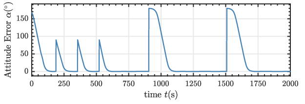
Fig(7) displays the attitude pointing error during the inspection mission. Fig(8) shows the three axis angular velocity of the service and it can be observed that the angular velocity is constrained to be in the range of about $\left[-1.4,1.4\right]^{\circ}/$s.

Fig(9) gives information about the attitude CBFs: 1) in the subgraph above, the availability of the star trackers is listed and it can be concluded that at least one star tracker is available all the time; 2) in the subgraph below, the details of the minimum $h_{ai}$ are shown and the value is 0.0011785, which means that the attitude constraints are satisfied during the whole inspection mission.

From Fig(6) and Fig(9), we can conclude that the position and attitude constraints are satisfied by the proposed controller, which illustrate the effectiveness of the control strategy. Besides, Fig(5) and Fig(8) display that the position and attitude velocity can also be constraint in a certain range, which is smaller than $\boldsymbol{v}_{\max}$ and $\boldsymbol{\omega}_{\max}$. This is because of the term $\alpha_{a}$ and $\alpha_{p}$ in the controllers. In fact, the desired safe velocities for attitude and position controller can be regarded as $\frac{k_{a2}}{k_{a2}+\alpha_{a}}\boldsymbol{\omega}_{s}$ and $\frac{k_{p2}}{k_{p2}+\alpha_{p}}\boldsymbol{v}_{s}$, which means that the designed controller can also restrict the velocities by tracking scaled safe velocities.

References

- Day and Robinson [2020] Day, J. W., and Robinson, S. K., “Two-Fault Tolerant Cold Gas Propulsion System for Spacecraft-Inspection CubeSat,” AIAA Scitech 2020 Forum, American Institute of Aeronautics and Astronautics, 2020. 10.2514/6.2020-1665.
- Nakka et al. [2022] Nakka, Y. K., Hönig, W., Choi, C., Harvard, A., Rahmani, A., and Chung, S.-J., “Information-based guidance and control architecture for multi-spacecraft on-orbit inspection,” Journal of Guidance, Control, and Dynamics, 2022, pp. 1–18. 10.2514/1.g006278.
- Faghihi et al. [2023] Faghihi, S., Tavana, S., and de Ruiter, A. H., “Multiple spacecraft coordination and motion planning for full-coverage inspection of large complex space structures,” Acta Astronautica, Vol. 202, 2023, pp. 119–129. 10.1016/j.actaastro.2022.10.018.
- Capolupo and Labourdette [2019] Capolupo, F., and Labourdette, P., “Receding-horizon trajectory planning algorithm for passively safe on-orbit inspection missions,” Journal of Guidance, Control, and Dynamics, Vol. 42, No. 5, 2019, pp. 1023–1032. 10.2514/1.g003736.
- Fu et al. [2022] Fu, J., Chen, L., Zhang, D., Zhang, J., and Shao, X., “Disturbance Observer-Based Prescribed Performance Predictive Control for Spacecraft On-Orbit Inspection,” Journal of Guidance, Control, and Dynamics, Vol. 45, No. 10, 2022, pp. 1873–1889. 10.2514/1.g006406.
- Weiss et al. [2015] Weiss, A., Baldwin, M., Erwin, R. S., and Kolmanovsky, I., “Model predictive control for spacecraft rendezvous and docking: Strategies for handling constraints and case studies,” IEEE Transactions on Control Systems Technology, Vol. 23, No. 4, 2015, pp. 1638–1647. 10.1109/tcst.2014.2379639.
- Fear and Lightsey [2022] Fear, A., and Lightsey, E. G., “Implementation of Small Satellite Autonomous Rendezvous Using Model Predictive Control,” AIAA SCITECH 2022 Forum, 2022, p. 0838. 10.2514/6.2022-0838.
- Specht et al. [2023] Specht, C., Bishnoi, A., and Lampariello, R., “Autonomous Spacecraft Rendezvous using Tube-based Model Predictive Control: Design and Application,” Journal of Guidance, Control, and Dynamics, 2023. 10.2514/1.g007280.
- Dai and Sun [2015] Dai, R., and Sun, C., “Path planning of spatial rigid motion with constrained attitude,” Journal of Guidance, Control, and Dynamics, Vol. 38, No. 8, 2015, pp. 1356–1365. 10.2514/1.g000705.
- Kjellberg and Lightsey [2013] Kjellberg, H. C., and Lightsey, E. G., “Discretized constrained attitude pathfinding and control for satellites,” Journal of Guidance, Control, and Dynamics, Vol. 36, No. 5, 2013, pp. 1301–1309. 10.2514/1.60189.
- Biggs and Colley [2016] Biggs, J. D., and Colley, L., “Geometric attitude motion planning for spacecraft with pointing and actuator constraints,” Journal of Guidance, Control, and Dynamics, Vol. 39, No. 7, 2016, pp. 1672–1677. 10.2514/1.g001514.
- Wang et al. [2022] Wang, L., Guo, Y., Ma, G., and Zhang, H., “Artificial potential function based spacecraft proximity maneuver 6-DOF control under multiple pyramid-type constraints,” ISA transactions, Vol. 126, 2022, pp. 316–325. 10.1016/j.isatra.2021.08.003.
- Hwang et al. [2022] Hwang, J., Lee, J., and Park, C., “Collision avoidance control for formation flying of multiple spacecraft using artificial potential field,” Advances in Space Research, Vol. 69, No. 5, 2022, pp. 2197–2209. 10.1016/j.asr.2021.12.015.
- Lin et al. [2022] Lin, Z., Wu, B., and Wang, D., “Specific Tracking Control of Rotating Target Spacecraft Under Safe Motion Constraints,” IEEE Transactions on Aerospace and Electronic Systems, 2022. 10.1109/taes.2022.3214799.
- Shao et al. [2022] Shao, X., Hu, Q., Zhu, Z. H., and Zhang, Y., “Fault-tolerant reduced-attitude control for spacecraft constrained boresight reorientation,” Journal of Guidance, Control, and Dynamics, Vol. 45, No. 8, 2022, pp. 1481–1495. 10.2514/1.g006651.
- Menegatti et al. [2022] Menegatti, D., Giuseppi, A., and Pietrabissa, A., “Model Predictive Control for Collision-free Spacecraft Formation with Artificial Potential Functions,” 2022 30th Mediterranean Conference on Control and Automation (MED), IEEE, 2022, pp. 564–570. 10.1109/med54222.2022.9837252.
- Celani and Lucarelli [2020] Celani, F., and Lucarelli, D., “Spacecraft attitude motion planning using gradient-based optimization,” Journal of Guidance, Control, and Dynamics, Vol. 43, No. 1, 2020, pp. 140–145. 10.2514/1.g004531.
- Breeden and Panagou [2021] Breeden, J., and Panagou, D., “Guaranteed safe spacecraft docking with control barrier functions,” IEEE Control Systems Letters, Vol. 6, 2021, pp. 2000–2005. 10.1109/lcsys.2021.3136813.
- Molnar et al. [2021] Molnar, T. G., Cosner, R. K., Singletary, A. W., Ubellacker, W., and Ames, A. D., “Model-free safety-critical control for robotic systems,” IEEE robotics and automation letters, Vol. 7, No. 2, 2021, pp. 944–951. 10.1109/lra.2021.3135569.
- Singletary et al. [2021] Singletary, A., Kolathaya, S., and Ames, A. D., “Safety-critical kinematic control of robotic systems,” IEEE Control Systems Letters, Vol. 6, 2021, pp. 139–144. 10.1109/lcsys.2021.3050609.
- Ames et al. [2019] Ames, A. D., Coogan, S., Egerstedt, M., Notomista, G., Sreenath, K., and Tabuada, P., “Control barrier functions: Theory and applications,” 2019 18th European control conference (ECC), IEEE, 2019, pp. 3420–3431. 10.23919/ecc.2019.8796030.
- Dong et al. [2017] Dong, H., Hu, Q., and Akella, M. R., “Safety control for spacecraft autonomous rendezvous and docking under motion constraints,” Journal of Guidance, Control, and Dynamics, Vol. 40, No. 7, 2017, pp. 1680–1692. 10.2514/1.g002322.
- Chaturvedi et al. [2011] Chaturvedi, N. A., Sanyal, A. K., and McClamroch, N. H., “Rigid-body attitude control,” IEEE control systems magazine, Vol. 31, No. 3, 2011, pp. 30–51. 10.1109/mcs.2011.940459.
- Glotfelter et al. [2018] Glotfelter, P., Cortés, J., and Egerstedt, M., “Boolean composability of constraints and control synthesis for multi-robot systems via nonsmooth control barrier functions,” 2018 IEEE Conference on Control Technology and Applications (CCTA), IEEE, 2018, pp. 897–902. 10.1109/ccta.2018.8511471.
- Li et al. [2014] Li, S., Yang, J., Chen, W.-H., and Chen, X., Disturbance observer-based control: methods and applications, CRC press, 2014. 10.1201/b16570-14.
- Ge and Wang [2004] Ge, S. S., and Wang, C., “Adaptive neural control of uncertain MIMO nonlinear systems,” IEEE Transactions on Neural Networks, Vol. 15, No. 3, 2004, pp. 674–692. 10.1109/tnn.2004.826130.