2021 occultations and transits of Linus orbiting (22) Kalliope: I. Polygonal and ‘cliptracing’ algorithms
Abstract
Aims. The satellite Linus orbiting the main-belt asteroid (22) Kalliope exhibited mutual occultation and transit events in late 2021. A photometric campaign was organized and observations were taken by the TRAPPIST-South, SPECULOOS-Artemis, OWL-Net, and BOAO telescopes, with the goal to further constrain dynamical and photometric models of this sizeable asteroid–satellite system.
Methods. Our dynamical model is sufficiently complex, with multipoles (up to the order ), internal tides, and external tides. The model was constrained by astrometry (spanning 2001–2021), occultations, adaptive-optics imaging, calibrated photometry, as well as relative photometry. Our photometric model was substantially improved. A new precise () light curve algorithm was implemented, based on polygon intersections, which are computed exactly — by including partial eclipses and partial visibility of polygons. Moreover, we implemented a ‘cliptracing’ algorithm, based again on polygon intersections, in which partial contributions to individual pixels are computed exactly. Both synthetic light curves and synthetic images are then very smooth.
Results. Based on our combined solution, we confirmed the size of Linus, . However, this solution exhibits some tension between the light curves and the PISCO speckle-interferometry dataset, acquired contemporarily with the 2021 events. This indicates that improvements of the shape are still possible. In most solutions, Linus is darker than Kalliope, with the single-scattering albedos vs. . This is confirmed on deconvolved images. A detailed revision of astrometric data allowed us to revise also the value of Kalliope. Most importantly, a homogeneous body is excluded. For a differentiated body, two solutions exist: low-oblateness (), with a spherical iron core, and alternatively, high-oblateness () with an elongated iron core. These correspond to the low- and high-energy collisions, respectively, studied by means of SPH simulations in our previous work.
Key Words.
Minor planets, asteroids: individual: (22) Kalliope – Planets and satellites: individual: Linus – Celestial mechanics – Methods: numerical1 Introduction
Mutual events between asteroids and their satellites are not rare (e.g., Pravec & Hahn 1997; Ragozzine & Brown 2009; Wong & Brown 2019; Scheirich & Pravec 2022). The timings of occultations, transits, or eclipses can be used for various precise measurements. Recently, such timings were used to measure the outcome of the DART experiment (Cheng et al. 2018; Statler et al. 2022; Thomas & et al. 2023).
The (22) Kalliope and Linus binary system exhibited the eclipse events back in 2007 (Descamps et al. 2008). With the shape of Kalliope derived from light curves, and an assumed spherical shape of Linus, they obtained its size , based on magnitude drops due to eclipses. This value is compatible with the shadow of Linus, which was observed during the stellar occultation event on Nov 7th 2006.
Here we use more complex dynamical and photometric models of the (22) Kalliope and Linus system to interpret 2021 mutual occultation and transit events. At the same time, our preferred shape model was constrained by the VLT/SPHERE high-resolution AO imaging (Ferrais et al. 2022). Last but not least, a new context has been set up by the discovery of the first M-type Kalliope family (Brož et al. 2022a), which strongly suggests a differentiated interior.
The paper is organized as follows. In Sec. 2, new light curve data are presented, together with other data used to constrain the model. In Sec. 3, a new polygonal light curve algorithm is described. It is generally needed to achieve high precision (), whenever a moon is relatively small, or signal to noise is relatively high. In Sec. 4, a ‘cliptracing’ is described, which is used to compute as-smooth-as-possible synthetic images. Additionally, in Sec. 5, a stellar occultation algorithm is also explained. In Sec. 6, results of our astrometric and photometric models are presented.
2 Observational data
2.1 New light curves
We obtained a calibrated photometry in the Rc band at the 0.6-m TRAPPIST-South telescope (Jehin et al. 2011) and in the custom ‘z cut’ filter at the 1-m Artemis telescope (Burdanov et al. 2022) of the SPECULOOS network (Delrez et al. 2018). The narrow-band ‘z cut’ filter (transmittance from 860 nm to 1100 nm) was used to avoid saturation of the CCD pixels and to suppress the effect of atmospheric water absorption. The relative precision of these data is about . Additional offsets are present between individual nights, which cannot be explained by the variable distance or the phase curve. Hence, the absolute precision is (at worst) .
Out of all light curves, the first one includes a total occultation of Linus. The second is a total transit of Linus. The third is a partial transit of Linus, when only a dark part of (22) was hidden. The fourth is a partial occultation of Linus, when approximately half of Linus was hidden. The event times were prediced using the ephemeris from Ferrais et al. 2022.
We also obtained a relative photometry in the Rc band at the 1.6-m OWL-Net (Park et al. 2018) and 1.8-m BOAO (Sung et al. 2012) telescopes. The data from 2459557, 2459559 were removed, because signal to noise was worse due to weather conditions.
Additional dense light curves were taken from the DAMIT database (Ďurech et al. 2010), in particular 2454175, 2455965, and additional reference light curve from 2459711, was obtained by the BlueEye600 telescope (Ďurech et al. 2018) to constrain the rotation phase.
Light curves from the previous series of events (Descamps et al. 2008) was also used, in particular 2454167, 2454176, (denoted as ‘16’, ‘25’ by Descamps et al. 2008), together with their reference curves (‘14’, ‘27’). They include a total eclipse of Linus, and an annular eclipse of Kalliope. These data were precisely digitized from figures. All data were consistently converted from the UTC to the TDB time scale. The summary of observational circumstances is presented in Tab. 1.
2.2 Calibrated photometry
Moreover, we used sparse calibrated photometry from Gaia (Gaia Collaboration et al. 2018), namely 19 points, with a precision. They were transformed from G to V as follows (van Leeuwen et al. 2018):
| (1) |
where , , , , and was taken from Lupishko et al. 1982. In order to interpret these high-precision data, a precise shape model of (22) is necessary; otherwise the phase curve could not be fitted at all. The data from 2457865.8993, 2457886.9754 were removed from the fit, because they were too offset with respect to the neighbouring points.
In order to extend the phase coverage, from up to , we also included the calibrated UBV photometry from Gehrels & Owings 1962, Scaltriti et al. 1978, Surdej et al. 1986.
2.3 Astrometry
All astrometric data were summarized in Ferrais et al. 2022. In this work, SCAM, PHARO, IRCAL, NIRC2, NACO, NIRI, BTA, SOR, SPHERE, and PISCO datasets were used. Out of the Keck/NIRC2 dataset, four close-in-time measurements, 2452270, 2452270, 2452270, 2452270, were removed from the fit, because they exhibited a systematic photocentre offset. We checked the original images, which were fuzzy due to tracking problems. (Actually, two Linuses were present on one image!)
The astrometry of Descamps et al. 2008, inferred from the eclipse events, 2454167, 2454167, 2454176, 2454176, was removed due to unrealistic uncertainties, which were certainly correlated with the shape. Yet, the shape was somewhat uncertain at that time (cf. their Fig. 2 and Ferrais et al. 2022).
The C2PU/PISCO dataset (Scardia et al. 2019), measured by speckle interferometry, is important because it is temporarily close to the 2021 events. The data from 2459580.6281 was removed due to a substantial offset with respect to the neighbouring points.
Photocentre-to-centre-of-mass corrections were derived from our photometric model (Sec. 3), and applied consistently to all astrometric data.
2.4 AO imaging
The AO imaging by the VLT/SPHERE/ZIMPOL was already described in Ferrais et al. 2022. In this work, 35 deconvolved images were used to obtain observed silhouettes and to constrain the orientation of (22), or to prevent unwanted pole orientations. The uncertainty of silhouettes was nominally assumed ; the pixel scale is , so it corresponds to a sub-pixel precision. It is a very useful regularisation of our dynamical model, because it is sensitive to the inclination of Linus’ orbit with respect to the equator of (22).
Moreover, some of the deconvolved images include Linus itself, in the limited field of view. This can be used to constrain the albedos of both bodies, or whether Linus is darker (or brighter) than (22) Kalliope.
2.5 Stellar occultations
The occultation of (22) Kalliope was already used to refine the shape model (Ferrais et al. 2022). Here we use the most precise astrometric position inferred from the Nov 7th 2006 occultation, which included also Linus (Descamps et al. 2008). In this case, the astrometry is free from any photocentre offsets.
Another Mar 2nd 2022 occultation did not include Linus, unfortunately. For (22) Kalliope, only minor systematic differences at the limb were apparent, with respect to the nominal shape model.
2.6 Shape model
In this work, we use the ADAM shape model from our previous work (Ferrais et al. 2022). It was well-constrained by the AO imaging, light curves, and occultations. However, it could be revised if the pole inferred from dynamics is significantly different from the nominal pole (, ). For a homogeneous body, the oblateness is .
This shape was derived with a regularisation of the centre of mass and the moment of inertia tensor, in order to enforce a rotation about the principal axis. The respective photometry is thus insensitive to any offsets of the centre of mass; it is like with re-centring.
However, there are possible offsets due to the inhomogeneous structure. Hydrodynamic simulations of collisions with a differentiated body described in Brož et al. 2022a, suggest mantle ejection, core deformation, gravitational reaccumulation, and asymmetric deposition (cf. 2 hills, elongated core). Consequently, centre-of-mass offsets will be eventually treated as free parameters.
2.7 Scattering law
Initially, we assumed the Hapke scattering law (Hapke 1981), with parameters similar as for (216) Kleopatra, which is also also an M-type (Descamps et al. 2008). Namely, the opposition effect amplitude , the o. e. width , the asymmetry factor , the roughness .
However, preliminary tests showed that the roughness must be , otherwise the light curve is too curved. We thus preferred roughness from Spjuth 2009, their Tab. 6.3, for (2867) Šteins, .
For the phase curve fitting, we also need the spectral slope between V, Rc bands. This value was derived from the observed spectra of (22) Kalliope (DeMeo et al. 2009).
| Time | Set | Event | Filter | Reference |
|---|---|---|---|---|
| 2454165.5 | ref. | R | Descamps et al. 2008 | |
| 2454167.5 | ecl. of L. | R | Descamps et al. 2008 | |
| 2454175.3 | ref. | R | Hanuš et al. 2016 | |
| 2454176.5 | ecl. of (22) | R | Descamps et al. 2008 | |
| 2454177.5 | ref. | R | Descamps et al. 2008 | |
| 2455965.4 | ref. | R | Vernazza et al. 2021 | |
| 2459546.0 | 9 | ref. | Rc | BOAO |
| 2459546.6 | 13 | occ. of L. | Rc | OWL-Net, Mt. Lemmon |
| 2459546.9 | 1 | occ. of L. | Rc | TRAPPIST-South |
| 2459547.1 | 10 | ref. | Rc | BOAO |
| 2459547.7 | 2 | ref. | Rc | TRAPPIST-South |
| 2459548.5 | 3 | tra. of L. | z cut | SPECULOOS-Artemis |
| 2459548.6 | 4 | ref. | z cut | SPECULOOS-Artemis |
| 2459551.9 | 15 | tra. of L. | Rc | OWL-Net, Mt. Bohyun |
| 2459553.6 | 14 | occ. of L. | Rc | OWL-Net, Mt. Lemmon |
| 2459555.6 | 5 | tra. of L. | Rc | TRAPPIST-South |
| 2459556.7 | 6 | ref. | Rc | TRAPPIST-South |
| 2459557.4 | 7 | occ. of L. | z cut | SPECULOOS-Artemis |
| 2459559.3 | 8 | tra. of L. | z cut | SPECULOOS-Artemis |
| 2459711.3 | ref. | Rc | BE600 |
3 Polygonal light curve algorithm
First, we implemented a new polygonal light curve algorithm to compute light curves of asteroid–satellite systems as precisely as possible. Apart from a stand-alone Fortran module, it was included in our asteroid modelling tool Xitau22 2 https://sirrah.troja.mff.cuni.cz/~mira/xitau/, The algorithm is based on an analytical computation of polygon intersections (Vatti 1992) and the Clipper2 C++ library33 3 https://github.com/AngusJohnson/Clipper2. This is a similar approach as in the stellar modelling tool Phoebe2 (Prša et al. 2016), but complicated by the fact that we have to compute not only the visibility, but also non-convex shadowing, which is critical for asteroids.
In our model, everything is orbiting, rotating, or being affected by free parameters, including the Sun, Earth, (22), Linus. At every time step, occultations, transits, or eclipses must be computed efficiently and exactly. This includes not only total, but also partial or annular events. Moreover, the algorithm should work even if polygons of the 1st body are several times smaller that those of the 2nd body. Of course, uncertainties of the shape itself cannot be avoided (e.g., sphere vs. icosahedron), but the discretisation errors due to finite number of polygons should be minimized (to ).
In order to obtain 1 light curve point, we thus proceed as follows. At the stellar surface, we compute the monochromatic intensity:
| (2) |
the monochromatic flux:
| (3) |
the monochromatic power:
| (4) |
and the pass-band power:
| (5) |
where denotes the effective passband.
At the asteroid surface, we compute the incoming monochromatic flux:
| (6) |
where denotes the Sun–asteroid distance; the pass-band flux:
| (7) |
the reflectance for the given spectral slope :
| (8) |
and the Lambert law factor:
| (9) |
where denotes the single-particle albedo (at ).
At the observer location, we evaluate the solid angle:
| (10) |
where denotes the asteroid–observer distance; and the pass-band calibration flux:
| (11) |
Originally, the shape model is composed of triangular faces. A scaling of nodes, axis rotations, pole orientations, and relative positions of both (22) and Linus are subsequently computed.
A conversion to sets of polygons is then performed; this is important because a clipping of one triangle by another triangle is one or more polygons. Every set contains polygons . Every polygon contains points . Yet, each set is always located in the same plane, because we retain the original geometry.
The geometry is described by the normals , the centres , and the directional cosines , . The non-illuminated and non-visible polygons won’t be computed ().
The 1st transformation is determined by the asteroidSun unit vector , which determines the new basis:
| (12) |
and the respective coordinates:
| (13) |
To optimize the computation, we perform bounding-box tests. Only if polygons are in proximity, we compute the 2-dimensional shadowing (clipping) with the 3-dimensional back-projection as:
| (14) |
where , and .
The 2nd transformation is determined similarly by the asteroidobserver unit vector , with the same Eq. (13). We then compute the visibility (clipping), and the back-projection, with the same Eq. (14). The surface area of the resulting polygons is computed as:
| (15) |
| (16) |
where is the 1st of the polygon points and , are the 2nd, 3rd, etc. , . The sign test is necessary for small polygons big polygons (or annular eclipses).
The incoming monochromatic flux (in ) is then:
| (17) |
the monochromatic intensity (in ) is determined by the bi-directional scattering function:
| (18) |
depending on the cosines and the phase angle . The outgoing monochromatic flux is:
| (19) |
Finally, the integration over the surface determines the monochromatic luminosity (in ):
| (20) |
the pass-band flux:
| (21) |
and the brightness (in mag):
| (22) |
A 2-sphere test of the algorithm is demonstrated in Fig. 1, and the respective light curve for different discretisations in Fig. 2. A tiny-triangle test (Fig. 3) shows that annular eclipses are computed exactly, even for a coarse discretisation.


4 Cliptracing algorithm
Second, we implemented a new ‘cliptracing’ algorithm, which deals with the discretisation errors of synthetic images. Traditional raytracing algorithms perform an inside-triangle test, and use parameters of the respective triangle. Hereinafter, we compute contributions of polygons to individual pixels exactly.
We define 1 pixel as 1 polygon in the sky-plane coordinates :
| (23) |
where , correspond to the centre of pixel, , to the size of pixel. In a cycle over all non-shadowed visible polygons, we ‘crop’ (intersect) each of them by , and sum individual contributions to 1 pixel, to get the monochromatic luminosity of 1 pixel:
| (24) |
where we used already projected surface area , because in our previous formalism (i.e., Eq. (20)), we multiply by unprojected areas . Everything is computed analytically, no discretisation artefacts, no edge artefacts, and the outcome is a smooth synthetic image (see Figs. 4, 5).
When we compare the synthetic image with the observed one, we have to re-center (with a sub-pixel precision). Let us denote the photocentre of the observed AO image, the photocentre of the synthetic AO image. The cliptracing is therefore computed with a centre shifted to .
An optimisation is performed by using a number of bounding-box tests (namely, the observed bounding-box, the over-all-polygons bounding-box, the 1-pixel bounding-box, and the individual bounding-boxes of polygons).
Another problem we have to deal with at this level of precision, is a correlation of ‘everything’ with the shape. Especially the timings of events depend on details of the shape, henceforth we created a version of our modelling tool focused on the fitting of shape (“Xitaushp”).
The parameters are radius vectors of the ‘control’ shape, which is processed by a sub-division algorithm (Kobbelt 2000; Viikinkoski et al. 2015), with 1 up to 4 levels. The input orbit is read from the previous output, for simplicity.
To constrain the shape, we use a modified metrics:
| (25) |
where the individual contributions (and weights) correspond to the light curves (LC), silhouettes (AO), and synthetic images (AO2). If not stated otherwise, we use unit weights. The computation of silhouettes was already described in Brož et al. 2021. It was improved by a multi-point interpolation, which is smooth even for low resolution, even for deconvolution artefacts, which is occasionally present as a drop of signal at the edge (‘stair case’).
The synthetic image is convolved with the point-spread function (PSF). We use the Moffat PSF:
| (26) |
with free parameters , . Alternatively, an observed stellar PSF can be input; it is rather complex, with the Strehl ratio about 0.1, a diffraction pattern, a ring, a cross, remaining AO artefacts. However, for deconvolved images we would need a ’residual’ PSF instead.
The respective contribution for synthetics images is computed as a sum over pixels:
| (27) |
where denotes the observed monochromatic luminosity, synthetic, the Heaviside step function. The Poisson uncertainty is computed as for each pixel, because sometimes we have to compare to darkness (). The minimum luminosity is computed as for all pixels, because background is rather extended and uneven; the factor (threshold) often corresponds to the silhouettes.
| “cliptracing” | raytracing |
|---|---|
 |
 |
 |
 |
5 Stellar occultation algorithm
Third, we implemented a new occultation algorithm in Xitau. It is used to check the astrometric positions, timings of occultations and precision of the ephemerides. At the beginning, we use a sphere-intersection test to speed-up the computation. We apply a standard TDB to UT1 conversion (IAU SOFA Center 2014), precession (Lieske et al. 1977) nutation (Wahr 1981; Wolf 1992), an equatorial-of-J2000 to equatorial-of-date transformation, a proper motion of the respective star (from the Gaia DR3), and an ellipsoid-intersection test:
| (28) |
| (29) |
namely for the WGS-84 ellipsoid (, ), where denotes the Earthasteroid vector, starasteroid (normalized), the intersection point on the ellipsoid; is a nuisance parameter. The equation is quadratic in . At the end, we apply UT1 to GST conversion, the Earth rotation, and a transformation to the geodetic coordinates:
| (30) |
| (31) |
with an iterative procedure for the inverse.
An example for (22) Kalliope is shown in Fig. 6. The algorithm was verified against selected events from the Occult software (Herald et al. 2020), e.g., the astrometric position of (216) Kleopatra, on Mar 12th 2015 (see Fig. 19).

6 Occultation, transit and eclipse events
Before we proceed with fitting, it is useful to summarize our dynamical model: it uses the Bulirsch–Stoer numerical integrator, adaptive time step, which allows us to compute non-keplerian orbits, multipoles up to the order , internal tides, or external tides by the Sun (Brož 2017; Brož et al. 2021; Brož et al. 2022b). In the nominal model, we assume the tidal time lag inferred for (216) Kleopatra.
Modifications were described in detail in Sects. 3, 4, 5. Explanation of all parameters is included in Tab. 2. In particular, we added a few free parameters, namely , , , , , , , which allowed us to fit the astrometry, light curves, or scattering parameters. Alternatively, we added offsets in , , directions, due to a possible rotation about different axis.
We use several types of observations to constrain the model:
| (32) |
where individual contributions correspond to astrometry (the so-called SKY dataset), silhouettes (AO), light curves (LC), or occultations (OCC); all of them with corresponding weights. Previously, we used so that AO contributes comparably as SKY. Of course, every model requires reasonable initial conditions; therefore we used the best fit from Ferrais et al. 2022, with the osculating elements adjusted to match slightly simplified dynamics (). We verified that omitting high-order terms does not substantially shift the values of low-order terms, in particular, of the oblateness .
6.1 Long-arc scattering model
First, we focused on the phase curve, which is controlled by 6 free parameters , , , , , . We used the calibrated photometry from Gehrels & Owings 1962, Scaltriti et al. 1978, Surdej et al. 1986, this work, and the Gaia DR3 data. The zero points were fixed, however, we expect calibration systematics up to 0.05 mag. A shape model of (22) Kalliope is necessary, because the lightcurve amplitude can reach 0.6 mag, depending on geometry. The simplex and subplex (i.e., simplex on subspaces; Rowan 1990) algorithms were used, with several restarts. The resulting phase curve is shown in Fig. 7.
The model is sensitive mostly to , , scattering parameters. The unreduced is too large compared to the number of observations due to remaining calibration systematics. If 0.05 mag uncertainties are used instead, the decreases down to . Nevertheless, the best-fit values, , , , seem to be reasonable. A correlation exists between , , , because small can be compensated by large , . Hence, the overall uncertainties are increased to 0.10, 0.1, 0.01, respectively. If , are also free, their values tend to converge towards , , which do not seem to be common (cf. Li et al. 2015). In order to fit both the phase curve and the light curve with the given shape of (22), we shall use these values, until we modify the shape (Sec. 6.7). Their uncertainties are of the order of 0.10, , respectively. Detailed light curve shape is also sensitive to , .
6.2 Short-arc scattering model
We fitted details on 2 light curves from SPECULOOS-Artemis (datasets 3, 4), because we have to use calibrated photometry and avoid any zero-point offsets between datasets. (Again, zero points were fixed.) We computed a systematic grid for , parameters, which were kept fixed, while , , , , parameters were free. According to Fig. 8, the fit is still not perfect (, ) partly because everything is interrelated — albedo, scattering, shape, pole, Linus, orbit, occultations, transits, eclipses, etc. It is possible to find solutions for up to , and . Small values of seem to be excluded, because the albedo of Linus is pushed to unrealistic low values. Large values of seem to be excluded, because the light curve amplitude is incorrect (at least for the given shape). Given the preference for negative (Spjuth 2009), we prefer solutions close to , . Alternatively, albedo variegation, or roughness variegation may be present on the surface.
6.3 Short-arc, astrometric + photometric model
As the next step, we fitted 4 light curves from SPECULOOS-Artemis and TRAPPIST-South (datasets 1, 2, 3, 4), together with the PISCO astrometric dataset, which was acquired very close to the occultation and transit events. Also the silhouettes were used to prevent incompatible pole orientations, which influence the events. Analytical zero points were computed, compensating for remaining offsets between the respective light curves. The best-fit total weighted unreduced , with the individual contributions , , and , where the respective numbers of observations , , . The fit exhibits no systematics in astrometry; see Fig. 9. Minor systematics are present in the light curves, (Fig. 10), nevertheless, the amplitude as well as the duration of the occultations and transit events is matched almost perfectly. An example of geometry is shown in Fig. 11.
We checked that a mirror solution (occultationtransit) is not possible; the variable geometry allows to distinguish these solutions.
6.4 Long-arc, astrometric model
In order to constrain the dynamical parameters, astrometric measurements from 2452151 to 2459580 were used, as well as the silhouettes to prevent incompatible pole orientations. In this case, the free parameters were: , , , , , , , , , , while the fixed parameters: , , . Actually, we computed an extended grid for the latter two parameters, in the range of to , to , respectively. Apart from , we included other multipoles up to , which were computed for a homogeneous structure:
A very important result is that two solutions exists for the oblateness , either , or (see Fig. 12). A homogeneous body with is excluded. These two solutions correspond to 3 or 2 nodal precession cycles (see, e.g., Fig. 16). There is no other option (4 or 1 cycle), because would be unrealistic (too high or too low). The best-fit value is , or alternatively . It indicates no systematics, possibly overestimated uncertainties, because the number of data points is (both , ).
We also checked a range of , values (Fig. 20). We tested mirror solutions, retrograde solutions, shifted-by- solutions. There is no alternative solution, neither for the eccentricity, nor for the inclination. The uncertainties are up to (in log-scale), .
6.5 Long-arc, astrometric + photometric model
In order to constrain the physical parameters, 4 light curves (datasets 1, 2, 3, 4), all astrometric measurements, and all silhouettes were used. Apart from dynamical parameters, additional free parameters , , , can be now constrained by mutual occultation and transit events. We fixed the parameters: , , , , , otherwise the model would not match the calibrated photometry (Sec. 6.1). Again a grid of , was computed (Fig. 13).
The best-fit , with the individual contributions , , and . All of them are slightly worse, most likely due to a combination of more observational datasets, but it is an acceptable compromise.
Regarding the oblateness, seems to be a bit more compatible with the light curves, but we still cannot exclude the solution. The tidal time lag is not well constrained. The volume-equivalent diameters of (22), , is still compatible with the ADAM or MPCD shapes (Ferrais et al. 2022); the uncertainty is of the order of .
A specific grid was computed for , of Linus (Fig. 14). It further improved . In this particular model, , with a similar uncertainty. It is compatible with the stellar occultation observed on Nov 7th 2006 (Descamps et al. 2008). All parameters of this model are presented in Tab. 2. The global uncertainties of parameters were estimated from a series of alternative admissible solutions (cf. models above; Figs. 12, 13, 14). In this order-of-magnitude estimate, we included also a contribution from systematic uncertainties. We verified these results by using all available light curves (from Tab. 1), which resulted in a statistically equivalent model (cf. Tab. 3). The Markov Chain Monte Carlo (MCMC) simulation is presented in Fig. 21; it demonstrates typical local uncertainties and correlations in the surroundings of one local minimum (close to ).
The Linus’ orbit, together with available astrometric measurements, is shown in Fig. 15. It was checked by the stellar occultation computation (Fig. 6). The temporal evolution of osculating elements is demonstrated in Fig. 16.
In most solutions, Linus seems to be darker compared to (22), the single-scattering albedo is , , respectively, with the local uncertainties of the order of . They are naturally correlated. The darkness is also apparent on those deconvolved AO images, which capture both (22) and Linus at the same time. The appearance is only partly affected by a difference between (more) flat vs. (more) curved surface.
Finally, we should not be misled by sparse local minima, which are relatively deep; they compensate some systematics on the light curve which are however unrelated to the mutual occultation or transit events. Yet, such solutions are in contradiction with the PISCO astrometric dataset; see Fig. 15. We thus prefer solutions, which fit the orbit just prior/posterior of the events. Possibly, the shape of (22) Kalliope should be also adjusted.
| nominal | high-oblateness | |||
| var. | val. | val. | unit | |
| 1 | ||||
| day | ||||
| 1 | ||||
| deg | ||||
| deg | ||||
| deg | ||||
| deg | ||||
| 76.5 km | ||||
| 15 km | ||||
| day | ||||
| day | ||||
| s | ||||
| 1 | ||||
| deg | ||||
| deg | ||||
| deg | ||||
| – | 1 | |||
| – | 1 | |||
| – | 1 | |||
| – | 1 | |||
| – | 1 | |||
| – | deg | |||
| 344 | 344 | |||
| 12600 | 12600 | |||
| 1829 | – | |||
| 14773 | 12944 | |||
| 364 | 249 | |||
| 35209 | 36818 | |||
| 6223 | – | |||
| 6695 | 359 |
6.6 Possible centre-of-mass offset of (22)
The simplest adjustment is a centre-of-mass offset due to an asymmetric internal structure. This implies rotation about a different axis and different extent of the central body in different directions. Because the orbit of Linus is well constrained by astrometry, the timings of mutual occultations or transits offer an opportunity to measure the offset not directly (in space), but indirectly (in time).
Therefore, we added three more free parameters to our model, the offsets in , , or directions. After testing values up to , which did affect substantially, we conclude that it did not converge to a unique significant minimum. We thus have to look for a more complex solution.
6.7 Possible shape adjustment of (22)
In order to have a full control, we derived a new shape model of (22) Kalliope. We started with a low-resolution ellipsoid, (with the number of nodes ), which serves as a ‘control’ shape. After 3 sub-divisions, we obtained a high-resolution shape (), which was converged and constrained by AO silhouettes as well as light curves. We used no additional regularisation term in our metric. Nevertheless, we assured that is indeed sensitive to all shape parameters.
In order to capture fine details, we used the medium-resolution (22)-like shape (), after the 1st subdivision. After 2 more sub-divisions, we again obtained a high-resolution shape, which was constrained by AO images and light curves.
In particular, we converged the following free parameters: radii of control nodes, , , , , , , , , with several restarts of simplex or subplex. The best-fit shape model is shown in Fig. 17.
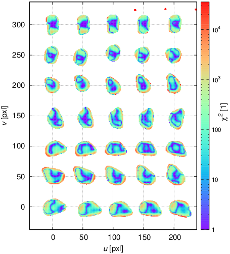
The total signal contained in all pixels in all images is ‘huge’, the unreduced , while the number of points (pixels) taken into account is . This is at least partly due to rotation, which changes the projected shape during an exposure in a non-trivial way, remaining deconvolution artefacts, present on images taken at 2458643, 2458661, 2458672, or relatively low background level on the same set of images.
Overall, our new shape is still similar to the ADAM model (Fig. 5), and it is even more so in the line-of-sights projections. However, it is fine-tuned to the respective datasets, with the respective contributions, vs. , vs. , significantly improved. Systematics on the light curves related to the shape were at least partly eliminated (cf. Fig. 4).
In principle, one should use this shape and start over again (from Sect. 6.1, 6.2, …). While it is not beyond the scope of this paper, we postpone such an in-depth study — including optimisations of ‘everything’ together with shape — as a future work.


7 Conclusions
In this work, mutual occultation, transit and eclipse events of Linus orbiting (22) Kalliope were used to constrain combined astrometric + photometric models of this binary system. Using innovative algorithms for photometric computations (see Sects. 3, 4), we confirmed the size of Linus , improved the shape of (22) Kalliope, and put strong constraints on its dynamical oblateness.
On one hand, we were not surprised by the low-oblateness () solution, because (22) Kalliope is probably the best candidate for a differentiated body (Vernazza et al. 2021). At the same time, the iron core is usually considered to be more-or-less spherical, because this is a standard outcome of differentiation.
On the other hand, we were surprised by the second, high-oblateness () solution. Surprisingly, it should correspond to an irregular (or highly ellipsoidal) iron core. In fact, (22) Kalliope suffered a major collision about 900 My ago, which gave birth to the Kalliope family (Brož et al. 2022a). Some of the SPH simulations of this event, we performed in our previous work, indicate that the iron core of the original body is deformed and even elongated, especially in medium- to high-energy collisions (with the projectile size ). One example is shown in Fig. 18.
In the future, it should be possible to distinguish these two solutions by new astrometric (imaging or speckle-interferometric) observations, obtained at a suitable phase(s) of the precession cycle (seen, e.g., in Fig. 16).

Acknowledgements.
This work has been supported by the Czech Science Foundation through grants 21-11058S (M. Brož), 20-08218S (J. Ďurech, J. Hanuš). In this work, measurements from the BlueEye600 telescope, supported by the Charles University, were used. The TRAPPIST is a project funded by the Belgian Fonds (National) de la Recherche Scientifique (F.R.S.-FNRS) under grant PDR T.0120.21. J. de Wit and MIT gratefully acknowledge financial support from the Heising-Simons Foundation, Dr. and Mrs. Colin Masson and Dr. Peter A. Gilman for Artemis, the first telescope of the SPECULOOS network situated in Tenerife, Spain. We also thank an anonymous referee for constructive comments.References
- Brož (2017) Brož, M. 2017, ApJS, 230, 19
- Brož et al. (2022a) Brož, M., Ferrais, M., Vernazza, P., Ševeček, P., & Jutzi, M. 2022a, A&A, 664, A69
- Brož et al. (2021) Brož, M., Marchis, F., Jorda, L., et al. 2021, A&A, 653, A56
- Brož et al. (2022b) Brož, M., Ďurech, J., Carry, B., et al. 2022b, A&A, 657, A76
- Burdanov et al. (2022) Burdanov, A. Y., de Wit, J., Gillon, M., et al. 2022, PASP, 134, 105001
- Cheng et al. (2018) Cheng, A. F., Rivkin, A. S., Michel, P., et al. 2018, Planet. Space Sci., 157, 104
- Delrez et al. (2018) Delrez, L., Gillon, M., Queloz, D., et al. 2018, in Society of Photo-Optical Instrumentation Engineers (SPIE) Conference Series, Vol. 10700, Ground-based and Airborne Telescopes VII, ed. H. K. Marshall & J. Spyromilio, 107001I
- DeMeo et al. (2009) DeMeo, F. E., Binzel, R. P., Slivan, S. M., & Bus, S. J. 2009, Icarus, 202, 160
- Descamps et al. (2008) Descamps, P., Marchis, F., Pollock, J., et al. 2008, Icarus, 196, 578
- Ďurech et al. (2018) Ďurech, J., Hanuš, J., Brož, M., et al. 2018, Icarus, 304, 101
- Ďurech et al. (2010) Ďurech, J., Sidorin, V., & Kaasalainen, M. 2010, A&A, 513, A46
- Ferrais et al. (2022) Ferrais, M., Jorda, L., Vernazza, P., et al. 2022, A&A, 662, A71
- Gaia Collaboration et al. (2018) Gaia Collaboration, Brown, A. G. A., Vallenari, A., et al. 2018, A&A, 616, A1
- Gehrels & Owings (1962) Gehrels, T. & Owings, D. 1962, ApJ, 135, 906
- Hanuš et al. (2016) Hanuš, J., Ďurech, J., Oszkiewicz, D. A., et al. 2016, A&A, 586, A108
- Hapke (1981) Hapke, B. 1981, J. Geophys. Res., 86, 3039
- Herald et al. (2019) Herald, D., Frappa, E., Gault, D., et al. 2019, NASA Planetary Data System, 3
- Herald et al. (2020) Herald, D., Gault, D., Anderson, R., et al. 2020, MNRAS, 499, 4570
- IAU SOFA Center (2014) IAU SOFA Center. 2014, SOFA: Standards of Fundamental Astronomy, Astrophysics Source Code Library, record ascl:1403.026
- Jehin et al. (2011) Jehin, E., Gillon, M., Queloz, D., et al. 2011, The Messenger, 145, 2
- Kobbelt (2000) Kobbelt, L. 2000, Proc. Computer graphics and interactive techniques, 103
- Li et al. (2015) Li, J. Y., Helfenstein, P., Buratti, B., Takir, D., & Clark, B. E. 2015, in Asteroids IV, 129–150
- Lieske et al. (1977) Lieske, J. H., Lederle, T., Fricke, W., & Morando, B. 1977, A&A, 58, 1
- Lupishko et al. (1982) Lupishko, D. F., Belskaia, I. N., Tupieva, F. A., & Chernova, G. P. 1982, Astronomicheskii Vestnik, 16, 101
- Park et al. (2018) Park, J.-H., Yim, H.-S., Choi, Y.-J., et al. 2018, Advances in Space Research, 62, 152
- Pravec & Hahn (1997) Pravec, P. & Hahn, G. 1997, Icarus, 127, 431
- Prša et al. (2016) Prša, A., Conroy, K. E., Horvat, M., et al. 2016, ApJS, 227, 29
- Ragozzine & Brown (2009) Ragozzine, D. & Brown, M. E. 2009, AJ, 137, 4766
- Rowan (1990) Rowan, N. 1990, Ph.D. thesis, Univ. Texas Austin
- Scaltriti et al. (1978) Scaltriti, F., Zappala, V., & Stanzel, R. 1978, Icarus, 34, 93
- Scardia et al. (2019) Scardia, M., Rivet, J.-P., Prieur, J.-L., et al. 2019, Astronomische Nachrichten, 340, 771
- Scheirich & Pravec (2022) Scheirich, P. & Pravec, P. 2022, Planet. Sci. J., 3, 163
- Spjuth (2009) Spjuth, S. 2009, PhD thesis, Technical University of Braunschweig, Germany
- Statler et al. (2022) Statler, T. S., Raducan, S. D., Barnouin, O. S., et al. 2022, Planet. Sci. J., 3, 244
- Sung et al. (2012) Sung, H.-I., Park, Y.-H., Lee, S.-M., et al. 2012, Publication of Korean Astronomical Society, 27, 95
- Surdej et al. (1986) Surdej, J., Pospieszalska-Surdej, A., Michalowski, T., & Schober, H. J. 1986, A&A, 170, 167
- Thomas & et al. (2023) Thomas, C. & et al. 2023, Nature, in press
- van Leeuwen et al. (2018) van Leeuwen, F., de Bruijne, J. H. J., Arenou, F., et al. 2018, Gaia DR2 documentation, Gaia DR2 documentation, European Space Agency; Gaia Data Processing and Analysis Consortium.
- Vatti (1992) Vatti, B. R. 1992, Comm. ACM, 35, 56
- Vernazza et al. (2021) Vernazza, P., Ferrais, M., Jorda, L., et al. 2021, A&A, 654, A56
- Viikinkoski et al. (2015) Viikinkoski, M., Kaasalainen, M., & Durech, J. 2015, A&A, 576, A8
- Wahr (1981) Wahr, J. M. 1981, Geophysical Journal, 64, 705
- Wolf (1992) Wolf, M. 1992, Astronomická příručka (Academia)
- Wong & Brown (2019) Wong, I. & Brown, M. E. 2019, AJ, 157, 203
Appendix A Supplementary figures
Stellar occultation algorithm verification for (216) Kleopatra is show in Fig. 19. Additional models from Sec. 6.4 are shown in Fig. 20. The corner plot discussed in Sec. 6.5 si shown in Fig. 21. The adjusted shape model and the respective light curve fit discussed in Sec. 6.7 is shown in Figs. 5, 4. Additional best-fit model is presented in Tab. 3.


| all-data | ||
| var. | val. | unit |
| 1 | ||
| day | ||
| 1 | ||
| deg | ||
| deg | ||
| deg | ||
| deg | ||
| 76.5 km | ||
| 15 km | ||
| day | ||
| day | ||
| s | ||
| 1 | ||
| deg | ||
| deg | ||
| deg | ||
| 1 | ||
| 1 | ||
| 1 | ||
| 1 | ||
| 1 | ||
| deg | ||
| 344 | ||
| 12600 | ||
| 6852 | ||
| 19796 | ||
| 321 | ||
| 36108 | ||
| 52482 | ||
| 59313 |