Towards Better Explanations for Object Detection
Abstract
Recent advances in Artificial Intelligence (AI) technology have promoted their use in almost every field. The growing complexity of deep neural networks (DNNs) makes it increasingly difficult and important to explain the inner workings and decisions of the network. However, most current techniques for explaining DNNs focus mainly on interpreting classification tasks. This paper proposes a method to explain the decision for any object detection model called D-CLOSE. To closely track the model’s behavior, we used multiple levels of segmentation on the image and a process to combine them. We performed tests on the MS-COCO dataset with the YOLOX model, which shows that our method outperforms D-RISE and can give a better quality and less noise explanation.
1 Introduction
Lately, deep neural networks (DNNs) in object detection for images have become popular because of their superior performance in several domains, such as healthcare miotto2018deep; nguyen2023towards and self-driving cars do2018real. However, the lack of transparency in decision-making leads to suspicion among end-users, which could negatively affect the widespread AI applications, especially in areas that require trust from users. Furthermore, newer regulations like the European General Data Protection Regulation (GDPR) regulation2018general strictly require the transparency of using black-box models. Thus, a growing chorus of researchers is calling for eXplainable Artificial Intelligence (XAI) methods. Today, many XAI methods are proposed mainly for classification problems das2020opportunities. However, explaining object detectors is a big challenge due to the structural differences between the classification and object detection models. Several state-of-the-art XAI methods for object detectors are proposed, such as Surrogate Object Detection Explainer (SODEx) sejr2021surrogate and Detector-Randomized Input Sampling for Explanation of Black-box Models (D-RISE) petsiuk2021black. Yet, these methods meet problems in giving interpretable explanations, tuning hyperparameters for each object without a feature regions’ size information, and degraded performance with large datasets.
Hence, in this paper, our main contributions are as follows:
- 1.
We proposed a new agnostic XAI method for object detectors, called Detector-Cascading multiple Levels of Segments to Explain (D-CLOSE). It can explain any object detector’s prediction by giving a saliency map that estimates each pixel’s importance in the input image to the model’s prediction for each individual object.
- 2.
We evaluated the proposed D-CLOSE on the MS-COCO validation dataset lin2014microsoft. Results show that D-CLOSE requires less computation time and provides better performance both in classification and localization than D-RISE, the best XAI method for detector model as for as we know.
- 3.
We proposed quantitative and qualitative evaluations for each object-size group to demonstrate the stability of the methods with large datasets.
- 4.
We analyzed D-CLOSE on four cases of the YOLOX’s prediction errors ge2021yolox on the MS-COCO dataset.
- 5.
We further evaluated D-CLOSE with real-world images affected by bad conditions, images containing overlapping objects, and different spectra images to demonstrate the method’s applicability.
2 Related Work
2.1 Object Detection Model
Object detection is an essential field in computer vision that detects the instances of visual objects of a particular class in digital images. One-stage and two-stage models are the two main approaches to building an object detector zou2019object. One-stage models are often based on fixed grids and make predictions directly from the input image, such as YOLOX ge2021yolox, a recent release in the YOLO series redmon2016you. Primarily, YOLOX uses a decoupled head to avoid the problem of collisions between classification and regression branches that reduce model accuracy. The two-stage model, Faster-RCNN ren2015faster, proposed a set of regions of interest by selected search or Region Proposal Network. The proposed regions are sparse as the potential bounding box candidates can be infinite. Then, another fine-tuned network processes these regional proposals to decide the final prediction.
2.2 Explainable AI
A series of XAI methods were born and divided into two categories based on visualization of the explanations: Pixel-based saliency and Region-based saliency methods hartley2021swag.
2.2.1 Pixel-based Saliency Methods
Pixel-based saliency methods measure each pixel’s significance score in the input by backpropagating from the prediction to the desired class, such as Gradient simonyan2014visualising, LRP bach2015pixel, and Deep Taylor shrikumar2017learning, which focus on explaining classification models. A framework called “Explain to Fix” gudovskiy2018explain, based on Shapley Additive Explanation (SHAP) lundberg2017unified, was proposed to extend the applicability of these methods to object detection problems. Later, Contrastive Relevance Propagation tsunakawa2019contrastive, an extension of the LRP method, was proposed to explain the output decisions of the Single-Shot Object Detector liu2016ssd by scoring for object classes and offsets in bounding box locations and generating heatmaps highlighting the inputs that contribute significantly to the output. However, pixel-based saliency methods, where pixels are scored separately, are often less interpretable wagner2019interpretable.
2.2.2 Region-based Saliency Methods
Region-based saliency methods usually provide a heatmap or regions in the input image representing the key factors contributing to the model’s predictions. Hence, its explanation is comprehensible to end-users rather than optimizing the accuracy of the explanation on individual pixels cooper2021believe. The first studies showed that the final activation layers often carry complete feature information, which is the main basis for final predictions zhou2016learning; selvaraju2017grad, so several Class Activation Mapping (CAM)-based methodszhou2016learning; selvaraju2017grad; chattopadhay2018grad; nguyen2022secam are proposed to calculate the importance of each feature map in the final activation layer of classification models. Instead of using only one final convolutional layer, Semantic Input Sampling for Explanation (SISE) sudhakar2021ada uses multiple intermediate convolutional layers to provide better spatial resolution and completeness of the explanation.
Other techniques aim to interpret any model regardless of the model’s architecture. For instance, Local Interpretable Model-agnostic Explanations (LIME) ribeiro2016should generates perturbations from subdivided superpixels from the image, then computes the output values and fits into a single regression model to calculate the weights. Another method using input noise for sampling is Randomized Input Sampling for Explanation of Black-box Models (RISE) petsiuk2018rise, which generates random perturbation masks and transitions through the model, taking the predicted probabilities for the target class as weights for those masks. Morphological Fragmental Perturbation Pyramid for Black-Box Model Explanations (MFPP) yang2021mfpp generates a saliency map using multiple levels of superpixels kapishnikov2019xrai to sample perturbations and then combines them.
An advantage of utilizing region-based methods is their explanation for model object detectors. Object detectors’ output, classification and localization, need some different techniques to explain them. Furthermore, most object detectors do not use fully connected (FC) layers but convolutional layers, resulting in the “receptive field” of the target output being only part of the input image rather than the entire image as in the classification task xia2021receptive. To our knowledge, there are currently Surrogate Object Detection Explainer (SODEx) sejr2021surrogate and Detector-Randomized Input Sampling for Explanation of Black-box Models (D-RISE) petsiuk2021black can explain both one-stage and two-stage object detectors. In detail, SODEx uses Surrogate Binary Classifier to convert object detectors’ outputs, then uses LIME to explain. While SODEx only shows the most important regions based on a segmentation algorithm, D-RISE provides a more intuitive and easier-to-understand explanation as a saliency map. D-RISE leverages the idea from RISE, replacing the weights for each perturbation sample by calculating the similarity between the proposal vectors and the target vector. However, D-RISE has a major disadvantage; namely, tuning hyperparameters for each object is difficult because we cannot know the size of the feature regions, which causes great obstacles in model execution and evaluation on a larger dataset. Additionally, methods, like D-RISE, use the way of creating masks from RISE petsiuk2018rise, only gives the best results with rectangular objects; otherwise, D-RISE’s performance degrades because it generates random masks based on the mesh yang2021mfpp.
Hence, we proposed D-CLOSE, a new saliency method that can also interpret any object detector, which is more efficient than D-RISE due to using fewer data samples, saving computational time with superior qualitative and quantitative results.
3 Proposed method
We proposed Detector-Cascading multiple Levels of Segments to Explain (D-CLOSE) to generate saliency maps that can explain the decision of both one-stage and two-stage object detectors. Given input image of size , an object detector , our method generates the explanation for detected objects in seven steps (Sec. 3.5). The overall architecture of D-CLOSE is illustrated in Fig. 1.

3.1 Random masks generation
Images often contain several objects in various sizes and shapes. We were inspired by mask generation from MFPP yang2021mfpp to generate random masks to explain object detectors. We inherit the mask generation approach of MFPP as follows:
- •
We use Simple Linear Iterative Clustering (SLIC) achanta2010slic, a quick method to split the image into superpixels with different levels by changing the number of superpixels [] to segment the image.
- •
We generate binary masks of size by setting the segments to with probability and with the remaining segments.
- •
We upsample all masks using bilinear interpolation as this formula .
- •
We crop masks with uniformly random indents from up to ,.
3.2 Similarity score
The vector that encodes the predictions of the object detection models is as follows:
| (1) |
where:
- •
Detection box (B): coordinates of the predicted objects, is top-left corner, is bottom-right corner
- •
Objectness score (O): is the probability of predicting a bounding box containing any one object
- •
Detection object’s score (C): is the vector representing the correctly predicted scores of the classes in the bounding box.
We calculate the correlation between the target vector and the proposal vectors , then use it as a weight for the mask, which is forwarded into the model petsiuk2021black. We use a similarity score calculation formula from D-RISE:
| (2) |
3.3 Density map
Given an -by-, the mask , is the value of each pixel at position . Randomly generated masks produce a non-uniform distribution. Some maybe appear more, and some appear very little, leading to unfair results. We aggregate all weighted masks with the output prediction forming a density map of size to compute the randomly generated masks’ distribution.
| (3) |
| (4) |
where and are the importance scores of each pixel before and after the processing, respectively. We have found that normalizing the density map can help produce smoother and less noisy explanations (Fig. 2). In addition, we also set up experiments and used metric evaluations to strengthen our argument further (Sec. 5.3).

3.4 Fusion feature map
After normalizing the density map generated from Sec. 3.3, we obtain feature maps corresponding to levels of the superpixel segment. Each feature map interprets the object’s small to large features. Intuitively, small features are the most important to identify the object’s class, while large features contain the generic and relevant context in which the object is found. Our method, inspired by SISE sudhakar2021ada, aggregates feature maps at the semantic level by prioritizing more detailed features and descending to more general features. However, SISE forcibly removes noises using threshold parameters with Otsu’s algorithm otsu1979threshold, making the explanations sometimes confusing to end-users. Additionally, when SISE deals with complex models, selecting the final convolutional layers in the blocks is extremely difficult, especially in object detection problems, because the pooling layers are not at the end of each block. We build a flexible and natural framework (Fig. 3), which does not access model internals, does not use threshold parameters, and can construct a wide range of feature maps with areas from detailed to generic regardless of the model architecture.
3.5 Saliency maps inference
We combine all the above operations as a procedure, including random mask generation, similarity score, density map, and fusion feature map, which can infer saliency maps for any object detector. The procedure is as follows:
- 1.
The input image is divided into levels of segments. Each segmentation level generated perturbation masks , where , .
- 2.
We generate masked images by element-wise masks created with image input ().
- 3.
Masked images are forwarded into the object detectors to get vectors of prediction:
(5) where .
- 4.
We calculate the similarity between target vector to be explained and proposal vectors . Then, we take the maximum score for each masked image on each target vector:
(6) where .
- 5.
We calculate the density map representing the distribution of randomly generated masks in Eq. 3, where .
- 6.
We compute the average score of each pixel by dividing the weighted sum of masks by the density map to obtain the saliency map for the segment level.
(7) where .
- 7.
We combine each semantic level’s saliency maps from the features by cascading in blocks, as shown in Fig. 3. Mathematically, our process works like a recursive algorithm where is the saliency map obtained after each step. In the last step, the saliency map obtained is :
(8)
4 Experiments and results
4.1 Datasets and models
We evaluate our method with a pre-trained YOLOX model ge2021yolox11 1 https://github.com/Megvii-BaseDetection/YOLOX on the MS-COCO validation dataset lin2014microsoft. In quantitative evaluation, results are obtained with the same set of parameters on the same data set. All experiments use Nvidia Tesla T4 and 24GB RAM as the benchmark.
4.2 Parameters setup
For D-RISE, we use default parameters proposed in the original paper with masks, probability and resolution .
For D-CLOSE, during the masking process, we use a segmentation algorithm that splits the image into levels with the number of segments , respectively. For each image, we perform our method with masks per segmentation level, a kernel width , and resize offset ratio .
4.3 Sanity checks
A saliency map can explain which features the model considers to predict and why the model gives the correct explanation or not. Hence, the saliency map reveals the weights that the model learned during training. We use sanity checks adebayo2018sanity to check whether D-CLOSE results faithfully reflect the decision-making behavior of the model. We check whether the saliency map changes by changing the model’s weights. In the experiment, our method’s saliency map shows that the model focuses on another region with altered weights, which means that our method can faithfully reflect the model’s behavior (Fig. 4).


4.4 Model errors
Inspired by hoiem2012diagnosing, we evaluate whether D-CLOSE can generate feature maps that explain the incorrect decisions of the model. We further extend the test case where the model predicts an object that does not exist in the image. Also, we analyze the classification error and localization error of the YOLOX model on the MS-COCO dataset.


We compare the two generated explanations for the ground truth and predicted bounding box, then calculate the difference by subtracting the corresponding pixel values between them. The difference between the two saliency maps can indicate the source of the error.
4.5 Model in images affected by bad conditions
Our experiment utilizes D-CLOSE to explain the model’s detection of images from surveillance cameras that record images of pedestrians and vehicles in bad conditions such as low light, fog, and night. Also, based on bayer2021comparison, we evaluate D-CLOSE with images in different spectra. Test images are obtained from the WIDER Pedestrian Detection Dataset zhang2019widerperson and Multispectral Object Detection Dataset takumi2017multispectral.
In all cases (Fig. 8), D-CLOSE’s saliency map is high quality and stable. While D-RISE produces a more noisy saliency map and is unfocused. Because our method builds on combining feature maps of multiple segmentation levels, each error map level can be entirely offset by other maps.

5 Evaluation metrics
5.1 Qualitative
This section evaluates the visualizations from D-CLOSE in two approaches: the stability of the method when changing parameters compared to previous methods and the object discrimination ability of our method.
5.1.1 Stability visualization
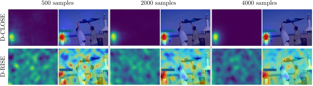
Since XAI methods can perform differently with varying number of samples nguyen2021evaluation, we compare D-CLOSE with D-RISE in different amounts of data (Fig. 9) to show that our method produces better results without being influenced by the number of generated samples. When evaluating both methods on large datasets, we use a fixed set of parameters for all objects in the image. We found out that D-RISE produced good results only by fine-tuning each parameter to fit each object’s geometry; otherwise, D-RISE’s saliency map is quite unfocused and provides weak localization in some cases. While D-CLOSE’s explanation is more stable with the number of samples generated, the noise in the saliency map decreases, and more focus is on the important regions in the image.
5.1.2 Object discrimination visualization
We conduct experiments to measure whether our proposed D-CLOSE has good object discrimination ability. As shown in Fig. 7, D-CLOSE’s explanations focus more on the object’s shape inside the bounding box. They often clearly distinguish the boundaries of objects, significantly when multiple objects are overlapped.
5.2 Quantitative
We apply various metrics to compare our method’s plausibility and faithfulness with other methods.
5.2.1 Plausibility Evaluation
We use two standard metrics to evaluate XAI’s plausibility: Sparsity gomez2022metrics and Energy-based pointing game (EBPG) wang2020score, based on human-annotated bounding boxes. In our evaluation, we only consider explanations for detected bounding boxes that best match the ground truths for each class to compute these metrics.
5.2.2 Faithfulness Evaluation
Faithfulness evaluation metrics, including Deletion, Insertion petsiuk2018rise and Over-all zhang2021group measure the explanation’s completeness and consistency for the model’s predictions. Deletion checks whether removing these important pixels severely degrades the model’s predictions for that object. For Insertion, it measures the increase in probability as more important pixels are included. Over-all score is the difference between Insertion and Deletion.
| Ablation Settings | Sparsity | EBPG (%) | Over-all (%) | ||
| Superpixel Segment | Density Map | Feature Fusion | |||
| ✓ | ✗ | ✗ | |||
| ✓ | ✓ | ✗ | |||
| ✓ | ✗ | ✓ | |||
| ✓ | ✓ | ✓ | 25.02 | 35.45 | 88.14 |
| Small | Middle | Large | Small+Middle+Large | |||||||||
|---|---|---|---|---|---|---|---|---|---|---|---|---|
| Metrics | Grad-CAM | D-RISE | D-CLOSE | Grad-CAM | D-RISE | D-CLOSE | Grad-CAM | D-RISE | D-CLOSE | Grad-CAM | D-RISE | D-CLOSE |
| Sparsity | 21.46 | 4.81 | 28.00 | 9.22 | 2.67 | 12.18 | 7.80 | 2.41 | 8.49 | 19.47 | 4.43 | 25.02 |
| EBPG (%) | 11.52 | 0.06 | 28.34 | 59.11 | 26.89 | 69.50 | 81.39 | 55.57 | 84.22 | 26.86 | 11.17 | 35.45 |
| Del (%) | 3.27 | 2.27 | 1.21 | 13.92 | 12.28 | 6.53 | 25.07 | 17.43 | 12.57 | 5.73 | 4.26 | 2.71 |
| Ins (%) | 71.13 | 83.27 | 92.35 | 68.78 | 73.06 | 85.74 | 62.03 | 64.05 | 78.92 | 70.18 | 81.19 | 90.85 |
| Over-all (%) | 67.86 | 81.00 | 91.14 | 54.86 | 60.78 | 79.21 | 36.96 | 46.62 | 66.35 | 64.45 | 76.93 | 88.14 |

| Method | D-RISE | D-CLOSE |
|---|---|---|
| Running time (s) | 98.67 | 70 |
5.3 Ablation studies
Our method proposes to combine three important components, including multi-scale superpixel segment, density normalization, and multi-scale feature fusion. We perform the experiments to investigate the contribution level of each part to the final explanation performance. The results are reported in Table 1.
Superpixel Segment. To validate the effectiveness of the superpixel segment step, we compare the evaluation metrics results using the superpixel segment results (row 1 of Table 1) and the D-RISE results (Table 2.) With this, we help increase 1.07% EBPG and 10.38% over-all score.
Density map. In the proposed D-CLOSE, we have introduced density map normalization, which can produce smoother and more object-focused saliency maps. From Table 1 (row 2), we can see that the density map can boost 3.01 sparsity, 2.93% EBPG, and 0.06% over-all score, compared to just adding superpixel segment step.
Multi-scale Feature Fusion. As shown in Table 1, we get impressive performance (21.09 sparsity, 22.03% EBPG, 0.79% over-all score) using multi-scale feature fusion. This result is comprehensible since this step removes the most noise and keeps only the most important features. Experiments also reflect that this step has the most significant influence on the final explanation. Finally, the amalgamation of the three aforementioned steps yields a result that is markedly superior to the outcome of implementing each step in isolation.
6 Results
As mentioned in Sec. 1, D-RISE is only effective when fine-tuning hyperparameters for individual objects. While our method can be applied to different sizes of objects with only one set of parameters for the entire dataset. To validate this, we first use 5000 images from the MS-COCO validation dataset lin2014microsoft and calculate the ratio of the bounding box size with the input image. We then use these ratios as input to the -means clustering algorithm na2010research to divide the objects into three groups corresponding to the objects belonging to small, middle, and large groups. We calculate quantitative metrics for each of these groups and for the entire data set to demonstrate the effectiveness of D-CLOSE. Based on the results in Table 2, we observe that D-CLOSE outperforms Grad-CAM and D-RISE on all quantitative metrics. To the best of our knowledge, our evaluation is the first to calculate quantitative metrics for distinct object groups. Besides, in Table 3, we also summarize the average inference time results for D-RISE and the proposed D-CLOSE. Our method is 1.4 times faster than D-RISE and achieves much better performance.
7 Conclusions
In this paper, we introduced D-CLOSE, a new XAI method that can explain the decisions of any object detector. Our method samples the input with multiple levels of segmentation to make the explanation more stable and smooth. We proposed using quantitative metrics for each object group to demonstrate that our approach performs better than previous state-of-the-art methods. We conducted in-depth analyzes of the model’s prediction errors and the implementation of D-CLOSE in real-world images. In future work, we want to optimize the computation time of XAI by removing redundant data samples during masking to debug and create workflows that improve model performance. Our code is available at https://github.com/Binh24399/D-CLOSE.
References
- (1) Radhakrishna Achanta, Appu Shaji, Kevin Smith, Aurelien Lucchi, Pascal Fua, and Sabine Süsstrunk. Slic superpixels. Technical report, 2010.
- (2) Julius Adebayo, Justin Gilmer, Michael Muelly, Ian Goodfellow, Moritz Hardt, and Been Kim. Sanity checks for saliency maps. Advances in neural information processing systems, 31, 2018.
- (3) Sebastian Bach, Alexander Binder, Grégoire Montavon, Frederick Klauschen, Klaus-Robert Müller, and Wojciech Samek. On pixel-wise explanations for non-linear classifier decisions by layer-wise relevance propagation. PloS one, 10(7):e0130140, 2015.
- (4) Jens Bayer, David Münch, and Michael Arens. A comparison of deep saliency map generators on multispectral data in object detection. In Counterterrorism, Crime Fighting, Forensics, and Surveillance Technologies V, volume 11869, pages 61–74. SPIE, 2021.
- (5) Aditya Chattopadhay, Anirban Sarkar, Prantik Howlader, and Vineeth N Balasubramanian. Grad-cam++: Generalized gradient-based visual explanations for deep convolutional networks. In 2018 IEEE winter conference on applications of computer vision (WACV), pages 839–847. IEEE, 2018.
- (6) Jessica Cooper, Ognjen Arandjelović, and David J Harrison. Believe the hipe: Hierarchical perturbation for fast, robust and model-agnostic explanations. arXiv preprint arXiv:2103.05108, 2021.
- (7) Arun Das and Paul Rad. Opportunities and challenges in explainable artificial intelligence (xai): A survey. arXiv preprint arXiv:2006.11371, 2020.
- (8) Truong-Dong Do, Minh-Thien Duong, Quoc-Vu Dang, and My-Ha Le. Real-time self-driving car navigation using deep neural network. In 2018 4th International Conference on Green Technology and Sustainable Development (GTSD), pages 7–12. IEEE, 2018.
- (9) Zheng Ge, Songtao Liu, Feng Wang, Zeming Li, and Jian Sun. Yolox: Exceeding yolo series in 2021. arXiv preprint arXiv:2107.08430, 2021.
- (10) Tristan Gomez, Thomas Fréour, and Harold Mouchère. Metrics for saliency map evaluation of deep learning explanation methods. In Pattern Recognition and Artificial Intelligence: Third International Conference, ICPRAI 2022, Paris, France, June 1–3, 2022, Proceedings, Part I, pages 84–95. Springer, 2022.
- (11) Denis Gudovskiy, Alec Hodgkinson, Takuya Yamaguchi, Yasunori Ishii, and Sotaro Tsukizawa. Explain to fix: A framework to interpret and correct dnn object detector predictions. arXiv preprint arXiv:1811.08011, 2018.
- (12) Thomas Hartley, Kirill Sidorov, Christopher Willis, and David Marshall. Swag: Superpixels weighted by average gradients for explanations of cnns. In Proceedings of the IEEE/CVF Winter Conference on Applications of Computer Vision, pages 423–432, 2021.
- (13) Derek Hoiem, Yodsawalai Chodpathumwan, and Qieyun Dai. Diagnosing error in object detectors. In European conference on computer vision, pages 340–353. Springer, 2012.
- (14) Andrei Kapishnikov, Tolga Bolukbasi, Fernanda Viégas, and Michael Terry. Xrai: Better attributions through regions. In Proceedings of the IEEE/CVF International Conference on Computer Vision, pages 4948–4957, 2019.
- (15) Tsung-Yi Lin, Michael Maire, Serge Belongie, James Hays, Pietro Perona, Deva Ramanan, Piotr Dollár, and C Lawrence Zitnick. Microsoft coco: Common objects in context. In European conference on computer vision, pages 740–755. Springer, 2014.
- (16) Wei Liu, Dragomir Anguelov, Dumitru Erhan, Christian Szegedy, Scott Reed, Cheng-Yang Fu, and Alexander C Berg. Ssd: Single shot multibox detector. In European conference on computer vision, pages 21–37. Springer, 2016.
- (17) Scott M Lundberg and Su-In Lee. A unified approach to interpreting model predictions. Advances in neural information processing systems, 30, 2017.
- (18) Riccardo Miotto, Fei Wang, Shuang Wang, Xiaoqian Jiang, and Joel T Dudley. Deep learning for healthcare: review, opportunities and challenges. Briefings in bioinformatics, 19(6):1236–1246, 2018.
- (19) Shi Na, Liu Xumin, and Guan Yong. Research on k-means clustering algorithm: An improved k-means clustering algorithm. In 2010 Third International Symposium on intelligent information technology and security informatics, pages 63–67. Ieee, 2010.
- (20) Hung Truong Thanh Nguyen, Hung Quoc Cao, Khang Vo Thanh Nguyen, and Nguyen Dinh Khoi Pham. Evaluation of explainable artificial intelligence: Shap, lime, and cam. In Proceedings of the FPT AI Conference, pages 1–6, 2021.
- (21) Phong X Nguyen, Hung Q Cao, Khang VT Nguyen, Hung Nguyen, and Takehisa Yairi. Secam: Tightly accelerate the image explanation via region-based segmentation. IEICE TRANSACTIONS on Information and Systems, 105(8):1401–1417, 2022.
- (22) Truong Thanh Hung Nguyen, Van Binh Truong, Vo Thanh Khang Nguyen, Quoc Hung Cao, and Quoc Khanh Nguyen. Towards trust of explainable ai in thyroid nodule diagnosis. arXiv preprint arXiv:2303.04731, 2023.
- (23) Nobuyuki Otsu. A threshold selection method from gray-level histograms. IEEE transactions on systems, man, and cybernetics, 9(1):62–66, 1979.
- (24) Vitali Petsiuk, Abir Das, and Kate Saenko. Rise: Randomized input sampling for explanation of black-box models. arXiv preprint arXiv:1806.07421, 2018.
- (25) Vitali Petsiuk, Rajiv Jain, Varun Manjunatha, Vlad I Morariu, Ashutosh Mehra, Vicente Ordonez, and Kate Saenko. Black-box explanation of object detectors via saliency maps. In Proceedings of the IEEE/CVF Conference on Computer Vision and Pattern Recognition, pages 11443–11452, 2021.
- (26) Joseph Redmon, Santosh Divvala, Ross Girshick, and Ali Farhadi. You only look once: Unified, real-time object detection. In Proceedings of the IEEE conference on computer vision and pattern recognition, pages 779–788, 2016.
- (27) General Data Protection Regulation. General data protection regulation (gdpr). Intersoft Consulting, Accessed in October, 24(1), 2018.
- (28) Shaoqing Ren, Kaiming He, Ross Girshick, and Jian Sun. Faster r-cnn: Towards real-time object detection with region proposal networks. Advances in neural information processing systems, 28, 2015.
- (29) Marco Tulio Ribeiro, Sameer Singh, and Carlos Guestrin. ” why should i trust you?” explaining the predictions of any classifier. In Proceedings of the 22nd ACM SIGKDD international conference on knowledge discovery and data mining, pages 1135–1144, 2016.
- (30) Jonas Herskind Sejr, Peter Schneider-Kamp, and Naeem Ayoub. Surrogate object detection explainer (sodex) with yolov4 and lime. Machine Learning and Knowledge Extraction, 3(3):662–671, 2021.
- (31) Ramprasaath R Selvaraju, Michael Cogswell, Abhishek Das, Ramakrishna Vedantam, Devi Parikh, and Dhruv Batra. Grad-cam: Visual explanations from deep networks via gradient-based localization. In Proceedings of the IEEE international conference on computer vision, pages 618–626, 2017.
- (32) Avanti Shrikumar, Peyton Greenside, and Anshul Kundaje. Learning important features through propagating activation differences. In International conference on machine learning, pages 3145–3153. PMLR, 2017.
- (33) Karen Simonyan, Andrea Vedaldi, and Andrew Zisserman. Visualising image classification models and saliency maps. Deep Inside Convolutional Networks, 2014.
- (34) Mahesh Sudhakar, Sam Sattarzadeh, Konstantinos N Plataniotis, Jongseong Jang, Yeonjeong Jeong, and Hyunwoo Kim. Ada-sise: adaptive semantic input sampling for efficient explanation of convolutional neural networks. In ICASSP 2021-2021 IEEE International Conference on Acoustics, Speech and Signal Processing (ICASSP), pages 1715–1719. IEEE, 2021.
- (35) Karasawa Takumi, Kohei Watanabe, Qishen Ha, Antonio Tejero-De-Pablos, Yoshitaka Ushiku, and Tatsuya Harada. Multispectral object detection for autonomous vehicles. In Proceedings of the on Thematic Workshops of ACM Multimedia 2017, pages 35–43, 2017.
- (36) Hideomi Tsunakawa, Yoshitaka Kameya, Hanju Lee, Yosuke Shinya, and Naoki Mitsumoto. Contrastive relevance propagation for interpreting predictions by a single-shot object detector. In 2019 International Joint Conference on Neural Networks (IJCNN), pages 1–9. IEEE, 2019.
- (37) Jorg Wagner, Jan Mathias Kohler, Tobias Gindele, Leon Hetzel, Jakob Thaddaus Wiedemer, and Sven Behnke. Interpretable and fine-grained visual explanations for convolutional neural networks. In Proceedings of the IEEE/CVF Conference on Computer Vision and Pattern Recognition, pages 9097–9107, 2019.
- (38) Haofan Wang, Zifan Wang, Mengnan Du, Fan Yang, Zijian Zhang, Sirui Ding, Piotr Mardziel, and Xia Hu. Score-cam: Score-weighted visual explanations for convolutional neural networks. In Proceedings of the IEEE/CVF conference on computer vision and pattern recognition workshops, pages 24–25, 2020.
- (39) Pengfei Xia, Hongjing Niu, Ziqiang Li, and Bin Li. On the receptive field misalignment in cam-based visual explanations. Pattern Recognition Letters, 152:275–282, 2021.
- (40) Qing Yang, Xia Zhu, Jong-Kae Fwu, Yun Ye, Ganmei You, and Yuan Zhu. Mfpp: Morphological fragmental perturbation pyramid for black-box model explanations. In 2020 25th International Conference on Pattern Recognition (ICPR), pages 1376–1383. IEEE, 2021.
- (41) Qinglong Zhang, Lu Rao, and Yubin Yang. Group-cam: group score-weighted visual explanations for deep convolutional networks. arXiv preprint arXiv:2103.13859, 2021.
- (42) Shifeng Zhang, Yiliang Xie, Jun Wan, Hansheng Xia, Stan Z Li, and Guodong Guo. Widerperson: A diverse dataset for dense pedestrian detection in the wild. IEEE Transactions on Multimedia, 22(2):380–393, 2019.
- (43) Bolei Zhou, Aditya Khosla, Agata Lapedriza, Aude Oliva, and Antonio Torralba. Learning deep features for discriminative localization. In Proceedings of the IEEE conference on computer vision and pattern recognition, pages 2921–2929, 2016.
- (44) Zhengxia Zou, Zhenwei Shi, Yuhong Guo, and Jieping Ye. Object detection in 20 years: A survey. arXiv preprint arXiv:1905.05055, 2019.