On Emergence of Clean-Priority Learning in Early Stopped Neural Networks
Abstract
When random label noise is added to a training dataset, the prediction error of a neural network on a label-noise-free test dataset initially improves during early training but eventually deteriorates, following a U-shaped dependence on training time. This behaviour is believed to be a result of neural networks learning the pattern of clean data first and fitting the noise later in the training, a phenomenon that we refer to as clean-priority learning. In this study, we aim to explore the learning dynamics underlying this phenomenon. We theoretically demonstrate that, in the early stage of training, the update direction of gradient descent is determined by the clean subset of training data, leaving the noisy subset has minimal to no impact, resulting in a prioritization of clean learning. Moreover, we show both theoretically and experimentally, as the clean-priority learning goes on, the dominance of the gradients of clean samples over those of noisy samples diminishes, and finally results in a termination of the clean-priority learning and fitting of the noisy samples.
Keywords:
Early stopping, dynamics, label noisy1 Introduction
Recent studies suggest that Neural Network (NN) models tend to first learn the patterns in the clean data and overfit the noise at a later stage (Arpit et al. 2017; Li et al. 2020). We refer to this phenomena as clean-priority learning. Real datasets may have intrinsic label noise, which is why early stopping can be useful in practice, saving a significant amount of unnecessary computation cost.
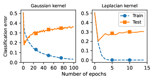
To study clean-priority learning phenomena, we intentionally add label noise to the training data set and leave the test data set untouched, this is a common setting in literature (see, for example, (Zhang et al. 2021; Nakkiran et al. 2021; Belkin et al. 2018)). Figure 1 illustrate this for a MNIST classification task using CNN. The test prediction error exhibits a U-shaped dependence on training time, with an initial decrease followed by an increase after the early stopping point. The observation is that in the intermediate steps, especially around the early stopping point, the test performance can be significantly better than the label noise level added to the training set (below the dashed line).

To further explore this phenomenon, we address the following fundamental questions:
- 1.
What is the underlying mechanism by which neural networks learn the clean data first and fit the noise in later stages?
- 2.
How does the model performance deteriorate after the early stopping point ?
At the outset, we analyze the configuration of sample-wise gradients (or its variant, for multi-class classification) on the training dataset, at the neural network initialization. Our objective is to examine whether there exists any pattern among the gradients that can explain the clean-priority learning phenomenon. Our analysis reveals that, at initialization, samples within the same class (before label corruption), which are presumably more similar to each other, tend to have their sample-wise gradients relatively closer in vector directions (compared to the samples from different classes). The label corruption, which flips the label to a different class, flips the corresponding sample-wise gradient to its opposite direction. Consequently, the sum of the noisy sample gradients is in sharp opposite direction of that of the clean sample gradients.
The key observation is that, due to the dominance of the population of the clean samples, in the early stage of learning, the gradient of noisy subset is cancelled out, and essentially makes no contribution on the gradient descent (GD) update direction11 1 To be more precise, the only effect of the noisy subset gradient is resulting in a smaller GD step size.. It is also worth noting that almost all clean sample-wise gradient vectors “agree” with the GD update (i.e., have positive projection), while almost all noisy sample-wise gradients are “against” the GD update. As a result, the individual loss on each clean sample is decreased, and that on each noisy sample is increased. Hence, we see that, in the early stage, the GD algorithm is determined by the clean samples and exhibits the clean-priority learning.
We further show that as the clean-priority learning process continues, the clean subset gradient’s dominance over the noisy subset gradually diminishes. This is particularly evident around the early stopping point, at which the noisy subset gradient begins to make a meaningful contribution, causing the model to fit the noisy samples along with the clean ones. This new trend in learning behavior is expected to hurt the model’s performance, which was previously based primarily on the clean samples.
In summary, we make the following contributions:
- •
learning dynamics. In the early stage of learning of neural networks, the noisy samples contribution to the GD update is cancelled out by that of the clean samples, which is the key mechanism underlying clean-priority learning. However, this clean-priority learning behavior gradually fades as the dominance of the clean subset diminishes, particularly around the early stopping point. We experimentally verify our findings on deep neural networks on various classification problems.
- •
For fully connected networks with mild assumption on data we theoretically prove our empirical observation.
- •
In addition, we find for neural networks, at initialization, sample-wise gradients from the same class tend to have relatively similar directions, when there is no label noise.
The paper is organized as follows: in Section 2, we describe the setup of the problems and introduce necessary concepts and notations. In Section 3, we analyze the sample-wise gradients at initialization of neural network, for binary classification. In Section 4, we show the learning dynamics, especially the clean-priority learning, on binary classification. In Section 5, we extend our study and findings to multi-class classification problems.
1.1 Related works
Early stopping is often considered as a regularization technique and is widely used in practice to obtain good performance for machine learning models (Zhang & Wallace 2017; Gal & Ghahramani 2016; Graves et al. 2013). Early stopping also received a lot theoretical analyses, both on non-neural network models, especially linear regression and kernel regression (Yao et al. 2007; Ali et al. 2019; Xu et al. 2022; Shen et al. 2022), and on neural networks (Zhang et al. 2021; Ji et al. 2021).
Recent studies suggest that, when random label noise presents, neural networks fit the clean data first and “overfit” the noise later on (Arpit et al. 2017; Li et al. 2020; Bai et al. 2021). For example, based on experimental observations that maximum validation set accuracy is achieved before good training set accuracy, the work (Arpit et al. 2017) conjectures that the neural network learns clean patterns first. However, there is no explanation on why and how the clean-priority learning happens. In another work (Li et al. 2020), assuming (almost) perfectly cluster-able data and uniform conditioning on Jacobian matrices, proves that clean data are fit by two-layer neural networks in an early stage. However, this data assumption requires, at the same location of each noisy sample, there must exist several (at least , with being the label noise level) clean samples. This assumption is often not met by actual datasets.
To the best of our knowledge, our work is the first to elucidate the mechanism underlying the clean-priority phenomenon, offering a fresh perspective on its dynamics.
2 Problem setup and preliminary
In this paper, we consider supervised classification problems.
Datasets.
There is a training dataset of size . In each sample , there are input features and a label . For binary (-class) classification problems, the label is binary; for multi-class classification problems, the label is one-hot encoded, , where is the total number of classes. We further denote , , as the subset of that is composed of samples from the -th class. It is easy to see, .
We assume the labels in are randomly corrupted. Specifically, if denote as the ground truth label of , there exists a non-empty set
| (1) |
Furthermore, the labels in is uniformly randomly distributed across all the class labels except . We call as the noisy subset and its elements as noisy samples. We also define the clean subset as the compliment, i.e., , and call its elements as clean samples. The noise level is defined as the ratio . In this paper, we set , i.e., the majority of training samples are not corrupted. We also denote as the ground-truth-labeled dataset: .
In addition, there is a test dataset which is i.i.d. drawn from the same data distribution as the training set , except that the labels of test set are not corrupted.
Optimization.
Given an arbitrary dataset and a model which is parameterized by and takes an input , we define the loss function as
| (2) |
with is evaluated on a single sample and is a function of the model output and label . We use the logistic loss for binary classification problems, and the cross entropy loss for multi-class problems. In this paper, we use neural networks as the model. In case of binary classification problems, the output layer of has only one neuron, and there exists a sigmoid function on top such that the output . In case of multi-class classification problems, the neural network has output neurons, and there exists a softmax function to normalize the outputs. Throughout the paper, we assume that the neural network is large enough so that the training data can be exactly fit. This is usually satisfied when the neural network is over-parameterized (Liu et al. 2022a).
The optimization goal is to minimize the empirical loss function (i.e., loss function on the training dataset ):
| (3) |
The above loss function is usually optimized by gradient descent (or its stochastic variants) which has the following update form:
| (4) | ||||
Here, is the gradient of loss w.r.t. the neural network parameters .
Sample-wise gradients.
We call sample-wise gradient, as it is evaluated on a single sample, and denote it as for short. As there are samples in , at each point in the parameter space, we have sample-wise gradients, each of which is of dimension .
Denote as the pre-activation output neuron(s) before activation, which is in for binary classification, and is in for multi-class classification. The sample-wise gradient for a given sample has the following form (Bishop & Nasrabadi 2006):
| (5) |
Note that the above expression is a scalar-vector multiplication for binary classification, and is a vector-matrix multiplication for multi-class classification.
We note that the sample-wise gradient will be one of our major quantities, and play a fundamental role in the analysis through out this paper.
3 Sample-wise gradients at initialization for binary classification
In this section, we analyze the configuration of the sample-wise gradients at randomly initialization of neural networks for binary classification.
We start with the expression Eq.(5) of the sample-wise gradient . For binary classification, is proportional to the model derivative , up to a scalar factor . In Section 3.1, we focus on the directions of , which is label independent. Then, in Section 3.2, we discuss the effects of the label-related factor and label noise on the direction of sample-wise gradients.
3.1 Direction of the model derivative
Given any two inputs , we denote the angle between and in the data space by , and denote the angle between the two vectors and by . In this subsection, we are concerned with the connection between and at the network initialization.
Consider the following two types of neural networks: a two-layer linear network , which is defined as
| (6) |
and a two-layer ReLU network , which is defined as
| (7) |
Here, is the element-wise ReLU activation function, and are the first layer and second layer parameters, respectively. We denoted as the collection of all the parameters. We use the NTK parameterization (Jacot et al. 2018) for the networks; namely, each parameter is i.i.d. initialized using the normal distribution and there exist a scaling factor explicitly on each hidden layer.

The following theorem and its corollary show the relation between and . (Proofs in Appendix A.1).
Theorem 3.1.
Corollary 3.2.
Consider the same networks and as in Theorem 3.1. For both networks, the following holds: for any inputs , and , if , then , for .
The theorem and corollary suggest that: similar inputs (small angle ) induce similar model derivatives (small angle ).
Remark 3.3 (Not just at initialization).
As discussed in (Liu et al. 2020; Liu et al. 2022b), the model derivative is constant during optimization for infinitely wide neural networks. Hence, the angle between model derivatives is also constant, and Theorem 3.1 and Corollary 3.2 apply to any time stamp of the network training.
Experimental verification.
We experimentally verify the above theoretical results on neural networks with large width. Specifically, we consider six neural networks: three linear networks with , and layers, respectively; and three ReLU networks with , and layers. Each hidden layer of each neural network has neurons. For each network, we compute the model derivatives on the -sphere , at the network initialization. Figure 2 shows the relations between the angle and .22 2 The curves for the three linear networks are almost identical and not visually distinguishable, we only present the one for -layer linear network in Figure 2. We observe that the curves for the -layer networks match Theorem 3.1. More importantly, the experiments suggest that the same or similar relations, as well as Corollary 3.2, still hold for deep neural networks, although our analysis is conducted on shallow networks.
Consider the following synthetic dataset (also shown in the left panel of Figure 3): two separated data clusters in a -dimensional space. We use a -layer ReLU network of width at its initialization to compute the sample-wise model derivatives . The right panel of Figure 3 shows the distributions of angle for data pairs from the same cluster (“within”) and from different clusters (“between”). It can be easily seen that the “within” distribution has smaller angles than the “between” distribution, which is expected as the data from the same clusters are more similar.

3.2 Directions of the sample-wise gradients
Now, we consider the sample-wise gradients at initialization, using Eq.(5). We note that the direction of is determined by and the label . This is because only the sign (not the magnitude) of may affect the direction, and the post-activation output is always in and label is either or .
Motivated by this observation, for a fixed class , we consider the following subsets: clean subset , noisy subset , and . We note that and have the same input distribution but different labels , while and have the same labels but different input distributions.
For these subsets, we denote their corresponding sets of sample-wise gradients as , and , respectively. We also define the corresponding subset gradients as the sum of all sample-wise gradients in the subset: , for . the direction of is the same as that of the average gradient in the subset.
Direction of sample-wise gradients. We consider the angles between sample-wise gradients, and denote by .
First we consider the clean subset. Within , the factor always have the same sign, as the label is the same. Thus, the directional distribution of is identical to the distribution, which has been analyzed in Section 3.1. Presumably, inputs from the same ground truth class tend to be more similar (with small angles ), compared to others. Applying Corollary 3.2, we expect the angles , and therefore also, within this subset are relatively small. The green plots of Figure 4 show numerical verification of the distributions for the clean subset .33 3 For illustration purpose, we compare each sample-wise gradient with the average direction, represented by . We see that tends to concentrate around relatively small angles.
The interesting part is about the noisy subset . This subset shares the same input distribution, hence distribution as well, with the clean subset. However, due to different label , the factor has different sign from that of clean samples, which flips all to the opposite direction of those in . As a consequence, sample-wise gradients between and makes large angles ; and the noisy subset gradient is sharply opposite to . Figure 4 experimentally verifies this phenomenon. The red histograms, representing the distribution for noisy subset, are symmetric to the green ones and locate at large angles. The red dash lines representing the angle between and is almost close to .
Lastly, the subset , having different ground truth labels with the other two subsets, has different input distributions. By Corollary 3.2, the sample-wise gradients of this subset are expected to be not align with those of the other two subsets (as shown by the blue histograms in Figure 4). Moreover, the subset gradient should have a significant component orthogonal to and (as shown by the blue dash lines in Figure 4).
Magnitudes of subset gradients. We are interested in the magnitudes of and . By definition, for ,
where the expectation is taken over the corresponding data subset. We know that is the same for clean and noisy subsets. In addition, are opposite for these two subsets, as is by random guess and for one subset and for the other. Hence, we see that the magnitudes are determined by the subset population, and we have
| (8) |

4 Learning dynamics of binary classification
In this section, we analyze the learning dynamics of binary classification with label noise in the training dataset.
Specifically, we show that in the early stage of training, the dynamics exhibits a clean-priority learning characteristic, due to a dominance of the clean subset in first-order information, i.e., sample-wise gradients. We further show that in later stage of training, this dominance fades away and clean-priority learning terminates, resulting in a fitting of the noisy samples and worsening of the test performance.
We partition the optimization procedure into two stages: early stage which happens before the early stopping point; and later stage which is after the early stopping point.

4.1 Initialization & early stage
In Section 3, we have seen that, at initialization,
| (9) |
with . We note that, during training, the model derivative for a wide neural network is found to barely change (Liu et al. 2020):
By Eq.(5), this implies that each sample-wise gradient keeps its direction unchanged during training (but changes in magnitude through the factor ). Therefore, we make the following assumption:
Assumption 4.1.
There exist a time and a sequence , with each , such that, for all and , the following holds .
Define as the summation of the sample-wise gradients with ground truth labels, i.e., . By the assumption, we have for all and ,
| (10) |
On the other hand, by definition, we have for full gradient
| (11) |
Combining Assumption 4.1 and Eqs.(10) and (11), we get that the full gradient on the training data has the same direction with that on the ground-truth-labeled data . Hence, we have the following proposition.
Proposition 4.2 (Update rules).
Remark 4.3 (mini-batch scenario).
In mini-batch SGD, similar relation of Eq.(12) also holds for a mini-batch estimation , as long as the sampling of the mini-batch is independent of the label noise and the batch size is not too small such that the majority of samples are clean in the batches. Hence, in the following, we do not explicitly write out the dependence on the mini-batches.
The theorem states that, after adding label noise to the training dataset, the gradient descent update is equivalent to the one without label noise (except a different learning rate ). In another word, the gradient descent does not essentially “see” the noisy data and its update direction is determined only by the clean samples.
Clean-priority learning.
This theorem implies the following learning characteristics of what we call clean-priority learning, as we described below.
Training loss and accuracy on subsets. The loss on the clean subset keeps decreasing, while the loss on the noisy subset is increasing, as formally stated in the following Theorem (see the proof in Appendix A.4):
Theorem 4.4.
Suppose Assumption 4.1 holds with time and sequence , . We have, for all and sufficiently small ,
Accordingly, the training accuracy on the clean subset is increased, and that on the noisy subset is decreased.
Residual magnitude: . As a consequence of the decreasing clean subset loss , the clean training samples are learned, in the sense that the network output moves towards its corresponding label , i.e., decreases on the clean subset. On the other hand, the increase of the results in that, on the noisy subset, the network output moves away from its corresponding label , but towards its ground truth label . Namely, the noisy subset is not learnt.
Test loss. As the test dataset is not label-corrupted and is drawn from the same data distribution as , it is expected that the update rule in Eq.(12) decreases the test loss .
Figure 5 shows the clean-priority learning phenomenon on a binary classification of two classes of MNIST. The relevant part is the early stage, i.e., before the early stopping point (left of the vertical dash line). As one can see, in this stage, the prediction error and noisy subset loss keep increasing (See Appendix B for subset loss curves). Especially, the prediction error increases from a random guess (error ) at initialization towards . Meanwhile, the clean subset loss and prediction error keep decreasing. Moreover, the average residual magnitude decreases on the clean subset, but increases on the noisy subset, implying that only clean subset is learnt. These behaviors illustrate that in the early stage the learning dynamics prioritize the clean samples.
In short, in the early stage, the clean-priority learning prioritizes the learning on clean training samples. The interesting point is that, although it seems impossible to distinguish the clean from the noisy directly from the data, this prioritization is possible because the model have access to the first-order information, i.e., sample-wise gradients. Importantly, it is this awareness of the clean samples and this prioritization in the early stage that allow the possibility of achieving test performances better than the noisy level.
4.2 Early stopping point & later stage
As we have seen in the above subsection, the dominance of the magnitude over is one of the key reasons to maintain the clean-priority learning in the early stage. However, we shall see shortly that this dominance diminish as the training goes on, resulting in a final termination of the clean-priority learning.
Diminishing dominance of the clean gradient.
Recall that the sample-wise gradient is proportional to the magnitude of the residual: The learning of a sample, i.e., decreased , results in a decrease in the magnitude . As an effect of the clean-priority learning, the residuals magnitude evolves differently for different data subsets: decreases on the clean subset , but increases on the noisy subset . This difference leads to the diminishment of the dominance of clean subset , which originates from the dominance of the population of clean training samples.
Theorem 4.5 (Diminishing dominance of the clean gradient).
Assume the neural network is infinitely wide and the learning rate of the gradient descent is sufficiently small. Suppose Assumption 4.1 holds with time and sequence . The sequence monotonically increases: for all , .
Please find the proof in Appendix A.5. As measures this clean dominance ( close to means less dominant), this theorem indicates that the dominance diminishes as the training goes on.
Figure 6 illustrates this diminishing dominance on the two class MNIST classification problem. In the early stage, the ratio starts with a value around the ratio of population , and monotonically decrease to around at or before the early stopping point, indicating that the dominance vanishes.


Learning the noisy samples.
In the later stage (i.e., after the early stopping point), the magnitudes of and are similar, and there is no apparent dominance of one over the other. Then, the model and algorithm do not distinguish the clean subset from the noisy one, and there will be no clean-priority learning. In this stage, the model learns both the clean and noisy subsets, aiming at achieving exact fitting of the training data. Ultimately, training errors of both subsets converge to zero.
It is expected that in this stage the loss and prediction error on the test dataset become worse, as the learning on the noisy subset contaminates the performance achieved by the clean-priority learning in the earlier stage.
As illustrated in Figure 5, after the early stopping point, the noisy subset starts to be learnt. Specifically, both training loss and error on this subset turn to decrease towards zero; the average residual magnitude turn to decrease, indicating that the network output is learnt to move towards its (corrupted) label. It is worth to note that the learning on the clean subset is still ongoing, as both training loss and error on this subset keeps decreasing.
In high level, before the first stage, the learning procedure prioritizes the clean training samples, allowing the superior-noise-level performance on the test dataset; in later stage, the learning procedure picks up the noisy samples, worsening the test performance toward the noise-level.
5 Multi-class classification
In this section we show that multi-class classification problems exhibit the same learning dynamics, especially the clean-priority learning, as described in Section 4.
For multi-class classification, we consider a variant of the sample-wise gradient, single-logit sample-wise gradient.
Single-logit sample-wise gradients.
In a -class classification problem, the neural network has output logits, and the labels are a -dimensional one-hot encoded vectors. One can view the neural network as co-existing binary classifiers. Specifically, for each , the -th logit is a binary classifier, and the -th component of the label is the binary label for .
By Eq.(5), the sample-wise gradient can be written as where
| (13) |
is the single-logit sample-wise gradient, which only depends on quantities of the corresponding single logit.
We point out that, the cleanness of a sample is only well defined with respect to each single logit, but not to the whole output. For example, consider a sample with ground truth label but is incorrectly labeled as class . For all the rest binary classifiers, except the -th and -st, this sample is always considered as the negative class, as for all or ; hence, the noisy sample is considered “clean”, for these binary classifiers. Therefore, a noisy sample is not necessarily noisy for all the binary classifiers.
With this observation, we consider the single-logit sample-wise gradient instead.
At initialization.
Given , the -logit sub-network (before softmax) is the same as the network discussed in Section 3, and the output . Hence, all the directional analysis for binary case (Section 3) still applies to the single-logit sample-wise gradient . See Appendix C for numerical verification.
Different from the sigmoid output activation which tends to predict an average of before training, the softmax has an average output around with random guess at initialization. This leads to when , and when . Recalling that and (hence the corresponding ) have the same distribution, using Eq.(13) we have
| (14a) | ||||
| (14b) | ||||
Therefore, we have the dominance of over at initialization, with a ratio

Learning dynamics.
As the configuration of is similar to that of a binary classification, we expect similar learning dynamics as discussed in Section 4, especially the clean-priority learning, happen for multi-class classification.
We conduct experiments to classify the MNIST (with added label noise ) and CIFAR-10 (with added label noise ) datasets using a CNN and a ResNet, respectively. As is shown in Figure 8 and Figure 7, in most of the early stage, the clean subset has clean dominance over the noise subset and the dynamics shows the clean-priority learning characteristic, decreasing the clean subset error and residual, but increasing the noisy subset error and residual. Furthermore, the dominance of the clean subset monotonically decreases (Figure 8) until the early stopping point. In the later stage, the networks start to learn the noisy subsets. See the detailed experimental setup in Appendix B.
6 Discussion and Future work
In this section, we aim to provide some insights into the relationship between the clean-priority phenomena described in this paper and previous works, as well as how this phenomena may manifest in other gradient descent-based learning algorithms.
Firstly, previous studies observed that, for certain very large models, the test classification error may exhibit a second descent in the later stages of training (Nakkiran et al. 2021). In such scenarios, our analysis still holds for the first descent and the subsequent ascent that follows it. Regarding the second descent, we hypothesize that it may be connected to certain types of underlying feature learning dynamics, for example, the Expected Gradient Outer Product (EGOP) (Radhakrishnan et al. 2022). However, further investigation is needed to confirm this hypothesis, and we leave it as a topic for future research.
Secondly, as can be seen in Figure 1, 5, and 7, This occurs sometime after the early stopping point. It suggests that while the model is fitting the noise, the test performance at convergence is not catastrophic, and still outperforms the random guess. This, in turn, implies that neural networks demonstrate a tempered over-fitting behavior, as described in (Mallinar et al. 2022).
Acknowledgments
We are grateful for the support from the National Science Foundation (NSF) and the Simons Foundation for the Collaboration on the Theoretical Foundations of Deep Learning (https://deepfoundations.ai/) through awards DMS-2031883 and #814639 and the TILOS institute (NSF CCF-2112665). This work used NVIDIA V100 GPUs NVLINK and HDR IB (Expanse GPU) at SDSC Dell Cluster through allocation TG-CIS220009 and also, Delta system at the National Center for Supercomputing Applications through allocation bbjr-delta-gpu from the Advanced Cyberinfrastructure Coordination Ecosystem: Services & Support (ACCESS) program, which is supported by National Science Foundation grants #2138259, #2138286, #2138307, #2137603, and #2138296.
References
- Ali et al. (2019) Ali, A., Kolter, J. Z., and Tibshirani, R. J. A continuous-time view of early stopping for least squares regression. In The 22nd international conference on artificial intelligence and statistics, pp. 1370–1378. PMLR, 2019.
- Arpit et al. (2017) Arpit, D., Jastrzebski, S., Ballas, N., Krueger, D., Bengio, E., Kanwal, M. S., Maharaj, T., Fischer, A., Courville, A., Bengio, Y., et al. A closer look at memorization in deep networks. In International conference on machine learning, pp. 233–242. PMLR, 2017.
- Bai et al. (2021) Bai, Y., Yang, E., Han, B., Yang, Y., Li, J., Mao, Y., Niu, G., and Liu, T. Understanding and improving early stopping for learning with noisy labels. Advances in Neural Information Processing Systems, 34:24392–24403, 2021.
- Belkin et al. (2018) Belkin, M., Ma, S., and Mandal, S. To understand deep learning we need to understand kernel learning. In International Conference on Machine Learning, pp. 541–549. PMLR, 2018.
- Bishop & Nasrabadi (2006) Bishop, C. M. and Nasrabadi, N. M. Pattern recognition and machine learning, volume 4. Springer, 2006.
- Gal & Ghahramani (2016) Gal, Y. and Ghahramani, Z. A theoretically grounded application of dropout in recurrent neural networks. Advances in neural information processing systems, 29, 2016.
- Graves et al. (2013) Graves, A., Mohamed, A.-r., and Hinton, G. Speech recognition with deep recurrent neural networks. In 2013 IEEE international conference on acoustics, speech and signal processing, pp. 6645–6649. Ieee, 2013.
- Jacot et al. (2018) Jacot, A., Gabriel, F., and Hongler, C. Neural tangent kernel: Convergence and generalization in neural networks. Advances in neural information processing systems, 31, 2018.
- Ji et al. (2021) Ji, Z., Li, J., and Telgarsky, M. Early-stopped neural networks are consistent. Advances in Neural Information Processing Systems, 34:1805–1817, 2021.
- Li et al. (2020) Li, M., Soltanolkotabi, M., and Oymak, S. Gradient descent with early stopping is provably robust to label noise for overparameterized neural networks. In International conference on artificial intelligence and statistics, pp. 4313–4324. PMLR, 2020.
- Liu et al. (2020) Liu, C., Zhu, L., and Belkin, M. On the linearity of large non-linear models: when and why the tangent kernel is constant. Advances in Neural Information Processing Systems, 33:15954–15964, 2020.
- Liu et al. (2022a) Liu, C., Zhu, L., and Belkin, M. Loss landscapes and optimization in over-parameterized non-linear systems and neural networks. Applied and Computational Harmonic Analysis, 59:85–116, 2022a.
- Liu et al. (2022b) Liu, C., Zhu, L., and Belkin, M. Transition to linearity of wide neural networks is an emerging property of assembling weak models. In International Conference on Learning Representations, 2022b.
- Mallinar et al. (2022) Mallinar, N. R., Simon, J. B., Abedsoltan, A., Pandit, P., Belkin, M., and Nakkiran, P. Benign, tempered, or catastrophic: Toward a refined taxonomy of overfitting. Advances in Neural Information Processing Systems, 2022.
- Nakkiran et al. (2021) Nakkiran, P., Kaplun, G., Bansal, Y., Yang, T., Barak, B., and Sutskever, I. Deep double descent: Where bigger models and more data hurt. Journal of Statistical Mechanics: Theory and Experiment, 2021(12):124003, 2021.
- Radhakrishnan et al. (2022) Radhakrishnan, A., Beaglehole, D., Pandit, P., and Belkin, M. Feature learning in neural networks and kernel machines that recursively learn features. arXiv preprint arXiv:2212.13881, 2022.
- Shen et al. (2022) Shen, R., Gao, L., and Ma, Y. On optimal early stopping: Over-informative versus under-informative parametrization. arXiv preprint arXiv:2202.09885, 2022.
- Xu et al. (2022) Xu, J., Teng, J., and Yao, A. C.-C. Relaxing the feature covariance assumption: Time-variant bounds for benign overfitting in linear regression. arXiv preprint arXiv:2202.06054, 2022.
- Yao et al. (2007) Yao, Y., Rosasco, L., and Caponnetto, A. On early stopping in gradient descent learning. Constructive Approximation, 26(2):289–315, 2007.
- Zhang et al. (2021) Zhang, C., Bengio, S., Hardt, M., Recht, B., and Vinyals, O. Understanding deep learning (still) requires rethinking generalization. Communications of the ACM, 64(3):107–115, 2021.
- Zhang & Wallace (2017) Zhang, Y. and Wallace, B. C. A sensitivity analysis of (and practitioners’ guide to) convolutional neural networks for sentence classification. In Proceedings of the Eighth International Joint Conference on Natural Language Processing (Volume 1: Long Papers), pp. 253–263, 2017.
- Zhu et al. (2022) Zhu, L., Liu, C., and Belkin, M. Transition to linearity of general neural networks with directed acyclic graph architecture. Advances in Neural Information Processing Systems, 35:5363–5375, 2022.
Appendix A Technical proofs
A.1 Proof of Theorem 3.1
We restate Theorem 3.1 below for easier reference.
Theorem A.1 (Theorem 3.1).
Proof.
We prove for the two neural networks separately.
Two-layer linear network . According to the definition of (Eq.(6)), its model derivative (at initialization with input ) can be written as
| (17) |
Here, and are the initialization instance of the parameters and , respectively.
Hence, for the two inputs and , the inner product
| (18) |
When the network width is infinite, we have the following lemma (see proof in Appendix A.3).
Lemma A.2.
Consider a matrix , with each entry of is i.i.d. drawn from . In the limit of ,
| (19) |
Using this lemma, we have in the limit of ,
| (20) |
Therefore,
Two-layer ReLU network . According to the definition of (Eq.(7)), its model derivative (at initialization with input ) can be written as
| (21) |
where is the (element-wise) indicator function.
For any two inputs and , the inner product
where is the -th row of the matrix , and is the -th component of the vector . In the limit of infinite width , this inner product converges to
As the vector is isotropically distributed and only appears in inner products with and , we can assume without loss of generality that (without ambiguity, we write as , and as , for short):
| (22) |
In this setting, the only relevant parts of are its first two components and . We write .
With Eq.(22), for the term , we have
In the equality above, we applied trigonometric subtraction formula for and , as well as the double angle formulas.
For the term , we have
Combining and , we have
| (23) |
Therefore,
| (24) |
Therefore, we conclude the proof of the theorem. ∎
A.2 Proof of Corollary 3.2
We restate Corollary 3.2 below.
Corollary A.3 (Corollary 3.2).
Consider the same networks and as in Theorem 3.1. For both networks, the following holds:
- 1.
given two inputs and , if , then ;
- 2.
for any three inputs , and , if , then .
Proof.
For the infinitely wide two-layer linear network , we have seen in Theorem 3.1 that
| (25) |
Hence, the corollary is trivial for .
Below, we consider the infinitely wide two-layer ReLU network . By Theorem 3.1, we have the connection
| (26) |
If , then using Taylor expansion on the right hand side, we have
Hence, , which implies . We conclude the first statement.
For the second statement of the corollary, note that when is in the right hand side (R.H.S.) of Eq.(26) is always positive, resulting in . For the rest of the statement, it suffices to prove the monotonicity of the relation in . This is done by having the monotonicity of the functions of and R.H.S.. To see the latter, we write
| (27) |
which is always non-positive in . Hence, we are done with the second statement. ∎
A.3 Proof of Lemma A.2
Proof.
We denote as the -th entry of the matrix . Therefore, . First we find the mean of each . Since are i.i.d. and has zero mean, we can easily see that for any index ,
Consequently,
That is .
Now we consider the variance of each . If we can explicitly write,
In the case of , then,
| (28) |
In the equality (a) above, we used the fact that . Therefore, .
Now applying Chebyshev’s inequality we get,
| (29) |
Obviously for any as , the R.H.S. goes to zero. Thus, ∎
A.4 Proof of Theorem 4.4
Proof.
First, note that the clean data has the same distribution as the noiseless (ground-truth-labelled) data. Hence, . By Proposition 4.2, the gradient descent minimizes , as long as the learning rate is small enough to avoid over-shooting. Therefore, it is straightforward to get that the gradient descent also decreases the clean subset loss .
A.5 Proof of Theorem 4.5
Proof.
First note that an infinitely wide feedforward neural network (before the activation function on output layer) is linear in its parameters, and can be written as (Liu et al. 2020; Zhu et al. 2022):
| (31) |
where is constant during training. As is known, the logistic regression loss (for an arbitrary ) on a linear model
| (32) |
is a convex function with respect to the parameters , where . Hence, at any point we have the Hessian matrix of the logistic regression loss is positive definite.
Now, consider the point with a sufficiently small step size . Using Assumption 4.1 and Eq.(11), we can also write as
For , we have
| (33) |
with being some point between and . Then,
By the convexity of the loss function (i.e., the positive definiteness of Hessian ), we easily get
Similarly for ,
Hence, for small , we get
Noting that
we obtain
| (34) |
Therefore, we conclude the proof of the theorem. ∎
The high-level idea of the above proof is that: (locally) decreasing a convex function along the opposite gradient direction, , results in shrinking the magnitude of the gradient; (locally) increasing a convex function along the gradient direction results in magnifying the gradient magnitude.
Appendix B Experimental setup details
Binary classification on two class of MNIST.
We extract two classes, the images with digits “7” and “9”, out from the MNIST datasets, and injected random label noise into each class in the training dataset (i.e., labels of randomly selected samples are flipped to the other class), leaving test set intact. We employ a fully connected neural network with 2 hidden layers, each containing 512 units and using the ReLU activation function, of the classification task. We use mini-batch SGD with batch size 256 to train this network.
Multi-class classification on MNIST.
We use the following CNN to classify the classes of MNIST. Specifically, this CNN contains two consecutive convolutional layers, with and channels, respectively. Both convolutional layers uses kernel size and are with stride . On top of the convolutional layers, there is one max pooling layer, followed by two fully connected layers with width 64 and 10, respectively.
We injected random label noise into each class of MNIST training set. We use mini-batch SGD with batch size 512 to training the neural network.
Multi-class classification on CIFAR-10.
For the CIFAR-10 dataset, we use a standard -layer ResNet (ResNet-9) to classify 44 4 For the detailed architecture, we use the implementation in https://github.com/cbenitez81/Resnet9/blob/main/model_rn.py.. We injected random label noise into each class of CIFAR-10 training set. We use mini-batch SGD with batch size 512 to training the neural network.
Appendix C Additional experimental results
C.1 Angle distribution for multi-class classification
We experimentally verify the directional distributions of single-logit sample-wise gradients on MNIST dataset. We use the same CNN as in Figure 7, and evaluate the angle distributions at the network initialization. Specifically, given , we consider the -th output logit. Note that, according to the one-hot encoding, only class has label and all the rest classes have label on this logit. Hence, the binary classifier at logit is essentially a one-versus-rest classifier. For each of these binary classifiers, we look at the angle distributions of the corresponding single-logit sample-wise gradients.
As shown in Figure 10, each sub-plot corresponds to one logit. We can see that, for each :
- •
The clean subset of class (green) has its single-logit sample-wise gradients concentrated at small angles .
- •
The noisy subset of class (red) has its single-logit sample-wise gradients in the opposite direction of clean ones, concentrating at large angles and being symmetric to the clean subset. The noisy subset gradient (red dash line) is sharply opposite to , with almost .
- •
The distribution of “other” subset (blue), which contains the clean samples of all other classes, is clearly separated from the class distributions. Moreover, the component of subset gradient that is orthogonal to clearly has non-trivial magnitude (as the ).
All the above observation are align with our analysis for binary classifiers in Section 3 (compare with Figure 4 for example).


C.2 Subset loss dynamics
Here, we show the dynamics for the subset losses, i.e., clean subset loss and noisy subset loss . Figure 11 shows the curves of these subset losses under different experimental settings: binary classification (same setting as in Figure 5); multi-classification for MNIST dataset (same setting as in top row of Figure 7); and multi-classification for CIFAR-10 dataset (same setting as in bottom row of Figure 7).
Obviously, under each experimental setting, the noisy subset loss becomes worse (increases) in the early stage and decreases in the later stage, which is align with the clean-priority learning dynamics.
C.3 Effect of width
We extract two classes, the images with digits “7” and “9”, out from the MNIST datasets, and injected random label noise into each class in the training dataset (i.e., labels of randomly selected samples are flipped to the other class), leaving test set intact. We employ a fully connected neural network with 2 hidden layers. We sweep the number of neuran per layer from 32 to 2048 with ReLU activation function, of the classification task. We use mini-batch SGD with batch size 256 to train this network. It can be see in Figure 12 that the clean-priority learning is consistent with all widths.

d
C.4 Effect of noise level
We use the following CNN to classify the classes of MNIST. Specifically, this CNN contains two consecutive convolutional layers, with and channels, respectively. Both convolutional layers uses kernel size and are with stride . On top of the convolutional layers, there is one max pooling layer, followed by two fully connected layers with width 64 and 10, respectively.
We injected different level of random label noise from 0.1 to 0.4 into each class of MNIST training set. We use mini-batch SGD with batch size 512 to training the neural network. Figure 13 shows that clean priority is consitent for all noise levels.
