Quantum multiparameter estimation with graph states
Abstract
In the dynamics, it is especially significant to achieve a simultaneous optimal multiparameter estimation but it is very difficult. Evolution on dynamics is a research method to explore simultaneous multiparameter estimation with the quantum network. As the highly entangled states, graph state, is an intrinsical quantum resource for quantum metrology. For -qubit graph state, we propose a simultaneous multiparameter estimation scheme that investigates evolution in dynamics. For single-parameter estimation, the precision limit beyond the Heisenberg limit in the higher dimension spin of . We consider two scenarios where the Hamiltonian operator is commutation and non-commutation respectively and verify that the global estimation precision is higher than the local estimation precision. In the parameter limit condition, the precision of parameter estimation for the simultaneous estimation of each parameter is equal to the precision of the single-parameter estimation. In addition, we find a precision-enhancement scheme that depends on the dynamics . The smaller the for the dynamics evolution, the higher the precision of the parameter estimation. Finally, we prove that the graph state is the optimal state of quantum metrology, a set of optimal measurement basic can be found, and the precision limit of multiparameter estimation can attain the quantum Cramér-Rao bound.
I introduction
In many-body quantum systems, the interaction between physical systems can be directly identified for many cases, such as the next-neighbor interactions in a coupled system. Such a quantum system can generally be represented by a quantum network , which can mathematically, it can be seen as a graph shape whose vertices correspond to physical systems and edges represent interactions West2001; Diestel2000.
The quantum network is regarded as the quantum state of the physical system, that is, the graph state is the quantum state of the physical system, including multiple components Raussendorf2003; Aschauer2003; Grassl2002. A graph can be thought of as a pattern of interaction: when two particles, such as the spin-1/2 system, interact through an interaction (such as the quantum Ising system), the graph connecting the two related vertices has an edge. We can think of the adjacency matrix of a simple graph as a symmetric matrix of a system composed of -qubit, whose elements are taken from Raussendorf2003; Aschauer2003; Briegel2001; Grassl2002; Hein2004; Aschauer2005; NEST2004, from the graph-theoretical view, it is an undirected graph. In this sense, the graph can be viewed as an interaction between particles NEST2004.
| (1) |
where the quantum state is the eigenstate of the Pauli- with eigenvalue , and the phase gate is applied to all vertices that are adjacent in graph as shown in Fig. 1(a) (Illustrate the quantum circuit for the four-qubit complete graph states, the red vertices are the qubits of the quantum network and the blue line is the interaction between the next-neighbor qubits. The Hadamard gate and the control- gates are used to prepare the graph state. The Hadamard gate is , and the CZ gate is the control- gate ). At the same time, the adjacency matrix encodes the stabilizer of the quantum state, that is, the complete set of eigenvalue equations satisfied by the quantum state. Therefore, graph states are actually stabilizer states Gottesman1997. Such graphs play a central role in quantum information theory.
The quantum network used in this paper is the special pure quantum state of the distributed quantum system. It corresponds to the graph structure, where each edge represents the Ising interaction between pairs of quantum spin systems or qubits (assuming that the element of the weight matrix of the graph is the same, with a weight value of one). Special examples of graph states are various quantum error correction codes Schlingemann2002, such graphs have topological protection structures that are crucial in protecting quantum states from decoherence in quantum computing Gottesman1997. Other examples are Greenberger-Horne-Zeilinger (GHZ) states and cluster states of arbitrary dimensions, applied in quantum communication, and quantum metrology, which are known to serve as general resources for quantum computing in the one-way quantum computers Briegel2001; Raussendorf2001 and as intrinsical resources for quantum metrology Shettell2020.
Quantum metrology describes quantum parameter estimation beyond the precision of classical parameter estimation Liu2020; Szczykulska2016; Liu2022; Albare2020; Apellaniz2016; Giovannetti2006; Giovannetti2004; Giovannetti2011; Demkowicz2015; Demkowicz2012. classical parameter estimation can estimate the unknown parameter by using -qubit quantum separable states through this parameter estimation scheme. The highest precision of parameter estimation can be obtained, described as the mean squared error is inversely proportional to the number of quantum states , , also known as the standard quantum limit (SQL). However, with -qubit quantum entangled states, the highest precision of quantum parameter estimation can attain , also known as the Heisenberg limit (HL).
Quantum resources provide a framework beyond the precision of classical parameter estimation, and quantum networks, as important quantum resources with quantum metrology, can be used to describe most quantum metrology problems, including mapping magnetic fields Pham2011; Steinert2010; Hall2012; Seo2007; Baumgratz2016, phase imaging Liu2016; Humphreys2013; Knott2016; Zhang2017; Gagatsos2016; Yue2014; Ciampini2016, and global frequency standards Komar2014, etc., have conducted in-depth research both theoretically and experimentally. Although most of these studies focus on the single-phase parameter estimation, applications generally involve estimating multiple parameters simultaneously. While the quantum precision limit of single-phase parameter estimation is always achievable by the quantum Cramér-Rao bound, the quantum precision limits of multiparameter phase estimation are not necessarily achievable Proctor2018; Gessner2018; Yuan2016; Imai2007; Pezz2017; Goldberg2021; Triggiani2019; Rubio2020; Albarelli2020; Chen2022; Gross2021. This makes multiparameter phase estimation necessary in the study of quantum metrology.
A major theoretical tool in quantum multiparameter estimation is the quantum Cramér-Rao bound (Helstrom bound) Helstrom1976; Holevo1982, in which the covariance matrix of a vector of unknown parameters is lower bounded by the quantum Fisher information matrix (QFIM) . The entry of QFIM is defined by , where is the anti-commutation and is determined by , and called the symmetric logarithmic derivative (SLD) Matsumoto2002, where the partial derivative is . It can be seen that the quantum Cramér-Rao bound is a matrix inequality, and in general, the ultimate bound is not saturable for all parameters. This is because the corresponding optimal measurements might be incompatible Ragy2016; Heinosaari2016; Zhu2015, and the precision of the optimal parameter estimates for each individual parameter cannot be achieved simultaneously.
In this work, we demonstrate the precision limit for quantum multiparameter estimation in the quantum network state (see Fig. 1(a), the four-qubit graph state), the precision limits are given by the quantum Cramér-Rao bound. Although the particle-separable strategy using mode-entanglement (MePs in Fig. 1(b)) improves the precision of quantum parameter estimation of the mode-separable (MsPs) of particle-separable states, mode-entanglement is very important for improving the precision of the multiparameter estimation Gessner2018. But mode-entanglement is not necessary to improve the precision of multiparameter estimation. In the presence of particle entanglement (MsPe), the high-precision limit can be obtained through the mode-separable state. Finally, the multiparameter Heisenberg limit can only be reached when both particle entanglement and mode-entanglement (MePe) are present.
The bounds we are discussing are saturated with quantum network states . The density matrix of the quantum network stat evolves into under the parameter-dependent dynamics in quantum multiparameter estimation. The ultimate estimation precision of each parameter is measured by the inverse of the quantum Fisher information (QFI). The overall precision limit of all quantum parameters estimation are measured by the quantum Cramér-Rao bound theory, that is the inverse of the QFIM. We give the expressions of QFIM for two modes of the MsPe and MePe, respectively in the dynamics. For these two modes with -qubit graph states, we now next make a detailed exploration in the following.
II Multiparameter estimation on SU(N)
Consider the quantum multiparameter estimation on the graph state. The typical scenario needs -dimensions vector as the parameters on the probe state ( is the density matrix of the graph state which can be represented by the stabilizer.), which evolute by the unitary processing that can encode the parameters . The group is the special unitary Lie group. The symmetry group is therefore specified by a total of standard traceless non-diagonal and diagonal symmetric and antisymmetric generators and non-traceless diagonal symmetric generators Omolo2018; Haber2021. In the fundamental representation, the generators are matrices. Such as the traceless generators of are the Pauli operators , and the Pauli matrix of is extended to , the Gell-Mann matrices is the traceless generators of the . encodes spin and isospin, describes both color and the physics of three-light quark flavors. Since the symmetry group was a diversionary spin-off from the dynamical structure of the -level atom-field interaction and characterizing generators of the symmetry groups for all . Therefore, the Pauli operator of can be extended to the generators of the .
Now we consider a -qubit graph state , which can be defined in correspondence to a graph with vertices and edges . Examples are as shown in Fig. 1(a) for the four-qubit quantum graph state. Here, we assume that the graph has no isolated vertices, which means that each qubit is entangled with other qubits. The density matrix of the graph state can be written as
| (2) |
where is a 2-dimensional identity matrix, and the stabilizer can be written as
| (3) |
is the stabilizer for the th qubit. is the neighborhood of the th qubit, and the operator is the Pauli matrix for the th qubit. We consider the unitary parametrized process with the (not necessarily commuting) operator , the unitary operator can be expressed as
| (4) |
where the Hamiltonian depends on the parameters , and is the generator of the . Now, we request ourselves to the situation where the graph state evolves under the one qubit Hamiltonian for . The global Hamiltonian can write as
| (5) |
Now, let us consider the QFIM under the Hamiltonians and graph states discussed above. We show that QFIM can be written as the covariance matrix of the Hermitian operator .
| (6) |
where the Hermitian operator with parameter , then one can find
| (7) |
where . In general, for general unitary dynamics, the QFIM might depend on the parameters , and the Hermitian generators of the all do not commute . When the generators all commute, this implies that simultaneous estimation does not provide the intrinsic advantages than individual estimation. This work can achieve the ultimate quantum precision limit. We now can state the precision limit by the quantum Cramér-Rao bound
| (8) |
where is the covariance matrix of the unknown parameters , represents the number of times that the estimation procedure is repeated. In this case, we assume the QFIM can be invertible, which means the singular QFIM can not be independent of all unknown parameters and the parameters can not be estimated simultaneously. In this paper, we take as the figure of the merit. The precision limit of the quantum multiparameter estimation is
| (9) |
Improving the precision of each parameter estimation to be as close to the quantum Cramér-Rao bound as possible, and whether the quantum Cramér-Rao bound can be simultaneously achieved (that is, whether multiparameter can be optimally estimated simultaneously) that is also an important issue.
II.1 single-parameter estimation
The graph state is given in the literature Shettell2020 as a quantum resource that can reach the Heisenberg limit for single-parameter estimates with . For the unitary operator with the generator of the (The generators are the Pauli operators, , , .), the unitary operator can be written as
| (10) |
where is the collective operator with spin-1/2, . The QFI is
| (11) |
Here the is the matrix elements of the QFIM with the Appendix A for the generator of the . When we consider the generator of the high spin- with and the SU() which is the Hamiltonian is , the is the th generator of the SU(). We can find the QFI can be simplified for the graph state
| (12) |
As shown in Fig. 2, the quantum precision limit can reach the Heisenberg scaling when the Hamiltonian is generator of the spin-1/2. When the Hamiltonian is the generator of high-dimensional spin-, the accuracy of the parameter estimation is beyond the Heisenberg limit. That is, the Hamiltonian quantities of high-dimensional spins can enhance the precision of parameter estimation. However, when the Hamiltonian is the generator of the SU(), the accuracy of the parameter estimation does not reach the standard quantum limit.
II.2 Local estimation with graph state
The different evolution modes of quantum states are shown in Fig. 1(b). The -qubit graph state evolves through the two modes (MsPe and MePe). In this subsection, we consider the case where the evolution satisfies mode-separable with graph state.
The evolutionary dynamics satisfies unitary parameterization process with the , where , and . The Hermitian operator is the generator of the () and satisfies the commute with each other for all . For the quantum scheme exploiting graph states where we estimate the parameters locally.
For any -qubit graph state , the parameters to be estimated are the coefficients of a set of generators with , if for all , the QFIM is parameter independent, and the QFIM is invertible with different generators of the , then the precision limit of the parameter estimation is , where is a constant number.
A complete proof is provided in Appendix A. When the operators are the different generators of the for all , the QFIM is invertible. The QFIM can read
| (13) |
In this case, each parameter is mutually compatible, and what is the attainability of the multiparameter quantum Cramér-Rao bound as shown in Fig. 3. In Fig. 3, we give an example that shows a three-qubit complete graph state , the precision limit of the three parameters estimation is a constant number with the different dynamics scenarios , which the Hermitian operators commute with each other , the precision limits with three-parameter are , respectively.
However, when there are operators in which and are the same generators of the , the QFIM is not necessarily invertible. i.e., the operators and are the generator of the , where and are the Pauli on the th and th qubit, respectively. If the QFIM can not be full rank, which means each parameter are not mutually incompatible, that is the optimal estimate for all parameters can not be made in their common basic measurements. Note that, the elements of the QFIM can read
| (14) |
for in which the operator satisfies for , and the QFIM is not necessarily invertible. is the Pauli operators acting on the th qubit. The proof shows the Appendix B. For example, we consider a -parameter local estimation on :
| (15) |
with the parameters and the Hermitian operators . In this case, the diagonal entry of QFIM is for any and the off-diagonal entry reads
| (16) |
Based on the Cramér-Rao bound, the variance of satisfies with an unbiased estimator of . is the corresponding quantum Fisher information (QFI). Notice the fact that in this case, the lowest is also , and can only be attained when is diagonal. Hence, the graph states having a diagonal QFIM offer the highest precision limit. However, this precision limit is no better than the scheme with isolated qubits. For a single qubit with the parameterization process , the maximum QFI is also and can be obtained by the superposition of ’s eigenstates. This fact indicates that -qubit graph states do not show advantages on the -parameter estimation, compared to the schemes with isolated qubits.
Since the resulting QFIM is not necessarily invertible when the Hamiltonian operator is an operator formed by the same generator tensor of the , i.e., the Eq. (15), we give a rule whose dynamics are constrained on , which called the single-joint connecting rule (SJCR) (The detailed description is in Appendix C.). Under the dynamic evolution of , the parameterization process is described by Eq. (15), and this rule gives a scheme for constructing the QFIM to be an identity matrix. This scheme describes the simultaneous multiparameter estimation in the dynamic process of in which the precision limit of the multiparameter estimation is .
II.3 Global estimation with graph state
In this subsection, we consider the case where the evolution satisfies mode-entangled with graph state. And then, we consider the -parameter global estimation on
| (17) |
with the generator , the operators are the generators of the with . For -qubit graph state, we can select the set of parameterization process , such as
where and is a positive integer and , and when , takes the minimum value. This implies that in the parameter limit , the ultimate quantum limit state by the QFIM in dynamics.
For any -qubit graph state , the parameters to be estimated are the coefficients of a set of generators for , if , the QFIM is invertible and depends on the values of the parameters. In the limit , the entries of QFIM can then be expressed by
| (18) |
The proof is provided in Appendix D. In this case, the QFIM is always invertible and depends on the estimated parameters and satisfies the Eq. (6) as shown in Fig. 3.
Here we give an example to illustrate that global estimation is more precision than the local estimation of parameters for three-qubit graph state as shown in Fig. 3 with parameters on , the global Hamiltonian could be written as
| (19) |
with the three parameters , where the operators are the collective operators with the generators of the . We can find that the matrix elements of the QFIM are
In the parameters limit , for all , the QFIM can be rewritten into
| (20) |
The highest precision of the three-qubit complete graph state satisfies with the three parameters . However, we consider the local Hamiltonian
| (21) |
The precision limit of the three-qubit complete graph state is in Fig. 3. Thus, the ultimate precision limit of the global estimation takes the advantages over the local estimation in dynamics. It is important for considered the operators, hence, the approximation is made, see Appendix D. However, when we consider high-dimensional spin and spin-1/2, one can be clear from Fig. 3 that the precision of the parameter estimation is greatly improved for high-dimensional spin Hamiltonian (spin-7/2 with three-qubit complete graph state). Therefore, we could obtain the precision improvement when the global parameters are estimated with three-qubit complete graph states.
III precision-enhancement optimal global estimation
Now we are in a position to derive the desired bounds through the . We start to quantify the entangled degree of the graph state by the average quantum Fisher information. The Hamiltonian operators are the generators of the . Then, we show a precision-enhancement scheme with the graph state.
III.1 Entanglement scaling with QFI
Having established the quantum network, we now characterize these entanglement Srensen2001; Ghne2005. To quantify two-particle entanglement, we could make rescalingd concurrence Wootters1998. To quantify multiparticle entanglement, we use the averaged quantum Fisher information (QFI) Hyllus2012; Toth2012; Lee2014
| (22) |
where are the collecter operators on and are the variance of the operators . The graph state has , this reason has been proved in the Appendix B. In fact, the average QFI takes the maximum possible value, , when the quantum states are the complete graph states, i.e. the four-qubit complete graph state is shown in Fig. 1(a). Meaning that the complete graph states are full -particle entangled. In general, the arbitrary graph states for which for all saturated
| (23) |
For the complete graph states, the dynamics parameterization reason on the , the generators of the is the Pauli , the QFI can be written as , and the generators of the is the Pauli , the QFI are . These results of the is proved with multiparameter estimation in the Appendix A. For the single parameter, the QFI is the sum of all matrix elements of QFIM.
For the chain graph state, there is the minimum value for the QFI, the averaged quantum Fisher information (QFI) is
| (24) |
Therefore, there is a minimum degree of entanglement. The ultimate precision of estimation has the minimum value with the complete graph state on the .
Now, we can quantify the multiparticle entanglement by using the averaged quantum Fisher information
| (25) |
where for all , and the Hermitian operator is the generator of the . We can find
| (26) |
where the and is a positive integer and . When , takes the minimum value. For the -qubit graph state, we can find that the averaged quantum Fisher information satisfies
| (27) |
with , where is the density matrix of the -qubit graph state, i.e., the four-qubit graph state can be shown as Fig. 4 and the subscript represents the qubits number of graph state and the is the classification of graph state, the four-qubit graph state has the classification in Fig. 4. We can obtain that any -qubit graph state , the parameters to be estimated are the coefficients of a set of generators for , the ultimate precision depends on the . when the global Hamiltonian can be written as , is the generators of the .
| (28) |
In the parameters limit , the ultimate precision of the parameter estimation is the same and has the same the entanglement degree with complete global parameterization process in for arbitrary -qubit graph states.
III.2 Precision-Enhancement Optimal Global Estimation
We next show that for the estimation of the general Hamiltonian for the . The value of can have a similar improvement for the precision of parameter estimates of graph states. Furthermore, the advantages, over the best quantum strategies of the estimation improve with the number of .
We now consider any -qubit graph state in which the generators for all with and the QFIM depends on the parameters . In the limit , the quantum Cramér-Rao bound satisfies
| (29) |
where the and is a positive integer and . When , takes the minimum value.
The analysis shows that the above conclusion is valid. The results are shown in the example shown in Fig. 5. The ultimate precision can reach the Heisenberg limit for an optimal state, its single-parameter scenario. However, for multiparameter scenarios, that is, to achieve a simultaneous estimation of each parameter, the diagonal elements of the QFIM reach the precision limit of a single parameter. We know that the precision limit is different for different parameterization processes. In the next section, we show that the graph state is the optimal state for quantum metrology, and show that there is an optimal measurement basis such that classical Fisher information (CFIM) is equal to the QFIM. Thus, the dynamics process will affect the precision of the parameter estimation. From the previous subsection, we can know that the arbitrary -qubit graph state has the same ultimate precision as the graph state in the dynamics process. In Fig. 5, we numerically give the optimal QCRB with the optimal parameters values by the optimal algorithm (Particle swarm optimization, PSO), when the number of particles in the complete graph state is 2, 3, 4, and 5, the corresponding dynamics are , , and , respectively. In the limit , the inset shows the three-qubit graph state of the QCRB as a function of parameters, corresponding to its dynamics as , , and . We can find the optimal dynamics process as the .
IV Optimal measurement with graph state
We have discussed that there is the positive operator-value measurement (POVM) that can attain the multiparameter quantum Cramér-Rao bound. For single-parameter estimation, quantum Cramér-Rao bound could always be attained with an optimal measurement. However, the quantum Cramér-Rao bound for estimation of multiparameter is then not necessarily attainable. When the conditions are satisfied, the optimal measurement always exists and the CFIM saturates the QFIM has long engaged the field of quantum metrology Helstrom1976; Holevo1982; Matsumoto2002. For any unbiased estimators and independent measurement, there are the following inequalities
| (30) |
where is the classical Fisher information matrix and the first inequality is the classical and the second inequality the quantum Cramér-Rao bound, respectively. represents the number of times that the estimation procedure is repeated.
So a set of optimal measurements can always be found . For the general unitary parameterization process and arbitrary graph state , the sufficient and necessary conditions for the attainability of the quantum Cramér-Rao bound are always satisfied Liu2020.
| (31) |
We show that the QFIM is saturated with the Hamiltonian for the unitary evolution in Appendix E. (1) The QFIM is the full rank, (2) the expectation value of the operators vanisher for all pairs, i.e., . The above condition can be equivalent to a sufficient and necessary condition with the operator and ,
| (32) |
We can consider positive-operator-value measurement sets in which the element is a projection onto the probe state . We can find that the attainable set of the measurement and that the classical Fisher information matrix is equal to the QFIM. Hence, we can find projective measurement orthogonal to the probe state , which saturates the QFIM. The CFIM depends on the probe state . According to ref. Pezz2017, a set of optimal measurements can be found for the arbitrary -qubit graph state.
For the two-qubit graph state, the Bell measurement is the optimal measurement,
In the parameters limit , the Hamiltonian operator is which is the generators of the . Based on the probability distribution it is straightforward to calculate the CFIM as
| (33) |
In Fig. 6, the CFIM is the same as the QFIM with the generators of the . The quantum Cramér-Rao bound is thus asymptotically saturable in this case. We found that the graph state is the optimal quantum state in quantum metrology and there is a set of the optimal measurement which could saturate the quantum Cramér-Rao bound for an arbitrary generator of the phase encoding on the dynamics .
V Conclusion
The graph state is the essential quantum resource of quantum information processing. Shettell et al. proposed that the graph state is an important quantum resource for quantum precision measurement Shettell2020. By constructing the graph state cluster, the precision limit of its single parameter estimation could attain the Heisenberg limit. Furthermore, we investigate multiparameter estimation on graph state for quantum metrology. We developed a method associated with the dynamics process of the , which is an encoding phase to investigate the quantum multiparameter estimation. The Hamiltonian operators are the generators of the .
We discuss the two scenarios of local estimation and global estimation, respectively. When the generators of are commutative with each other , the QFIM at this time is parameter independent, and when the Hamiltonian operator is not composed of the same generator tensor of the , the QFIM is invertible. However, when the Hermitian operators between generators are not commutative , the QFIM at this time is parameter-dependent. Under the parameter limit , we give the expression of its QFIM and explore whether the precision of the global parameter estimation is higher than local parameter estimation when the unitary parameterization process is the dynamics. In addition, for the -qubit graph state, we give a precision enhancement scheme. In dynamics, when the value of is smaller, the precision is higher, and the maximum value of is equal to . When , the -qubit graph states have the same entanglement degree with the different graph structure, that is, the averaged quantum Fisher information have the same values. At this time, the precision limit of the -parameter estimation is exactly the same for different graph states. Finally, we show that the graph state is the optimal quantum state in quantum metrology, and we prove that for any unitary parameter process, a set of optimal measurement basis can be found, making the precision limit could attain the quantum Cramér-Rao bound.
This shows that quantum graph states are good resources for the robust quantum metrology. From this perspective, the graph state, as the quantum maximally entangled pure state is the natural choice for integrating quantum sensing into the future quantum network, which is of great significance to the study of quantum computing and quantum information processing.
Acknowledgements.
The authors would like to thank Prof. Jing Liu for helpful discussion.Appendix A Calculation of the QFIM with individual estimation
The density matrix of the graph state we consider is
| (34) |
where is a 2-dimensional identity matrix and is the stabilizer of th qubit, which is of the form
| (35) |
with the neighborhood of the th qubit and is the Pauli matrix for the th qubit. The structure of is illustrated in Fig. 7. The th position in the tensor for is , and or for other positions.
Firstly, the parameterization process is performed for via the operator
| (36) |
where is a vector of unknown parameters, and , is the Pauli operator. Next, take Pauli as an example to find the QFIM of the multiparameter case. For such a process, the entry of QFIM (short for ) can be expressed by
| (37) |
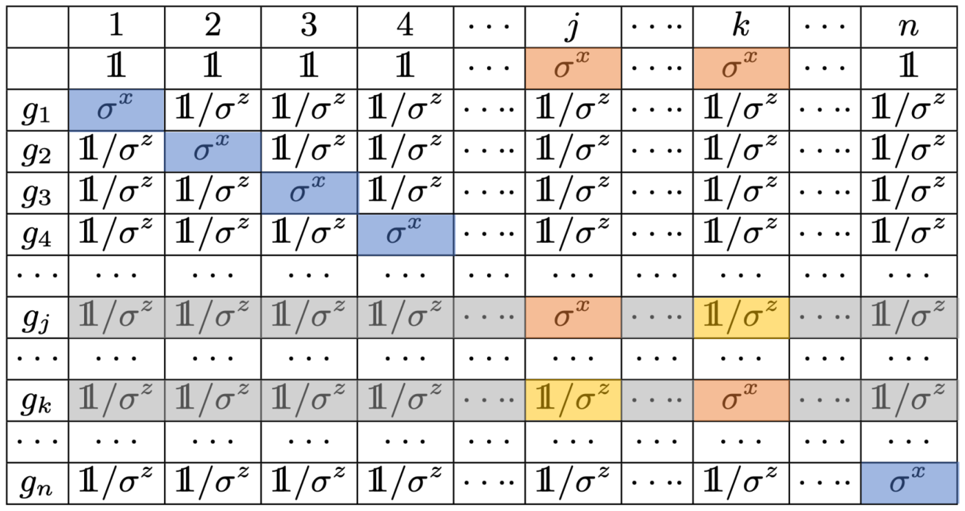
One should notice that can be rewritten into
| (38) | |||||
For the term , the th position of is . However, this position of any other is or , which means this position of is or , a traceless matrix. Furthermore, since the trace of a tensor is zero if any position in this tensor is traceless, one can find that for any .
With respect to the term , the similar analysis tells us that the only possible non-zero term is , namely,
| (39) |
In the case that , the equation above reduces to , which equals to 1 since (see Fig. 7). For , the only case that can make above equation non-zero is the multiplication of and is . However, the th, th positions of and are (orange boxes in Fig. 7), respectively. To make it happen, the th position of and th position of have to be too (yellow boxes in Fig. 7), which means and cannot be neighbors. Next, all the other positions (apart from th, th) of and have to be the same, indicating that th and th qubit must have the same neighborhood, i.e., . In the mean time, the condition also includes the requirement that , are not neighbors as the neighbor qubits cannot share the same neighborhood as they have each other in the neighborhood. Hence, the only case that make () non-zero is that . The off-diagonal entries of QFIM can then be expressed by
| (40) |
In the case that the parameter number is less than , the parameterization the operator can be written as
| (41) |
where is the set of vertices that are used to encode . The QFIM can be written as
| (42) |
where
| (43) |
Therefore, the diagonal element of the QFIM satisfies the value of the QFI in the form of a subgraph . For , we can find that the QFIM is not necessarily invertible. For Pauli Y case, the off-diagonal entries of QFIM can then be expressed by
| (44) |
And the diagonal entries of QFIM can then be expressed by for all . For Pauli- case, the QFIM can be obtained
| (45) |
where is the -dimension identity matrix.
Secondly, the parameterization process for is performed via the operator
| (46) |
where , and the Hermitian operators are the generator of the , and for all with the parameters . The element of QFIM can be expressed by
| (47) |
We can find that the QFIM is parameter independent, the quantum Cramér-Rao bound satisfies
| (48) |
where is the constant number.
Appendix B Proof the Pauli operators on SU(2)
Next, we proof the for . To proof , we only need to proof , , and , where is the collective operators. The density matrix has the expression ( 38). So we can only proof the .
Firstly, for the term , the th position of is . However, this position of any other is or , which means this position of is or , a traceless matrix. Furthermore, since the trace of a tensor is zero if any position in this tensor is traceless, one can find that for any .
Secondly, for the term , the th position of is . However, this position of any other is or , which means this position of is or , a traceless matrix. Furthermore, since the trace of a tensor is zero if any position in this tensor is traceless, one can find that for any .
Finally, for the , the th position of the is . However, this position of any other is or , whcih means this position of is or , the are the traceless matrices. Furthermore, since the trace of a tensor is zero if any position in this tensor is traceless, one can find that for any . One can find that , in which the Hermitian operator satisfies .
However, when the operators , then the is not always 0. Examples, when operators is the generators of the . The global Hamiltonian can be rewritten as , i.e., two-qubit graph state corresponds to , three-qubit graph state corresponds to , four-qubit graph state corresponds to . The is not always zero as shown in Fig. 8.
Appendix C Construct graphs with a diagonal QFIM with SU(2)
To construct graphs with a diagonal QFIM, we first define a set of basic cells for the stabilizers (denoted by ). All basic cells in satisfy (i) the QFIM is diagonal and (ii) in , any basic cell cannot be constructed by other basic cells via the single-joint connecting rule (SJCR, denoted by "-" in the following), with which the connection of any two basic cells in a graph can only share one joint vertex. Next, we define a topological number of a graph state as the number of cases in which any four vertices in this graph are the neighborhood of each other, as shown in Fig. 9(a). For example, for the graph given in Fig. 9(b), vertices 1, 2, 3, 5 (within the dashed black line) are the neighborhood, and so does vertices 1, 3, 4, 5 (within the dashed yellow line), therefore, the topological number for this graph. In the case of , we provide the following theorem.
Theorem 1. Let with and the basic cells defined in Fig. 9(c), the QFIM is the identity matrix by using constructed graphs via the SJRC.
Here we use the mathematical induction to prove the Theorem. Denote as the number of basic cells and . In the case of , the graphs are just and , and the QFIM is obviously diagonal. Recall that the single-joint connecting rule is denoted by "-", the graphs for are -, - and -. The corresponding QFIMs are also diagonal according to Eq. (40). Now we assume that, in the case of , the QFIMs of all graphs constructed by and via the single-joint connecting rule is diagonal, and in the following, we will prove the same result can be obtained for .
In the case of , all the graphs can be constructed by connecting graphs with (denoted by ) and a or . According to the single-joint connecting rule, the vertices in that can perform the connections are the free vertices (purple ones in Fig. 10(a)) in at the end and in the middle or at the end. When linking or to the free vertices in , there exist three possible scenarios, as given in Fig. 10(b) for and Fig. 10(c) for . In all these six scenarios, the joint vertices (labeled as 2) between and () have new nearest neighbors due to the connection, however, their next nearest neighbors do not change. Therefore, they will not contribute non-zero off-diagonal entries of the QFIM since the QFIM for is diagonal. With respect to the new vertices (labeled as 3) in the graph, the nearest neighbors of the joints (labeled as 1) in are now the next nearest neighbors of vertices 3, however, they do not share the same neighborhood since vertices 1 always connects to other vertices (including other vertices 1) in besides vertices 2, yet vertices 3 only connect to vertices 2 or other vertices 3. Hence, the connection between and () via the single-joint connecting rule does not create pairs of vertices that share the same neighborhood, and the QFIM of the new graph then still keeps diagonal. The theorem is proved.
Appendix D Calculation of the QFIM with simultaneous estimation
We consider the canonical case of phase estimation, where an unknown phase is encoded using non-interacting Hamiltonian, and the unknown parameter is , the unitary operator can be written as
| (49) |
where , and is the generator of the . The operators are shown in Appendix F. For any pure quantum state, the QFIM can reads
| (50) |
where , and is the covariance matrix between the generator and with parameters . is the density matrix of the graph state as shown in the Eq. (34). And being aware of the equation
| (51) |
where is the Hermitian operator, and the Hermitian generator can then be expresses by
where is the superoperator. For three-qubit graph state of the unitary parameterization on , the generators can be written as
| (52) | ||||
where and . For this case, the QFIM depends on the parameter values, In the limit , the entries of QFIM can then be expressed by
| (53) |
An example is given below to show our results. Here we rewrite the Hamiltonian as with , and the operators are the collective operators. The QFIM is
| (54) |
Here, the and . According to the Taylor expansion of trigonometric functions, the element of the QFIM with three-qubit complete graph state can be written as
In the limit , for all , the QFIM is
| (55) |
We can find that that the precision limit of the three parameter estimaiton is with the global estimation on the dynamic.
However, when the generators satisfies , and we set the Hamiltonian is for all . In this case, we can find the QFIM are
where the subscript of the QFIM indicates that the Hamiltonian operator is , respectively. One can find that the precision limit of the three-parameter estimaiton is with the local estimation on the .
Appendix E Unitary multiparameter estimation: saturating the quantum Cramér-Rao Bound
Now we prove the quantum Cramér-Rao bound could be saturated in the scenes we are considering. For the unitary processing with a pure probe graph state , the necessar and sufficient condition for the attainability of quantum multiparameter Cramér-Rao bound is Liu2020
| (57) |
where is the symmetric logarithmic derivative (SLD) with respect to parameter , in which is defined by . Next, we now proof the above bound equal to
| (58) |
with the initial graph state . Here, the Hermitian operator is with parameter . And being aware of the Eq. (51), the Hermitian operator can then be expressed by
| (59) |
and one can find
| (60) |
One can find , we find
| (61) |
where
| (62) |
The SLD formula is obtained from the fact for a pure state, then . Compared this equation to the definition equation, it can be seen that .
| (63) |
where
which implies a sufficient but not necessary condition
| (64) |
We can find
| (65) |
We prove the equivalence of the two conditions based on SLD and the Hermitian operator . Next, We proof that
| (66) |
base on the equation , that is to prove
| (67) |
The quantum graph state is the pure state after unitary evolution , which can be written as . We can reconstruct QFIM by the and with parameter for all . In general, the states are not orthogonal to the quantum state . We can construct the matrix
| (68) | |||||
| (69) |
where . It is noticed that, according to Eq. (53), the QFIM is the real and symmetry matrix. The operator is the Hermitian operator, that is the real number, we can find is always the real number.
Appendix F The generators of the SU(N)
References
- (1) D. B. West, Introduction to Graph Theory, (Prentice Hall, Upper Saddle River, NJ, 2001).
- (2) R. Diestel, Graph Theory (Prentice Hall, Upper Saddle River, NJ, 2001).
- (3) R. Raussendorf, D. E. Browne, and H. J. Briegel, Measurement-based quantum computation on cluster states, Phys. Rev. A 68, 022312 (2003).
- (4) W. Dür, H. Aschauer, and H. J. Briegel, Multiparticle Entanglement Purification for Graph States, Phys. Rev. Lett. 91, 107903(2003).
- (5) M. Grassl, A. Klappenecker, and M. Rötteler, Graphs, Quadratic Forms, and Quantum Codes, in Proceedings of the 2002 IEEE International Symposium on Information Theory, Lausanne, Switzerland, 2002, p. 45.
- (6) H.-J. Briegel and R. Raussendorf, Persistent Entanglement in Arrays of Interacting Particles, Phys. Rev. Lett. 86, 910 (2001).
- (7) M. Hein, J. Eisert and H.-J. Briegel Persistent Entanglement in Arrays of Interacting Particles, Phys. Rev. A 69, 062311 (2004).
- (8) H. Aschauer, W. Dür, and H.-J. Briegel, Multiparticle entanglement purification for two-colorable graph states, Phys. Rev. A 71, 012319 (2005).
- (9) M. Van den Nest, J. Dehaene and B. De Moor, Graphical description of the action of local Clifford transformations on graph states, Phys. Rev. A 69, 022316 (2004).
- (10) D. Gottesman, Stabilizer Codes and Quantum Error Correction, PhD thesis, CalTech,Pasadena (1997).
- (11) D. Schlingemann and R. F. Werner, Quantum error-correcting codes associated with graphs, Phys. Rev. A 65, 012308 (2001)
- (12) R. Raussendorf and H. -J. Briegel, A One-Way Quantum Computer, Phys. Rev. Lett. 86, 5188 (2001)
- (13) N. Shettell and D. Markham, Graph States as a Resource for Quantum Metrology, Phys. Rev. Lett. 124, 110502 (2020)
- (14) J. Liu, H. Yuan, X.-M. Lu, and X. Wang, Quantum Fisher information matrix and multiparameter estimation, J. Phys. A: Math. Theor. 53, 023001 (2020).
- (15) M. Szczykulska, T. Baumgratz and A. Datta, Multi-parameter quantum metrology, Adv. Phys. X 1, 621 (2016).
- (16) M. Zhang, H-M. Yu, H. Yuan, X. G. Wang, R. Demkowicz-Dobrzański, and J. Liu, QuanEstimation: An open-source toolkit for quantum parameter estimation, Phys. Rev. Research 4, 043057 (2022).
- (17) F. Albarelli, M. Barbieri, M. G. Genonie, and I. Giananifc, A perspective on multiparameter quantum metrology: From theoretical tools to applications in quantum imaging, Phys. Lett. A 384, 126311 (2020).
- (18) G. Tóth and I. Apellaniz, Quantum metrology from aquantum information science perspective, J. Phys. A: Math. Theor. 47, 424006 (2014).
- (19) V. Giovannetti, S. Lloyd, and L. Maccone, Quantum Metrology, Phys. Rev. Lett. 96, 010401 (2006).
- (20) V. Giovannetti, S. Lloyd, and L. Maccone, Quantum-enhanced measurements: beating the standard quantumlimit, Science 306,1330 (2004).
- (21) V. Giovannetti, S. Lloyd, and L. Maccone, Advances in quantum metrology, Nat. Photonics 5,222 (2011).
- (22) R. Demkowicz-Dobrzanski, M. Jarzyna, and J. Kolodynski, Chapter Four-Quantum Limits in Optical Interferometry Prog. Opt. 60, 345 (2015).
- (23) R. Demkowicz-Dobrzański, J. Kolodyński, and M. Guţä, The elusive Heisenberg limit in quantum-enhanced metrology, Nat. Commun.3, 1063 (2012).
- (24) T. Baumgratz and A. Datta, Quantum Enhanced Estimation of a Multidimensional Field, Phys. Rev. Lett.116, 030801 (2016)
- (25) L. T. Hall, G. C. G. Beart, E. A. Thomas, D. A. Simpson, L. P. McGuinness, J. H. Cole, J. H. Manton, R. E. Scholten, F. Jelezko, J. Wrachtrupet al., High spatial and temporal resolution wide-field imaging of neuron activity using quantum NV-diamond, Sci. Rep.2, 401 (2012).
- (26) M. A. Seo, A. J. L. Adam, J. H. Kang, J. W. Lee, S. C. Jeoung, Q. H. Park, P. C. M. Planken, and D. S. Kim, Fourier-transform terahertz near-field imaging of one-dimensional slitarrays: Mapping of electric-field-, magnetic-field-, and Poynting vectors, Opt. Express 15, 11781 (2007).
- (27) S. Steinert, F. Dolde, P. Neumann, A. Aird, B. Naydenov, G.Balasubramanian, F. Jelezko, and J. Wrachtrup, Highsensitivity magnetic imaging using an array of spins indiamond, Rev. Sci. Instrum.81, 043705 (2010).
- (28) L. M. Pham, D. Le Sage, P. L. Stanwix, T. K. Yeung, D.Glenn, A. Trifonov, P. Cappellaro, P. R. Hemmer, M. D. Lukin, H. Parket et al., Magnetic field imaging with nitrogen-vacancy ensembles, New J. Phys. 13, 045021 (2011).
- (29) J. Liu, X.-M. Lu, Z. Sun, and X. Wang, Quantum multi-parameter metrology with generalized entangled coherent state, J. Phys. A: Math. Theor. 49, 115302 (2016).
- (30) P. C. Humphreys, M. Barbieri, A. Datta, and I. A. Walmsley, Quantum Enhanced Multiple Phase Estimation, Phys. Rev. Lett. 111, 070403 (2013).
- (31) M. A. Ciampini, N. Spagnolo, C. Vitelli, L. Pezzé, A. Smerzi, and F. Sciarrino, Quantum-enhanced multiparameter estimation in multiarm interferometers, Sci.Rep. 6, 28881 (2016).
- (32) J.-D. Yuecoherent state, and H. Fan, Quantum-enhanced metrology for multiple phase estimation with noise, Sci. Rep. 4, 5933 (2014).
- (33) P. A. Knott, T. J. Proctor, A. J. Hayes, J. F. Ralph, P. Kok, andJ. A. Dunningham, Local versus global strategies in multi-parameter estimation, Phys. Rev. A 94, 062312 (2016).
- (34) C. N. Gagatsos, D. Branford, and A. Datta, Gaussian systems for quantum-enhanced multiple phase estimation, Phys. Rev. A 94, 042342 (2016).
- (35) L. Zhang and K. W. C. Chan, Quantum multiparameter estimation with generalized balanced multimode noon-likestates, Phys. Rev. A 95, 032321 (2017).
- (36) P. Komar, E. M. Kessler, M. Bishof, L. Jiang, A. S. Sørensen, J. Ye, and M. D. Lukin, A quantum network of clocks, Nat. Phys. 10, 582 (2014).
- (37) T. J. Proctor, P. A. Knott, and J. A. Dunningham, Multiparameter Estimation in Networked Quantum Sensors, Phys. Rev. Lett. 120, 080501 (2018).
- (38) M. Gessner, L. Pezze, and A. Smerzi, Sensitivity Bounds for Multiparameter Quantum Metrology, Phys. Rev. Lett.121, 130503 (2018)
- (39) H. D. Yuan, Sequential Feedback Scheme Outperforms the Parallel Scheme for Hamiltonian Parameter Estimation, Phys. Rev. Lett.117, 160801 (2016)
- (40) H. Imai and A. Fujiwara, Geometry of optimal estimation scheme for SU(D) channels, J. Phys. A 40, 4391 (2007)
- (41) A. Z. Goldberg, L. L. Sánchez-Soto, and H. Ferretti, Intrinsic Sensitivity Limits for Multiparameter Quantum Metrology, Phys.Rev.Lett. 127, 110501 (2021)
- (42) L. Pezzé, M. A. Ciampini, N. Spagnolo,P. C. Humphreys, A. Datta, I. A. Walmsley,M. Barbieri, F. Sciarrino, and A. Smerzi, Optimal Measurements for Simultaneous Quantum Estimation of Multiple Phases, Phys. Rev. Lett. 119, 130504 (2017).
- (43) H. Z. Chen, Y, Chen. and H. D. Yuan,, Information Geometry under Hierarchical Quantum Measurement, Phys. Rev. Lett. 128, 250502 (2022).
- (44) F. Albarelli, M. Barbieri, M. G. Genoni, and I. Gianani, A perspective on multiparameter quantum metrology: From theoretical tools to applications in quantum imaging, Phys. Lett. A 384, 126311 (2020).
- (45) J. Rubio, P. A. Knott, T. J. Proctor, and J. A. Dunningham, Quantum sensing networks for the estimation of linear functions, J. Phys. A: Math. Theor. 53, 344001 (2020).
- (46) J. A. Gross and C. M. Caves, One from many: Estimating afunction of many parameters, J. Phys. A: Math. Theor. 54, 014001 (2021).
- (47) D. Triggiani, P. Facchi, and V. Tamma, Heisenberg scaling precision in the estimation of functions of parameters in linear optical networks, Phys.Rev. A 104, 062603 (2021).
- (48) C. W. Helstrom, Quantum Detection and Estimation Theory (New York: Academic, 1976).
- (49) A. S. Holevo, Probabilistic and Statistical Aspects of Quantum Theory (Amsterdam: North-Holland, 1982).
- (50) K. Matsumoto, A new approach to the Cramér-Rao-type bound of the pure-state model, J. Phys. A: Math. Gen. 35, 3111 (2002).
- (51) H. Zhu, Information complementarity: A new paradigm fordecoding quantum incompatibility, Sci. Rep.5, 14317 (2015).
- (52) T. Heinosaari, T. Miyadera, and M. Ziman, An invitation to quantum incompatibility, J. Phys. A: Math. Theor. 49, 123001 (2016).
- (53) S. Ragy, M. Jarzyna, and R. Demkowicz-Dobrzański, Compatibility in multiparameter quantum metrology, Phys.Rev. A 94, 052108 (2016).
- (54) J. A. Omolo, Determining SU(N) symmetry group generators, ResearchGate-Preprint, (2018).
- (55) H. Haber, Useful relations among the generators in the defining and adjoint representations of SU(N), SciPost Phys. Lect. Notes, 21, (2021).
- (56) A. S. Sørensen and K. Mølmer, Entanglement and Extreme Spin Squeezing, Phys. Rev. Lett. 86, 4431 (2001)
- (57) O. Gühne, G. Tóth, and H. J. Briegel, Multipartite entanglement in spin chains, New J. Phys. 7, 229 (2005)
- (58) W. K. Wootters, Entanglement of Formation of an Arbitrary State of Two Qubits, Phys. Rev. Lett. 80, 2245 (1998)
- (59) P. Hyllus, W. Laskowski, R. Krischek, C. Schwemmer,W. Wieczorek, H. Weinfurter, L. Pezzé, and A. Smerzi, Fisher information and multiparticle entanglement, Phys. Rev. A 85, 022321 (2012)
- (60) G. Tóth, Multipartite entanglement and high-precision metrology, Phys. Rev. A 85, 022322 (2012)
- (61) T. E. Lee, F. Reiter, and N. Moiseyev, Entanglement and Spin Squeezing in Non-Hermitian Phase Transitions, Phys. Rev. Lett. 113, 250401 (2014)