The Semi-implicit DLN Algorithm for the Navier Stokes Equations
Abstract
Dahlquist, Liniger, and Nevanlinna design a family of one-leg, two-step methods (the DLN method) that is second order, and stable for arbitrary, non-uniform time steps. Recently, the implementation of the DLN method can be simplified by the refactorization process (adding time filters on backward Euler scheme). Due to these fine properties, the DLN method has strong potential for the numerical simulation of time-dependent fluid models. In the report, we propose a semi-implicit DLN algorithm for the Navier Stokes equations (avoiding non-linear solver at each time step) and prove the unconditional, long-term stability and second-order convergence with the moderate time step restriction. Moreover, the adaptive DLN algorithms by the required error or numerical dissipation criterion are presented to balance the accuracy and computational cost. Numerical tests will be given to support the main conclusions.
keywords
Refactorization, -stability, second-order, time adaptivity, semi-implicitAMS
65M12, 35Q30, 76D051 Introduction
In the simulation of time-dependent fluid models, various time-stepping schemes have been constructed based on stability and consistency. The backward Euler method, unconditionally stable and easily implemented, can only have first-order accuracy [22, 37, 51, 52]. The trapezoidal rule or two-step backward difference method (BDF2) are both second-order accurate and widely used in computational fluid dynamics [26, 27, 28, 29, 43, 3, 11, 18, 19, 47, 54]. However, the trapezoid rule with some unfavorable combinations of time steps leads to instability of the numerical solutions [16, 53]. The variable-step BDF2 method only has conditional stability if the time step ratio is small enough [8, 9, 20, 21, 30, 31].
Dahlquist, Liniger, and Nevanlinna propose a one-parameter family of one-leg, two-step method (thus the DLN method herein) which is -stable (non-linear stable) [13, 14, 15, 16] and second-order accurate under arbitrary time grids. To our knowledge, the DLN method is the only time-stepping algorithm possessing these two properties under arbitrary time step sequence. Hence its essential properties of stability and consistency have been carefully studied and explored in [45, 46]. Recently the variable step DLN method has been applied to the unsteady Stoke/Darcy model and Navier Stokes equations (NSE) and performs well in specific test problems [44, 50, 49].
Given the initial value problem:
| (1.1) |
for , and . The family of one-leg, two-step DLN method (with parameter ), applying to (1.1) is written
| (DLN) |
Here are the time grids on interval and is the DLN solution to . The coefficients in (DLN) are
The step variability is the function of two step size. is the average time step. Given sequence , we denote
for convenience in the remaining paragraphs. Then the DLN method in (DLN) can be shorten
Herein we propose the variable-step, semi-implicit DLN algorithm for NSE and present a detailed numerical analysis of stability and convergence. Let the open, connected and bounded set () be the domain, the fluid velocity , pressure and the source in the NSE are governed by the following system
| (1.2) | |||
Let and are the numerical solutions to velocity and pressure respectively on certain finite element space with diameter , the fully-implicit DLN algorithm for NSE approximate the non-linear term at by [44], which results in two main disadvantages of the algorithm:
- i.
the rigorous time step restriction like for convergence,
- ii.
the non-linear solver in each time step computation.
The above time step restriction in error analysis arises from the use of the discrete Grnwall inequality [35, p.369] and would be very strict even under moderate viscosity value (like )11 1 To our knowledge, the restriction can not be avoided as long as the fully-implicit, time-stepping methods are applied.. Fixed point iteration and Newton’s iteration are two common choices for non-linear solvers. Fixed point iteration is easily implemented while Newton’s iteration possesses fast convergence. However, they usually cost more than solving a linear system and have the risk of divergence if the initial value for the iteration is poorly guessed.
To address the two issues, we extend Baker’s idea [1] and propose the semi-implicit DLN scheme for NSE. The essence of the idea is to extrapolate the first in the non-linear term by its second-order extrapolation in time (the linear combination of and ). In return, the non-linear solver at each time step is replaced by a linear system. Meanwhile, the strict time step restriction for convergence can be released. In addition, we simplify the DLN implementation by the refactorization process (pre- and post-process on backward Euler scheme) and improve the computational efficiency by the corresponding time adaptivity algorithms.
The paper is organized as follows. Necessary notations and preliminaries are given in Section 2. In section 3, we propose the semi-implicit DLN algorithm for NSE and its equivalent implementation by the refactorizaion process. In section 4.1, we will show that the numerical solution is long-term, unconditionally stable. The variable step error analysis with the loose time step restriction is given in Section 4.2. The time adaptive algorithms (using error or numerical dissipation criterion) in Section 5 are provided to reduce the computational cost. In Section 6, the Taylor-Green benchmark problem [55] is to confirm the second-order convergence. The unconditional stability of the variable step DLN and the advantage of time adaptivity are verified in the revised Taylor-Green problem and the 2D offset problem [37].
1.1 Related Work
Semi-implicit schemes are effective ways to simulate non-linear, time-dependent fluid models. Baker studied the semi-implicit Crank-Nicolson method and applied it to NSE [1] early. Baker, Dougalis, and Karakashian increase the accuracy of numerical solutions by use of the three-step backward difference method coupled with extrapolation for non-linear terms [2]. Girault and Raviart prove the convergence of general linear two-step semi-implicit algorithms for NSE [24]. They solve the two-dimensional NSE by a fully discrete two-level finite element method: Crank-Nicolson extrapolation scheme on spatial-time coarse grids and backward Euler scheme on fine grids [34]. Labovsky, Layton, Manica, Neda, and Rebholz add artificial viscosity stabilization to extrapolated trapezoidal finite-element method for NSE, leading to a more easily solvable linear system at each time step [42]. Ingram offers a detailed numerical analysis of the semi-implicit Crank-Nicolson scheme for NSE and proves the convergence of both velocity and pressure [36].
Time adaptivity based on certain criteria (required local truncation error, minimum numerical dissipation, etc.) is an optimal choice to treat the conflicts between time accuracy and efficiency. Inspired by the pioneering work of Gear [23], Kay, Gresho, Griffiths, and Silvester implement the trapezoidal scheme for NSE in a memory efficient way and estimate the error in time by the explicit two-step Adams Bashforth method (AB2 method) in the time adaptivity [27, 29, 26, 40]. John and Rang propose diagonal-implicit RK methods (DIRK methods) with an embedding lower-order scheme for adaptivity and implement this algorithm for 2D laminar flow around a cylinder [39]. Guzel and Layton add the time filter to the backward Euler method to increase the accuracy of numerical solutions [32]. The corresponding BE-filter adaptivity is applied to various fluid models [12, 17, 48]. Recently Bukač, Burkardt, Seboldt, and Trenchea refactorize the midpoint rule and adjust time steps by the revised AB2 method in fluid-structure interaction problems [7, 4, 5, 6]. The numerical dissipation criterion for adaptivity, proposed by Capuano, Sanderse, De Angelis, and Coppola in [10], has been tested in the DLN simulations of the NSE and the coupled Stokes-Darcy model [44, 49].
2 Preliminaries
Let () be the domain. For , is the normed linear space containing Lebesgue measurable function such that is integragle. For , the Sobolev space with usual norm contains all Lebesgue measurable functions whose weak derivatives up to -th belong to and is the usually space. and denote the -norm and -inner product. The space with norm and semi-norm denotes the Sobolev space with . The velocity space and the pressue space for the NSE in (1.2) are
The divergence-free space for the velocity is
For any function , the norm and semi-norm are define
is the dual space of with the dual norm
| (2.1) |
We need the Bochner space on the time interval
and the discrete Bochner space with the time grids on the time interval
where the corresponding discrete norms are
| (2.2) |
The discrete norm in (2.2) is the form of Riemann sum in which the function is evaluated at . For any , we define the skew-symmetric, non-linear operator
| (2.3) |
We apply divergence theorem and integration to (2.3)
Thus if , . We have the following lemma about the bounds of the operator .
Lemma 1.
For any ,
| (2.4) | |||
| (2.5) |
Moreover, if ,
| (2.6) |
Proof.
See [36, p.273-275]. ∎
For spatial discretization, and are certain finite element spaces for velocity and pressure respectively based on the edge-to-edge triangulation of domain (with the maximum diameter of the triangles ). and satisfy the discrete inf-sup condition, i.e.
| (2.7) |
for some positive constant . Typical examples of such finite element spaces are Taylor-Hood element spaces and Mini element spaces. The approximation theorem for and is
| (2.8) |
where and are the polynomial degrees of and respectively. The inverse inequality for is
| (2.9) |
The discrete divergence-free space is
For any pair , the Stokes projection is defined as the solution to the problem
The Stokes projection has the following approximations (see [25, 38] for proof)
| (2.10) |
3 The algorithm
Let and be the numerical solutions of velocity and pressure respectively. Then the semi-implicit DLN algorithm for the NSE in (1.2) is: given two previous solutions , , find and such that for all
| (3.1) |
where the second-order, linear extrapolation for is
The above semi-implicit DLN algorithm in (3.1) can be simplified by the following refactorizaion process (See [45] for the proof of equivalence)
Step 1. Pre-possess:
Step 2. Semi-implicit backward Euler solver: solve for and
Step 3. Post-possess:
where the coefficents in the refactorizaion process are
4 Numerical Analysis
For numerical analysis, we need the following two lemma about the stability and consistency of the DLN method.
Lemma 2.
Let be the inner product space over with the inner product and the induced norm . For any sequence in , and
| (4.1) |
where the -norm is
| (4.2) |
and the coefficents are
| (4.3) |
By the above identity in (4.1), the whole family of variable step, one-leg (DLN) methods are G-stable (see [13, p.2] for the definition).
Lemma 3.
Given Banach space with the norm , time grids on time interval and the mapping , denotes and represents second-order, linear extrapolation of in time, i.e.
| (4.4) |
If the mapping is smooth enough about variable , then for any
| (4.5) |
Moreover, if there exists constants such that the ratio of time steps satisfies
then
| (4.6) |
Proof.
Using Taylor theorem and expanding , and at time . ∎
4.1 Stability Analysis
Theorem 4.
Proof.
Remark 1.
We define the numerical dissipation and viscosity dissipation of the semi-implicit DLN algorithm in (3.1) at time
4.2 Error Analysis
Let and be the polynomial degree of and respectively and
Let and be the exact velocity and pressure of the NSE in (1.2) at time . We need the following upper and lower bound for the ratio of time steps: there are positive constants and such that
| (4.9) |
Theorem 5.
Proof.
The exact solutions of NSE at time satisfy:
| (4.11) | |||
where is second-order, linear extrapolation of in (4.4) and the truncation error is
Let be velocity component of the Stokes projection of onto . We set
and decompose the error of velocity to be
| (4.12) |
We restrict in (3.1) and subtract (4.11) from the first equation of (3.1)
| (4.13) | ||||
We set in (4.13) and use the -stability identity in (4.1),
| (4.14) |
By Cauchy-Schwarz inequality, Poincar inequality, Young’s equality, (2) and (2.10) ( vanishes since in the Stokes projection)
| (4.15) | ||||
By Holder’s inequality
| (4.16) | ||||
| (4.17) |
By the definition of the Stokes projection, . We set
The non-linear terms in (4.14) become
By (2.4), (2.5), (2.9) and (2.10), Poincar inequality and step requirement in (4.9)
| (4.18) | ||||
We apply Young’s inequality to all non-linear terms in (4.18)
| (4.19) | ||||
By (2), triangle inequality and (4.5) in Lemma 3
(4.19) becomes
| (4.20) | ||||
We set to be projection of onto in (4.14) and use (2)
| (4.21) |
Now we treat : by (4.5) and (4.6) in Lemma 3
| (4.22) | ||||
| (4.23) | ||||
| (4.24) | ||||
| (4.25) | ||||
We combine (4.17), (4.20), (4.21), (4.22), (4.23), (4.24), (4.25) and sum (4.14) over from to
| (4.26) | ||||
By the definition of the -norm in (4.2), (4.26) becomes
| (4.27) | ||||
By the discrete Grnwall inequality without restrictions ([35, p.369]), (4.27) becomes
| (4.28) |
where
| (4.29) |
By triangle inequality and (4.5) in Lemma 3, (4.28) can be simplifed
By triangle inequality, (2), (4.5) in Lemma 3 and (4.28)
| (4.30) | ||||
| (4.31) | ||||
| (4.32) | ||||
which implies (4.10). ∎
Theorem 6.
Proof.
Let be Stokes projection of onto . We set
We let in (4.13). By the -stability identity in (4.1), (4.13) becomes
| (4.36) |
By Cauchy Schwarz inequality, Young’s inequality, (2), (2.10) and Hlder’s inequality
| (4.37) | ||||
By the definition of Stokes projection and the fact that
For :
| (4.38) | ||||
| (4.39) | ||||
| (4.40) | ||||
| (4.41) | ||||
For non-linear terms
By (2.4), (2.6) and inverse inequality in (2.9)
Thus
| (4.42) | ||||
By Cauchy-Schwarz inequality, Young’s inequality, Poincar inequality, (2), (2.10) and (4.5)
| (4.43) | ||||
| (4.44) | ||||
| (4.45) | ||||
| (4.46) | ||||
By (4.43), (4.44), (4.45) and (4.46), (4.42) becomes
| (4.47) | ||||
We use integration by parts and (4.5) in Lemma 3
| (4.48) | ||||
We combine (4.37), (4.38), (4.39), (4.40), (4.41), (4.47), (4.48) and sum (4.36) over from to
| (4.49) | ||||
Since
we use (4.32) in the proof of Theorem 5 to obtain
| (4.50) |
where
and is in (4.2). We apply (4.50) and discrete Gronwall inequality to (4.49)
| (4.51) | ||||
where
By the time-diameter condition in (4.33), is bounded. Thus
| (4.52) | ||||
Combining Theorem 5 and (4.52), we have (4.34). By (2), (2.10) and Hlder’s inequality
| (4.53) |
By (4.51) and (4.2) and triangle inequality
| (4.54) | ||||
which implies (4.35). ∎
Theorem 7.
Suppose the velocity and pressure of the NSE in (1.2) satisfy
and the body force , then under the time step bounds in (4.9) and the time-diameter condition in (4.33), the pressure component by the algorithm in (3.1) satisfy
| (4.55) |
Moreover for constant time-stepping DLN algorithm with parameter and constant time step , we have
| (4.56) |
Proof.
Let be Stokes projection of onto . We set
We let in (4.11) and subtract (4.11) from the first equation of (3.1)
| (4.57) |
where is the projection of onto . By (2.4) and Poincar inequality
| (4.58) | ||||
By Cauchy-Schwarz inequality, (4.5) and (4.6) in Lemma 3
| (4.59) | ||||
| (4.60) | ||||
| (4.61) |
By (2.4), (4.5) in Lemma 3 and Poincar inequality
| (4.62) | ||||
We combine (4.59), (4.60), (4.61) and (4.62)
| (4.63) |
| (4.64) |
By (2.7),(4.58), (4.2) and (4.2)
| (4.65) | ||||
By triangle inequality, (2) and (4.65)
| (4.66) | ||||
By (4.5) in Lemma 3, (4.32), (4.52), (4.54) and (4.66)
| (4.67) | ||||
which implies (4.55). For constant step case, and the coefficients are
By triangle inequality and (2)
| (4.68) | ||||
By Cauchy-Schwarz inequality and (4.5) in Lemma 3
| (4.69) | ||||
The bound of term is given in (4.67). Thus we combine (4.67), (4.68) and (4.69) to obtain
| (4.70) | ||||
which implies (4.56).
∎
5 Implementation of Adaptive DLN Algorithm
We present two ways of time adaptivity for the whole family of DLN methods. The first way is to use the local truncation error (LTE) criterion: we apply the revised AB2 method (herein AB2-like method) to estimate the error of the DLN scheme for NSE and adjust the time step according to the ratio of the required tolerance and the estimator. The second way is to adapt the time step to control the numerical dissipation.
5.1 Local Truncation Error Criterion
Given four previous solutions ,
the AB2-like solution for NSE at time is
| (5.1) | ||||
and the estimators are
| (Absolute estimator) | ||||
| (Relative estimator) |
where
| (5.2) | ||||
We refer to [46] for the derivation of the AB2-like method in (5.1) and the estimator in (Absolute estimator) and (Relative estimator). We use the step controller proposed by Hairer and Wanner in [33] to adjust the next time step
| (5.3) |
where Tol is the required tolerance and the safety factor is selected to minimize the number of step rejections. If , then the DLN solution is rejected and the current step is adjusted by (5.3) for recomputing. We summarize the above adaptive DLN algorithm in Algorithm 1
5.2 Numerical Dissipation Criterion
The algorithm proposed by Capuano, Sanderse, De Angelis and Coppola [10] calibrates the step size to ensure the ratio of numerical dissipation and viscosity under the required value and its effect on the fully-implicit DLN scheme has been tested in [44]. Given the tolerance , the maximum time step , the minimum time step , we compute the DLN solution and the ratio of numerical dissipation and viscosity
If , we accept the current solutions and double the time step. Otherwise, we halve the time step for recomputing. We summarize the algorithm in Algorithm 2.
6 Numerical Tests
We apply the semi-implicit DLN algorithm in (3.1) with for all numerical tests. is suggested in [16] to balance the stability and local truncation error. is recommended in [41] for stability at infinity (a property similar to -stability). reduces to the midpoint rule. We use software FreeFem++ and Taylor-Hood () finite element space for programming.
6.1 Convergence Test
We use the Taylor-Green benchmark problem [55] to verify that the semi-implicit DLN algorithm is second-order accurate. In addition, its efficiency over the fully-implicit algorithm can be observed. The exact solutions in the domain are
| (6.1) | |||
We set the parameters , . The initial value, boundary condition and source function are determined by the exact solutions in (6.1). We require that the constant time step and mesh diameter are the same to satisfy the time-diameter condition in (4.33). We simulate the problem over the time interval . The convergence rate is calculated by
The results of the semi-implicit DLN algorithm (with constant time step) are given in Tables 1, 2, 3, 4, 5 and 6. We see that the semi-implicit DLN has third-order convergence in velocity and second-order convergence in pressure for all three values. Hence the semi-implicit DLN scheme has much better performance in the Taylor-Green problem than the theories in Subsection 4.2 suggest. Then we apply the fully-implicit DLN scheme to the same problem and use fixed point iteration to solve the non-linear system at each time step. The error and convergence rate are given in Tables 7, 8, 9, 10, 11 and 12. From the above tables, we observe that the semi-implicit DLN algorithm outperforms the fully-implicit algorithm for all three values in this test problem: The two schemes have almost the same error magnitude but the fully-implicit scheme takes twice the time to finish the simulation since the fully-implicit scheme takes two iterations on average at each time step.
| Time(s) | |||||||
|---|---|---|---|---|---|---|---|
| 3.9474e-4 | - | 4.6605e-2 | - | 2.7357e-3 | - | 8.1388 | |
| 2.8230e-5 | 3.8056 | 6.4712e-3 | 2.8484 | 7.0563e-4 | 1.9550 | 64.792 | |
| 2.1586e-6 | 3.7091 | 8.5120e-4 | 2.9265 | 1.7820e-4 | 1.9854 | 572.01 | |
| 1.9754e-7 | 3.4499 | 1.0916e-4 | 2.9630 | 4.4717e-5 | 1.9946 | 4482.08 | |
| 2.1700e-8 | 3.1864 | 1.3823e-5 | 2.9814 | 1.1180e-5 | 1.9999 | 36165.2 |
| Time(s) | |||||||
|---|---|---|---|---|---|---|---|
| 2.3215e-4 | - | 2.6161e-2 | - | 1.3270e-3 | - | 8.1388 | |
| 1.6575e-5 | 3.8080 | 3.3174e-3 | 2.9793 | 3.1602e-4 | 2.0700 | 64.792 | |
| 1.4593e-6 | 3.5057 | 4.1514e-4 | 2.9984 | 7.6861e-5 | 2.0397 | 572.01 | |
| 1.5827e-7 | 3.2048 | 5.1850e-5 | 3.0012 | 1.8945e-5 | 2.0204 | 4482.08 | |
| 1.9010e-8 | 3.0576 | 6.4763e-6 | 3.0011 | 4.7026e-6 | 2.0103 | 36165.2 |
| Time(s) | |||||||
|---|---|---|---|---|---|---|---|
| 4.0528e-4 | - | 4.7930e-2 | - | 3.0208e-3 | - | 8.3926 | |
| 2.9297e-5 | 3.7901 | 6.7547e-3 | 2.8270 | 7.8296e-4 | 1.9479 | 66.443 | |
| 2.2303e-6 | 3.7155 | 8.9557e-4 | 2.9150 | 1.9809e-4 | 1.9827 | 550.33 | |
| 2.0105e-7 | 3.4716 | 1.1533e-4 | 2.9570 | 4.9746e-5 | 1.9935 | 4670.8 | |
| 2.1835e-8 | 3.2029 | 1.4635e-5 | 2.9783 | 1.2439e-5 | 1.9997 | 36117.4 |
| Time(s) | |||||||
|---|---|---|---|---|---|---|---|
| 2.3063e-4 | - | 2.5960e-2 | - | 1.4135e-3 | - | 8.3926 | |
| 1.6544e-5 | 3.8012 | 3.3095e-3 | 2.9716 | 3.2890e-4 | 2.1036 | 66.443 | |
| 1.4587e-6 | 3.5036 | 4.1515e-4 | 2.9949 | 7.8584e-5 | 2.0653 | 550.33 | |
| 1.5816e-7 | 3.2052 | 5.1876e-5 | 3.0005 | 1.9165e-5 | 2.0357 | 4670.8 | |
| 1.8980e-8 | 3.0588 | 6.4789e-6 | 3.0012 | 4.7299e-6 | 2.0186 | 36117.4 |
| Time(s) | |||||||
|---|---|---|---|---|---|---|---|
| 4.1609e-4 | - | 4.9275e-2 | - | 3.2988e-3 | - | 8.1731 | |
| 3.0244e-5 | 3.7821 | 7.0048e-3 | 2.8144 | 8.5923e-4 | 1.9408 | 65.027 | |
| 2.2919e-6 | 3.7220 | 9.3311e-4 | 2.9082 | 2.1772e-4 | 1.9806 | 527.63 | |
| 2.0408e-7 | 3.4893 | 1.2046e-4 | 2.9535 | 5.4716e-5 | 1.9924 | 4598.7 | |
| 2.1951e-8 | 3.2168 | 1.5306e-5 | 2.9764 | 1.3687e-5 | 1.9991 | 36536.1 |
| Time(s) | |||||||
|---|---|---|---|---|---|---|---|
| 2.3657e-4 | - | 2.6577e-2 | - | 3.0674e-3 | - | 8.1731 | |
| 1.6833e-5 | 3.8129 | 3.3987e-3 | 2.9672 | 8.1328e-4 | 1.9152 | 65.027 | |
| 1.4761e-6 | 3.5115 | 4.3047e-4 | 2.9810 | 2.0835e-4 | 1.9648 | 527.63 | |
| 1.5887e-7 | 3.2159 | 5.4163e-5 | 2.9905 | 5.2629e-5 | 1.9851 | 4598.7 | |
| 1.8995e-8 | 3.0642 | 6.7926e-6 | 2.9953 | 1.3195e-5 | 1.9959 | 36536.1 |
| Time(s) | |||||||
|---|---|---|---|---|---|---|---|
| 3.9446e-4 | - | 4.6505e-2 | - | 2.7694e-3 | - | 15.605 | |
| 2.8227e-5 | 3.8047 | 6.4700e-3 | 2.8455 | 7.1375e-4 | 1.9561 | 125.958 | |
| 2.1586e-6 | 3.7089 | 8.5118e-4 | 2.9262 | 1.8025e-4 | 1.9854 | 1032.9 | |
| 1.9754e-7 | 3.4499 | 1.0916e-4 | 2.9630 | 4.5231e-5 | 1.9946 | 8796.17 | |
| 2.1700e-8 | 3.1864 | 1.3823e-5 | 2.9814 | 1.1309e-5 | 1.9999 | 71983.6 |
| Time(s) | |||||||
|---|---|---|---|---|---|---|---|
| 2.3156e-4 | - | 2.6098e-2 | - | 1.3308e-3 | - | 15.605 | |
| 1.6574e-5 | 3.8044 | 3.3170e-3 | 2.9760 | 3.1649e-4 | 2.0721 | 125.958 | |
| 1.4593e-6 | 3.5055 | 4.1514e-4 | 2.9982 | 7.6911e-5 | 2.0409 | 1032.9 | |
| 1.5827e-7 | 3.2048 | 5.1850e-5 | 3.0011 | 1.8948e-5 | 2.0211 | 8796.17 | |
| 1.9009e-8 | 3.0576 | 6.4763e-6 | 3.0011 | 4.7022e-6 | 2.0107 | 71983.6 |
| Time(s) | |||||||
|---|---|---|---|---|---|---|---|
| 4.0498e-4 | - | 4.7831e-2 | - | 3.0555e-3 | - | 18.7007 | |
| 2.9293e-5 | 3.7892 | 6.7535e-3 | 2.8243 | 7.9133e-4 | 1.9490 | 149.992 | |
| 2.2302e-6 | 3.7153 | 8.9555e-4 | 2.9148 | 2.0021e-4 | 1.9828 | 1192.33 | |
| 2.0105e-7 | 3.4715 | 1.1533e-4 | 2.9570 | 5.0276e-5 | 1.9936 | 9766.42 | |
| 2.1835e-8 | 3.2029 | 1.4635e-5 | 2.9783 | 1.2572e-5 | 1.9997 | 71773.7 |
| Time(s) | |||||||
|---|---|---|---|---|---|---|---|
| 2.2951e-4 | - | 2.5844e-2 | - | 1.4177e-3 | - | 18.7007 | |
| 1.6541e-5 | 3.7944 | 3.3086e-3 | 2.9655 | 3.2947e-4 | 2.1053 | 149.992 | |
| 1.4587e-6 | 3.5033 | 4.1514e-4 | 2.9945 | 7.8653e-5 | 2.0666 | 1192.33 | |
| 1.5816e-7 | 3.2052 | 5.1876e-5 | 3.0005 | 1.9172e-5 | 2.0365 | 9766.42 | |
| 1.8980e-8 | 3.0588 | 6.4789e-6 | 3.0012 | 4.7302e-6 | 2.0190 | 71773.7 |
| Time(s) | |||||||
|---|---|---|---|---|---|---|---|
| 4.1578e-4 | - | 4.9177e-2 | - | 3.3032e-3 | - | 18.9342 | |
| 3.0240e-5 | 3.7813 | 7.0035e-3 | 2.8118 | 8.5935e-4 | 1.9425 | 157.133 | |
| 2.2919e-6 | 3.7219 | 9.3310e-4 | 2.9080 | 2.1773e-4 | 1.9807 | 1214.16 | |
| 2.0408e-7 | 3.4893 | 1.2046e-4 | 2.9534 | 5.4718e-5 | 1.9925 | 8492.7 | |
| 2.1951e-8 | 3.2168 | 1.5306e-5 | 2.9764 | 1.3687e-5 | 1.9992 | 71309.7 |
| Time(s) | |||||||
|---|---|---|---|---|---|---|---|
| 2.3141e-4 | - | 2.6100e-2 | - | 3.0611e-3 | - | 18.9342 | |
| 1.6803e-5 | 3.7837 | 3.3893e-3 | 2.9450 | 8.1693e-4 | 1.9058 | 157.133 | |
| 1.4757e-6 | 3.5092 | 4.3010e-4 | 2.9782 | 2.0943e-4 | 1.9637 | 1214.16 | |
| 1.5887e-7 | 3.2155 | 5.4145e-5 | 2.9898 | 5.2906e-5 | 1.9850 | 8492.7 | |
| 1.8995e-8 | 3.0641 | 6.7917e-6 | 2.9949 | 1.3264e-5 | 1.9959 | 71309.7 |
6.2 Adaptive DLN Algorithms for Revised Taylor-Green Problem
We apply adaptive semi-implicit DLN algorithms in Section 5 to the revised Taylor-Green problem in the domain . The exact solutions are
| (6.2) | |||
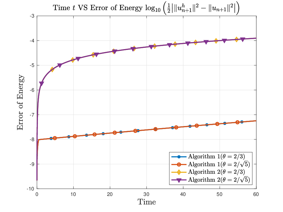
We set and . The exact solutions in (6.2) make the problem more difficult since the Reynolds number is much larger and the energy has an increasing pattern. We use both Algorithm 1 and Algorithm 2 to solve the problem over the time interval . For Algorithm 1, we use the relative estimator in (Relative estimator) and set tolerance and the safety factor . For Algorithm 2, we set for . The value of is chosen to balance accuracy and efficiency. For both algorithms, we set the minimum time step , the maximum time step , the initial time step and the mesh diameter . The initial value, boundary value and body force are decided by the exact solutions. We measure the performance of two algorithms by evaluating energy, error of energy, numerical dissipation and viscosity . Since vanishes for the DLN method with , we test the two adaptive algorithms with and . Fig. 1 shows the performance of two adaptive DLN algorithms and Table 13 tells us the number of steps.
Algorithm 1 surpasses Algorithm 2 in terms of accuracy and efficiency: Fig. 1(b) shows that the error magnitude of energy is much smaller for Algorithm 1 while Algorithm 2 takes more number of time steps for both values. Two algorithms have similar patterns for numerical dissipation and viscosity in Figs. 1(c) and 1(d). For both algorithms, and are kept below the required tolerance after the first few steps in Fig. 1(e) and time steps oscillate between and in Fig. 1(f).



6.3 2D Offset Circles Problem
We use the 2D offset circles problem proposed by Jiang and Layton [37] to verify the stability of the DLN scheme under any arbitrary sequence of time steps and the efficiency of the adaptive algorithms in Section 5. The domain is
The flow in the domain is driven by the rotational body force
with the no-slip boundary condition on both circles. We set the Reynolds number and simulate the problem over time interval . We use the relative estimator of LTE in (Relative estimator) for Algorithm 1 and set the tolerance and safety factor . For Algorithm 2, we set for ratio . For both adaptive algorithms, the initial time step , the maximum time step and the minimum time step . The domain triangulation is generated by 80 nodes on the boundary of the inner circle and 320 nodes on the boundary of the outer circle. Since the exact solutions are unknown, we use the constant step DLN algorithm () with a small time step () and refined mesh (100 nodes on the boundary of inner circle and 400 nodes on the boundary of outer circle) for reference. Figs. 2(a) and 2(b) show two domain triangulations. The number of time steps is presented in Table 14.
Fig. 3(a) shows that the energy of all algorithms is increasing at the start and then come to the steady level 23 at time . We deduce that Algorithm 2() has worse performance for this problem because the energy level of this algorithm is low compared to that of other adaptive algorithms. In addition, the number of time steps is least for Algorithm 2 () while the ratio goes above the required tolerance value () for many times in the simulation. Then we compare Figs. 3(b), 3(c) and 3(d) and observe that the energy of Algorithm 1() is closer to the energy of reference algorithms with less number of time steps. From Fig. 4(a), we can see that the numerical dissipation of Algorithm 1 is at a level as low as that of reference algorithms while that of Algorithm 2 is much larger. All the algorithms have similar viscosity patterns in Fig. 4(b). From Figs. 4(c) and 4(d), is always below the required tolerance () thus the time steps of Algorithm 1 never reach . However the ratio goes above the required tolerance frequently and occurs very often. The primitive time step controller (doubling and halving time steps) in Algorithm 1 reduces the number of time steps and may cause inaccuracy.

on the outer circle for adaptive algorithms

on the outer circle for constant algorithms
| Algorithm 1 | Algorithm 2 | Constant step DLN | |
|---|---|---|---|
| 64577 | 5933 | 120000 | |
| 49175 | 3767 | 120000 |


7 Conclusions
We propose the semi-implicit DLN scheme for the NSE and avoid non-linear solvers at each time step. -stability of the DLN method results in the long-term, unconditional stability of the numerical solutions. In the error analysis, we prove that both the velocity and pressure of the variable time-stepping, semi-implicit scheme converge in second order under very moderate time conditions. Two adaptive algorithms based on local truncation error and numerical dissipation criteria are presented to improve time efficiency in practice. The advantage of the semi-implicit DLN scheme is observed in numerical tests in Subsection 6.1: the semi-implicit scheme obtains the same accuracy as the fully-implicit scheme and reduces the simulation time by half. Subsection 6.2 shows that two adaptive DLN algorithms obtain enough accuracy in energy and negligible numerical dissipation even the problem with a large Reynolds number has an increasing energy pattern. We verify in the 2D offset problem that the semi-implicit DLN scheme is unconditional, long-time stable in energy with any arbitrary sequence of time steps, and the adaptive DLN algorithm is much more efficient than constant time-stepping DLN scheme (taking less number of time steps and attaining similar magnitude in energy, numerical dissipation and viscosity).
8 Acknowledgement
The author thanks Professor Catalin Trenchea (Department of Mathematics, University of Pittsburgh) for very helpful suggestions and discussions.
References
- [1] G. A. Baker. Galerkin approximation for the Navier-Stokes equations. Technical report, Harvard University, 1976.
- [2] G. A. Baker, V. A. Dougalis, and O. A. Karakashian. On a higher order accurate fully discrete Galerkin approximation to the Navier-Stokes equations. Math. Comp., 39(160):339–375, 1982.
- [3] L. Bertagna, A. Quaini, and A. Veneziani. Deconvolution-based nonlinear filtering for incompressible flows at moderately large Reynolds numbers. Internat. J. Numer. Methods Fluids, 81(8):463–488, 2016.
- [4] M. Bukač, A. Seboldt, and C. Trenchea. Refactorization of Cauchy’s method: a second-order partitioned method for fluid-thick structure interaction problems. J. Math. Fluid Mech., 23(3):Paper No. 64, 25, 2021.
- [5] M. Bukač and C. Trenchea. Adaptive, second-order, unconditionally stable partitioned method for fluid-structure interaction. Comput. Methods Appl. Mech. Engrg., 393:Paper No. 114847, 24, 2022.
- [6] J. Burkardt, W. Pei, and C. Trenchea. A stress test for the midpoint time-stepping method. Int. J. Numer. Anal. Model., 19(2-3):299–314, 2022.
- [7] J. Burkardt and C. Trenchea. Refactorization of the midpoint rule. Appl. Math. Lett., 107:106438, 7, 2020.
- [8] M. Calvo, T. Grande, and R. D. Grigorieff. On the zero stability of the variable order variable stepsize BDF-formulas. Numer. Math., 57(1):39–50, 1990.
- [9] M. Calvo, J. I. Montijano, and L. Rández. -stability of variable stepsize BDF methods. J. Comput. Appl. Math., 45(1-2):29–39, 1993.
- [10] F. Capuano, B. Sanderse, E. De Angelis, and G. Coppola. A minimum-dissipation time-integration strategy for large-eddy simulation of incompressible turbulent flows. In AIMETA 2017 Proceedings of the XXIII Conference of the Italian Association of Theoretical and Applied Mechanics, pages 2311–2323, Sep 2017.
- [11] K. Cheng, C. Wang, and S. M. Wise. An energy stable BDF2 Fourier pseudo-spectral numerical scheme for the square phase field crystal equation. Commun. Comput. Phys., 26(5):1335–1364, 2019.
- [12] A. Cibik, F. G. Eroglu, and S. Kaya. Analysis of second order time filtered backward Euler method for MHD equations. J. Sci. Comput., 82(2):Art. 38, 25, 2020.
- [13] G. G. Dahlquist. On the relation of G-stability to other stability concepts for linear multistep methods. Dept. of Comp. Sci. Roy. Inst. of Technology, Report TRITA-NA-7621, 1976.
- [14] G. G. Dahlquist. -stability is equivalent to -stability. BIT, 18(4):384–401, 1978.
- [15] G. G. Dahlquist. Positive functions and some applications to stability questions for numerical methods. In Recent advances in numerical analysis (Proc. Sympos., Math. Res. Center, Univ. Wisconsin, Madison, Wis., 1978), volume 41 of Publ. Math. Res. Center Univ. Wisconsin, pages 1–29. Academic Press, New York-London, 1978.
- [16] G. G. Dahlquist, W. Liniger, and O. Nevanlinna. Stability of two-step methods for variable integration steps. SIAM J. Numer. Anal., 20(5):1071–1085, 1983.
- [17] V. DeCaria, W. Layton, and H. Zhao. A time-accurate, adaptive discretization for fluid flow problems. arXiv preprint arXiv:1810.06705, 2019.
- [18] E. Emmrich. Error of the two-step BDF for the incompressible Navier-Stokes problem. M2AN Math. Model. Numer. Anal., 38(5):757–764, 2004.
- [19] E. Emmrich. Stability and convergence of the two-step BDF for the incompressible Navier-Stokes problem. Int. J. Nonlinear Sci. Numer. Simul., 5(3):199–209, 2004.
- [20] E. Emmrich. Stability and error of the variable two-step BDF for semilinear parabolic problems. J. Appl. Math. Comput., 19(1-2):33–55, 2005.
- [21] E. Emmrich. Convergence of the variable two-step BDF time discretisation of nonlinear evolution problems governed by a monotone potential operator. BIT, 49(2):297–323, 2009.
- [22] J. A. Fiordilino and M. McLaughlin. An artificial compressibility ensemble timestepping algorithm for flow problems. arXiv:1712.06271, 2017.
- [23] C. W. Gear. Numerical initial value problems in ordinary differential equations. Prentice-Hall, Inc., Englewood Cliffs, N.J., 1971.
- [24] V. Girault and P. Raviart. Finite Element Approximation of the Navier-Stokes Equations. Lecture notes in mathematics. Springer-Verlag, 1979.
- [25] V. Girault and P. Raviart. Finite element methods for Navier-Stokes equations, volume 5 of Springer Series in Computational Mathematics. Springer-Verlag, Berlin, 1986. Theory and algorithms.
- [26] P. M. Gresho, D. F. Griffiths, and D. J. Silvester. Adaptive time-stepping for incompressible flow. I. Scalar advection-diffusion. SIAM J. Sci. Comput., 30(4):2018–2054, 2008.
- [27] P. M. Gresho, R. L. Lee, S. T. Chan, and R. L. Sani. Solution of the time-dependent incompressible Navier-Stokes and Boussinesq equations using the Galerkin finite element method. In Approximation methods for Navier-Stokes problems (Proc. Sympos., Univ. Paderborn, Paderborn, 1979), volume 771 of Lecture Notes in Math., pages 203–222. Springer, Berlin, 1980.
- [28] P. M. Gresho, R. L. Lee, R. L. Sani, and T. Stullich. Time-dependent FEM solution of the incompressible Navier–Stokes equations in two-and three-dimensions. Technical report, California Univ., 1978.
- [29] P. M. Gresho and R. L. Sani. Incompressible flow and the finite element method, Volume 2: Isothermal Laminar Flow. Incompressible Flow & the Finite Element Method. Wiley, 2000.
- [30] R. D. Grigorieff. Time discretization of semigroups by the variable two-step BDF method. In Numerical treatment of differential equations (Halle, 1989), volume 121 of Teubner-Texte Math., pages 204–216. Teubner, Stuttgart, 1991.
- [31] R. D. Grigorieff and P. J. Paes-Leme. On the zero-stability of the -step BDF-formula on nonuniform grids. BIT, 24(1):85–91, 1984.
- [32] A. Guzel and W. Layton. Time filters increase accuracy of the fully implicit method. BIT, 58(2):301–315, 2018.
- [33] E. Hairer and G. Wanner. Solving ordinary differential equations. II, volume 14 of Springer Series in Computational Mathematics. Springer-Verlag, Berlin, 2010. Stiff and differential-algebraic problems, Second revised edition.
- [34] Y. He. Two-level method based on finite element and Crank-Nicolson extrapolation for the time-dependent Navier-Stokes equations. SIAM J. Numer. Anal., 41(4):1263–1285, 2003.
- [35] J. G. Heywood and R. Rannacher. Finite-element approximation of the nonstationary Navier-Stokes problem. IV. Error analysis for second-order time discretization. SIAM J. Numer. Anal., 27(2):353–384, 1990.
- [36] R. Ingram. Unconditional convergence of high-order extrapolations of the Crank-Nicolson, finite element method for the Navier-Stokes equations. Int. J. Numer. Anal. Model., 10(2):257–297, 2013.
- [37] N. Jiang and W. Layton. An algorithm for fast calculation of flow ensembles. Int. J. Uncertain. Quantif., 4(4):273–301, 2014.
- [38] V. John. Finite element methods for incompressible flow problems, volume 51 of Springer Series in Computational Mathematics. Springer, Cham, 2016.
- [39] V. John and J. Rang. Adaptive time step control for the incompressible Navier-Stokes equations. Comput. Methods Appl. Mech. Engrg., 199(9-12):514–524, 2010.
- [40] D. A. Kay, P. M. Gresho, D. F. Griffiths, and D. J. Silvester. Adaptive time-stepping for incompressible flow. II. Navier-Stokes equations. SIAM J. Sci. Comput., 32(1):111–128, 2010.
- [41] G. Y. Kulikov and S. K. Shindin. One-leg integration of ordinary differential equations with global error control. Computational Methods in Applied Mathematics, 5(1):86–96, 2005.
- [42] A. Labovsky, W. J. Layton, C. C. Manica, M. Neda, and L. G. Rebholz. The stabilized extrapolated trapezoidal finite-element method for the Navier-Stokes equations. Comput. Methods Appl. Mech. Engrg., 198(9-12):958–974, 2009.
- [43] W. Layton. Introduction to the numerical analysis of incompressible viscous flows, volume 6 of Computational Science & Engineering. Society for Industrial and Applied Mathematics (SIAM), Philadelphia, PA, 2008.
- [44] W. Layton, W. Pei, Y. Qin, and C. Trenchea. Analysis of the variable step method of Dahlquist, Liniger and Nevanlinna for fluid flow. Numer. Methods Partial Differential Equations, 38(6):1713–1737, 2022.
- [45] W. Layton, W. Pei, and C. Trenchea. Refactorization of a variable step, unconditionally stable method of Dahlquist, Liniger and Nevanlinna. Appl. Math. Lett., 125:Paper No. 107789, 7, 2022.
- [46] W. Layton, W. Pei, and C. Trenchea. Time step adaptivity in the method of Dahlquist, Liniger and Nevanlinna. Technical report, University of Pittsburgh, 2022.
- [47] W. Layton, L. G. Rebholz, and C. Trenchea. Modular nonlinear filter stabilization of methods for higher Reynolds numbers flow. J. Math. Fluid Mech., 14(2):325–354, 2012.
- [48] Y. Li, Y. Hou, W. Layton, and H. Zhao. Adaptive partitioned methods for the time-accurate approximation of the evolutionary Stokes-Darcy system. Comput. Methods Appl. Mech. Engrg., 364:112923, 25, 2020.
- [49] Y. Qin, L. Chen, Y. Wang, Y. Li, and J. Li. An adaptive time-stepping DLN decoupled algorithm for the coupled Stokes-Darcy model. Appl. Numer. Math., 188:106–128, 2023.
- [50] Y. Qin, Y. Hou, W. Pei, and J. Li. A variable time-stepping algorithm for the unsteady Stokes/Darcy model. J. Comput. Appl. Math., 394:Paper No. 113521, 14, 2021.
- [51] Y. Rong, W. Layton, and H. Zhao. Numerical analysis of an artificial compression method for magnetohydrodynamic flows at low magnetic Reynolds numbers. J. Sci. Comput., 76(3):1458–1483, 2018.
- [52] F. Siddiqua and X. Xie. Numerical analysis of a corrected Smagorinsky model. Numer. Methods Partial Differ. Eq., 39(1):356–382, 2023.
- [53] H. J. Stetter. Analysis of discretization methods for ordinary differential equations. Springer-Verlag, New York-Heidelberg, 1973. Springer Tracts in Natural Philosophy, Vol. 23.
- [54] A. Takhirov, C. Trenchea, and J. Waters. Second-order efficient nonlinear filter stabilization for high Reynolds number flows. Numer. Methods Partial Differ. Eq., pages 1–18, 2021.
- [55] G. I. Taylor and A. E. Green. Mechanism of the production of small eddies from large ones. Proceedings of the Royal Society of London. Series A-Mathematical and Physical Sciences, 158(895):499–521, 1937.