KCL-PH-TH/2022-58
Axion effective potentials induced by heavy sterile fermions Preprint: [
Abstract
A model of (3+1)-dimensional leptogenesis, proposed previously by the authors, requires a CPT Violating (CPTV) background of the Kalb-Ramond (KR) axion field. The KR axion is a pseudoscalar, which is dual to the field strength of the spin-one field present in the massless gravitational multiplet in the theory of closed bosonic strings (compactified to four dimensions). Microscopic models for the emergence of such backgrounds are provided both by low-energy string-inspired gravitational theories with torsion (including (primordial) gravitational and axial gauge anomalies) and by Einstein-Cartan gravity, a closely related simpler model. In this work we examine the pseudoscalar quanta of the KR axion in this background using the methods of effective field theory. In our model for leptogenesis there is a single sterile right-handed neutrino (RHN) with mass . At energies lower than , an axion potential is derived by integrating out at one loop the sterile neutrino in the spirit of effective field theory. The stability of this axion potential is important for the viability of our model. The vacuum of this potential is generally metastable. The stability of the vacuum is determined by the ratio of the torsion-induced-axion coupling (which depends on the string mass scale) to , which should be larger or equal to one, for the validity of our effective field theory. The vacuum is metastable only for axion couplings much larger than the sterile neutrino mass (large string mass scales, e.g. comparable to the four-dimensional Planck mass), with a lifetime much larger than the age of the observable Universe. By contrast, if axion couplings are comparable to the RHN mass the false vacuum is highly unstable, with a lifetime much smaller than the age of the observable Universe; in this case the CPTV leptogenesis scenario is not viable.
Keywords:
Axion, Kalb-Ramond field, Torsion, LeptogenesisI Introduction: Unconventional CPT-Violating Leptogenesis
The observed baryon asymmetry (i.e. the fact that there is hardly any primordial antimatter) in the current cosmological era of the Universe Aghanim et al. 2020 implies that, at an earlier era (for times s),
| (1) |
where is the baryon number density and is the anti-baryon number density at at this earlier epoch of the universe. An asymmetry between leptons and anti-leptons11 1 Lepton asymmetry is hard to measure directly. is also expected to be of the same order of magnitude as (i.e. there are hardly any antineutrinos compared to neutrinos). The chiral anomaly in the Standard Model (SM) is absent for , which correlates leptogenesis and baryogengesis.
In SM it is not possible to find the required amount of baryon asymmetry in (1). For CPT Streater and Wightman 1989; Schwartz 2013; Luders 1957 invariant theories, Sakharov Sakharov 1967 states the following criteria for baryogenesis :
- 1.
The existence of baryon-number violating processes in the SM (which happen to be non-perturbative)
- 2.
C and CP violation Bigi and Sanda 2009 should be present so that the amplitudes for the processes and are unequal ( where and denote particles and the barred quantities their antiparticles).
- 3.
Existence of processes out of chemical equilibrium
The observed CP violation in the neutral kaon experiments is insufficient to obtain the result of (1). There is no consensus on the way to increase the amount of CP violation Shaposhnikov 2009, since they involve fine tuning especially in the parameters entering the one-loop diagrams associated with leptogenesis/baryogenesis; so the framework of Sakharov remains qualitative.
Baryogenesis and leptogenesis require explanations which lie beyond SM (BSM). The existence of neutrino masses also requires BSM.There is an approach to leptogenesis which builds on the see-saw model for neutrino masses Fukugita and Yanagida 1986; Mohapatra and Pal 1991; Davidson et al. 2008; Covi et al. 1996; Buchmuller et al. 2005a; Buchmuller et al. 2005b; Pilaftsis and Underwood 2004; Pilaftsis and Underwood 2005 and so connects two pieces of BSM physics. Gravity is also BSM physics and is addressed by String Theory, a framework for BSM physics. We propose a solution to baryogengesis through a solution to leptogenesis incorporating gravitational physics derived from String theory. Sphaleron processes Gorbunov and Rubakov 2011 then convert lepton number asymmetry into baryogenesis Luty 1992. In such a scenario lepton asymmetry is generated first by means of decays of right handed sterile Majorana neutrinos to SM particles which freeze out at a certain temperature because of the expanding universe. In the conventional leptogenesis scenarios, within the framework of flat spacetime and CPT invariance, the effective field theories require fine tuning of the parameters affecting the loop diagrams of the heavy neutrino decays (in the Yukawa sector).
In an attempt to avoid this fine tuning problem, we discuss in Mavromatos and Sarkar 2013; de Cesare et al. 2015; Ellis et al. 2013; Bossingham et al. 2018; Bossingham et al. 2019; Mavromatos and Sarkar 2018; Mavromatos and Sarkar 2020; Mavromatos 2022a scenarios where a matter-antimatter asymmetry in late eras is due to an appropriate non-Minkowski geometry in the early Universe. This geometry is characterised by spontaneous Lorentz (LV) and (associated) CPT Violation (CPTV), due to the existence of appropriate background fields of axion fields. In string theory these backgrounds cannot be arbitrary because of the requirements of conformal invariance. The axion fields are dual to torsion in the effective four-dimensional gravitational theories obtained from strings Green et al. 2012a; Green et al. 2012b; Duncan et al. 1992; Polchinski 2007a; Polchinski 2007b.22 2 We are not able to justify the restriction of degrees of freedom to the gravitational multiplet found in closed bosonic string theory because string theory is a framework which entails many degrees of freedom. Hence our approach is a phenomenological model inspired by string theory. Such scenarios appear viable from a phenomenological point of view and can be mapped to the Standard Model Extension (SME) Colladay and Kostelecky 1998; Kostelecky and Russell 2011 (see also Mavromatos 2014) which provides a framework for studies of the breaking of Lorentz and CPT symmetries.
In this work we wish to extend the reach of our CPTV Leptogenesis model to encompass axionic dark matter, and quantum torsion degrees of freedom which could be linked to axion-like particles. On integrating out heavy right-handed sterile neutrinos (RHN), one obtains a shift-symmetry-breaking effective potential of the initially massless gravitational axions (existing in the string spectrum). Applying effective field theory methods, we establish conditions under which the (one-loop) effective axion potential leads to a non-trivial mass term, thereby making the gravitational axion a potential dark matter candidate. However, in order to establish that such axions are viable as dark matter candidates, we need to check the stability of the axion vacuum, which is determined through the corresponding one-loop effective potential. We find that for high string mass scales, compared to the RHN mass, the vacuum is metastable, with a life time much larger than the age of the Universe. This establishes that the gravitational axion of the CPTV Leptogenesis model gives a viable candidate for dark matter. Given the geometric interpretation of the gravitational axion as torsion in string inspired effective gravitational field theories, we thus establish a geometrical origin of dark matter.
The structure of this article is the following: in section II we review for completion the main features of the CPTV leptogenesis model. In section III, we review the relationship between geometry and axion-like particles in both, string effective theories and Einstein-Cartan framework, which generically contains torsional spacetime. We also perform a brief, comparative phenomenological study of these two frameworks. In section IV we construct the effective gravitational-axion potential, obtained from integrating out heavy RHN degrees of freedom, and show that for high string mass scales the resulting vacuum is metastable, with a life time much larger than the age of the Universe. Finally, conclusions and outlook are given in section V. Some technical aspects regarding estimates of the vacuum life time are given in an Appendix.
II The leptogenesis model
In de Cesare et al. 2015; Bossingham et al. 2018 we consider leptogenesis originating from the tree-level decay of a heavy sterile (right-handed, Majorana) neutrino (RHN) into SM leptons, in the presence of generic CPTV time-like axial backgrounds, assumed constant in the cosmological (Robertson-Walker) frame of the early universe33 3 For sigma models in bosonic string theories such backgrounds are known to be solutions consistent with conformnal invariance required in the formulation of string theory Antoniadis et al. 1989. . The resulting Lagrangian is given by:
| (2) |
where denotes the SM Lagrangian, is a CPTV background c-number BSM field, associated with physics beyond the SM, is the RHN field with (Majorana) mass , is the adjoint () of the Higgs field , and is a lepton (doublet) field of the SM sector, with a generation index. is a Yukawa coupling, which is non-zero and provides a non-trivial (“Higgs portal”) interaction between the RHN and the SM sectors. In de Cesare et al. 2015; Bossingham et al. 2018 a single sterile neutrino species is shown to generate phenomenologically relevant lepton asymmetry. From now on we restrict ourselves to , and set
| (3) |
In the scenario of Mølgaard and Shrock 2014; Bossingham et al. 2018, the CPTV background is assumed to have only a non-zero temporal component Antoniadis et al. 1989, which is taken to be constant in the Robertson-Walker frame of the early universe,
| (4) |
In this case, the Lagrangian (2) assumes the form of a SME Lagrangian in a LV and CPTV background Colladay and Kostelecky 1998; Kostelecky and Russell 2011; Mavromatos 2014.
A lepton asymmetry is then generated due to the CP and CPTV tree-level decays of into SM leptons, in the presence of the background (4), induced by the Higgs portal Yukawa interactions of (2) Colladay and Kostelecky 1998; Bossingham et al. 2018:
| (5) | |||||
where are charged leptons, () are light, “active”, neutrinos (antineutrinos) in the SM sector, is the neutral Higgs field, and are the charged Higgs fields44 4 At high temperatures, above the spontaneous electroweak symmetry breaking, the charged Higgs fields do not decouple from the physical spectrum, and play an important rôle in leptogenesis.. As a result of the non-trivial background (4), the decay rates of the Majorana RHN between the channels I and II are different, resulting in a Lepton asymmetry, , which then freezes out a temperature . In Bossingham et al. 2018; Bossingham et al. 2019, a detailed study of the associated Boltzmann equations for the processes in (5), and their reciprocals, has led to the result:
| (6) |
where is the entropy density of the universe (and the numbers inside the brackets distinguish different Pad approximations, see discussion below). This implies the phenomenologically acceptable values of the lepton asymmetry of , which can then be communicated to the baryon sector via Baryon-minus-Lepton-number () conserving sphaleron processes Mavromatos and Sarkar 2020 in the SM, thus producing the observed amount of baryogenesis in the Universe, for values of
| (7) |
The different values of the numerical coefficients in the right-hand-side of (6), are due to two different analytical methods (series expansion () and integrating factor () method Bossingham et al. 2018; Bossingham et al. 2019, respectively) used in the Pad approximant solution of the Boltzmann equations associated with (5). With the value of the Yukawa coupling (3) , and for TeV de Cesare et al. 2015; Bossingham et al. 2018 we obtain a , for phenomenologically relevant leptogenesis to occur at TeV, in our scenario. In de Cesare et al. 2015; Bossingham et al. 2018 the microscopic origin of the background was not discussed in detail.
III Anomalies, Torsion and microscopic scenarios for CPTV Leptogenesis
The Lagrangian (2) is a phenomenological one, in which the microscopic origin of the axial background is not specified. There is a microscopic origin of . It can arise in two ways:
- •
as string-inspired effective gravitational theories (SEG) de Cesare et al. 2015; Basilakos et al. 2020a; Basilakos et al. 2020b; Mavromatos and Solà Peracaula 2021a; Mavromatos and Solà Peracaula 2021b; Sarkar 2022; Mavromatos 2021, characterised by chiral gravitational anomalies and torsion in the early Universe Green et al. 2012a; Duncan et al. 1992; Polchinski 2007a; Polchinski 2007b,
- •
as generic Einstein-Cartan theories Cartan et al. 2001; Utiyama 1956; Kibble 1961 with condensates of (the totally antisymmetric part of the) torsion, which we describe briefly in this section.
The non-conservation of the axial current for the RHN due to the chiral anomaly Adler 1969; Fujikawa 1979 is crucial for CPTV leptogenesis. We commence our discussion with the more fundamental string-inspired case in the next subsection. Subsequently we show that the Einstein-Cartan model has closely related features but has much simplified formulation. We briefly compare and contrast the phenomenology of the two models.
III.1 String-inspired Chern-Simons Gravitational models
Effective gravitational theories arise from strings in the limit of low-energies compared to the string energy scale; torsion consists of a totally antisymmetric component only, which is provided by the field strength Gross and Sloan 1987; Metsaev and Tseytlin 1987; Bento and Mavromatos 1987; Green et al. 2012a of the Kalb-Ramond (KR) antisymmetric tensor field Kalb and Ramond 1974 55 5 Together with the dilaton and graviton, this field, of spin one, constitutes the massless bosonic string gravitational multiplet.. The field strength is modified by the Green-Schwarz terms Green and Schwarz 1984, required for cancellation of the extra-dimensional gauge and gravitational anomalies in the underlying string theory. This modification requires the addition of Chern-Simons (CS) (gravitational (“Lorentz”, L) and gauge (Y)) anomalous terms to the curl of the KB field :
| (8) |
where we use the language of differential forms Gasperini 2013 for notational brevity.
In (III.1) is a three-form, the symbol denotes the exterior product of differential () forms (), denotes the one form for the Yang-Mills gauge field, and is the one form for the spin connection, where the Latin indices are ()) indices of the tangent space. The quantity is the Regge slope , where is the string mass scale. differs from the reduced four dimensional Planck scale GeV in natural units ) . The four-dimensional gravitational constant .
The modification (III.1) implies the Bianchi identity
| (9) |
where the semicolon “;”denotes the gravitational covariant derivative with respect to the standard (torsion-free) Christoffel connection, is the non-Abelian gauge field strength, is the four-dimensional Riemann tensor, and , are the corresponding dual tensors, with
| (10) |
with the metric determinant, and (, etc.) is the Minkowski-space-time (totally antisymmetric) Levi-Civita symbol.66 6 In this work we follow the convention for the signature of the metric , and the definitions of the Riemann Curvature tensor , the Ricci tensor , and the Ricci scalar . The right-hand side of (9) corresponds to the four-dimensional mixed CS (gravitational and gauge) anomaly Jackiw and Pi 2003, and is a total derivative of the topological anomalous current density :
| (11) |
with Latin letters being gauge group indices.
The torsion interpretation of the field strength Gross and Sloan 1987; Metsaev and Tseytlin 1987; Bento and Mavromatos 1987; Green et al. 2012a, implies a linear coupling of with the axial fermion current , where the sum is over all fermion species of the theory: the kinetic terms of the fermions contain the contorted gravitational covariant derivative which is linear in the contorsion Cartan et al. 2001; Hehl et al. 1976; Shapiro 2002. The Bianchi identity, (9) is implemented Duncan et al. 1992; Svrcek and Witten 2006, in the effective action (III.1), by means of a (canonically normalised) pseudoscalar Lagrange multiplier field ; the path-integration over the torsion -field yields Duncan et al. 1992; Svrcek and Witten 2006; de Cesare et al. 2015; Mavromatos and Sarkar 2013; Basilakos et al. 2020a:
| (12) |
where we use (III.1); denotes the axial fermion current; with the vielbeins 77 7 Latin indices pertain to the tangent space of the space-time manifold at a given point.; denotes the free-fermion kinetic terms; the in (III.1) indicate gauge field kinetic terms, as well as terms of higher order in derivatives. The action (III.1) is valid for both Dirac or Majorana fermions. The model described by (III.1) is a CS gravity model Jackiw and Pi 2003 with massless axions and fermions.
We note the presence in (III.1) of the CP-violating interactions of the derivative of the field with the axial fermion current . The coupling in this interaction defines the axion coupling, which in this case turns out to be:88 8 In string theory, there are also other axion fields arising from compactification, which depend on the specific string model considered Svrcek and Witten 2006. Such multiaxion situations can lead to a very interesting and rich string phenomenology Arvanitaki et al. 2010; Marsh 2016; Mehta et al. 2021; Mehta et al. 2020.
| (13) |
Moreover, integration over the quadratic -torsion terms, yields the repulsive four-fermion axial-current-current interaction term,
| (14) |
which is also characteristic of theories with spin-1/2 Einstein-Cartan torsion Cartan et al. 2001; Shapiro 2002; Sarkar 2022. In fact the Lagrangian (III.1), except for the primordial anomaly term involving , coincides with the generic Einstein-Cartan Lagrangian for fermions upon restricting ourselves to the case of totally antisymmetric torsion Duncan et al. 1992, which we shall review briefly in III.2, for completeness.
III.1.1 The stringy running vacuum model
The term proportional to in (III.1) is absent in the Einstein-Cartan model and will not play a direct role in our analysis. It is indirectly useful however, in the stringy running vacuum model (RVM)Basilakos et al. 2020a; Basilakos et al. 2020b; Mavromatos and Solà Peracaula 2021a; Mavromatos and Solà Peracaula 2021b, in determining the time evolution of in early eras. During inflation in RVM , the fermion chiral matter fields are assumed not to have been generated; condensation of primordial chiral (i.e. left-right asymmetric) gravitational waves (GW) can lead to a condensate of the gravitational CS anomaly term Alexander et al. 2006a; Alexander et al. 2006b; Lyth et al. 2005; Mavromatos 2022b:
| (15) |
where is the Hubble volume and remains approximately constant during inflation; in a weak gravity setting graviton modes are integrated over up to an ultraviolet (UV) cut-off to produce the above condensate. In a string-inspired effective field theory framework it is natural to identify with the string scale . The dot above the field denotes a cosmic-time derivative in the Robertson-Walker frame, and denotes the time-dependent number density (over the proper de Sitter volume) of the sources of GW. We will take to be (approximately) time-independent during inflation.
The condensate (15) will produce a linear axion- potential in the effective action during inflation. According to the model of Basilakos et al. 2020a; Mavromatos and Solà Peracaula 2021a only bosonic fields from the massless string gravitational fields in the action (III.1) are present. Such a linear term is reminiscent of models with axion monodromy in conventional string theory McAllister et al. 2010; Silverstein and Westphal 2008. The analysis of Basilakos et al. 2020a has shown that, as a result of the equations of motion of the in the bosonic part of (III.1) we have
| (16) |
which, for non-zero condensate value of the temporal component of the topological current during inflation, where isotropy and homogeneity holds, implies the solution
| (17) |
We stress that such an axion configuration is linear in (cosmic) time and satisfies the conformal invariance conditions in non-critical strings to be a consistent string background (see Antoniadis et al. 1989).
As shown in Basilakos et al. 2020a, during inflation one can guarantee a consistent solution with , provided:
| (18) |
The background (17) violates Lorentz and CPT symmetry. As a consequence, in case the fermions are massive Majorana RHN, their interaction with the LV and CPTV background will acquire the form (2), where the background axial vector of (4) is given by:
| (19) |
having only a temporal component.
If the background , which remains undiluted until the end of inflation, survives in the epoch of leptogenesis, it would serve as the required axial background. However, in the model of Basilakos et al. 2020a; Basilakos et al. 2020b; Mavromatos and Solà Peracaula 2021a; Mavromatos and Solà Peracaula 2021b, the (chiral) matter fermions appear at the end of the inflationary period as a result of the decay of the unstable inflationary vacuum Lima et al. 2013; Perico et al. 2013. This resembles the (RVM) Shapiro and Sola 2000. In RVM, the primordial CS gravitational anomalies in (III.1), may arise during a pre-inflationary phase Mavromatos and Solà Peracaula 2021a; Mavromatos and Solà Peracaula 2021b as a result of a primordial gravitational wave (GW) background.The source of the GW background could be collapsing domain walls in theories with dynamically broken supergravities as a consequence of the formation of gravitino condensates. At the end of the inflationary period the condensates may be cancelled by the gravitational CS anomalies generated by the chiral fermionic matter at the end of the RVM-like inflationary period. In this case only chiral anomalies containing the gauge fields remain.
That is, one has from (III.1):
| (20) |
with the positron charge, the strong interaction coupling, the Maxwell tensor of the photon () field , and , , the gluon tensor of QCD.
In this scenario, chiral gauge anomalies remain in general, as in (20). Nonetheless, in Basilakos et al. 2020a; Basilakos et al. 2020b; Mavromatos and Solà Peracaula 2021a; Mavromatos and Solà Peracaula 2021b it is assumed that chiral anomalies (20) are yet to appear. ( In the scenario of Basilakos et al. 2020b chiral anomalies appear at the QCD epoch, see discussion below.) In that case, the equation of motion of the -field (16) has a vanishing right-hand side, since the gravitational anomalies have been exactly cancelled by the contribution of fermions at the end of inflation. The resulting solution for the KR axion field in that case implies Basilakos et al. 2020a
| (21) |
where is the temperature during the radiation era that succeeds RVM inflation, with the scale factor of the Universe scaling as . Because of the relatively short duration of inflation a temperature dependent background of the form (21) is considered to be mildly evolving. In such backgrounds, leptogenesis follows the case of the constant background of Mølgaard and Shrock 2014, a case analysed in detail in Bossingham et al. 2018; Bossingham et al. 2019, where it was shown that the basic conclusions of Mølgaard and Shrock 2014 remain largely valid. Moreover, a full thermal evolution of discussed in those works has demonstrated that the current value of this LV and CPTV torsion-induced-axion background is well within the pertinent bounds Kostelecky and Russell 2011; Mavromatos 2014
If gravitational and chiral anomalies are absent, for the chiral matter fermions (which are massless above the electroweak phase transition temperature) the axial-fermion-current interaction term in (III.1) vanishes as a total derivative . An exception is the axial current of the massive RHN, which acquires its mass through various scenarios before the leptogenesis era Kostelecky and Russell 2011; Mohapatra and Pal 1991. A massive RHN is necessary for our unconventional leptogenesis framework de Cesare et al. 2015; Ellis et al. 2013; Bossingham et al. 2018; Bossingham et al. 2019; Mavromatos and Sarkar 2018; Mavromatos and Sarkar 2020.99 9 One may also generate (Majorana) RHN masses dynamically by assuming, as in Mavromatos and Soto 2021, the existence of shift-symmetry-breaking couplings of the axions with the RHN, assumed to be generated by non-perturbative effects, say stringy instantons, and as such are suppressed. So, even in the absence of anomalies, the RHN equations of motion yield:
| (22) |
which is used in the leptogenesis scenario of Bossingham et al. 2018; Bossingham et al. 2019 to produce an asymmetric decay of RHN into standard model lepton and antileptons, in the presence of the background (21). 1010 10 For completeness we note that, during inflation in multiaxion models with axions from compatification Mavromatos et al. 2022a, periodic potentials may be generated for the compactfication axions, as a consequence of world-sheet non-perturbative (instanton) effects at an energy scale . Such structures co-exist with the linear-KR-axion potential due to the chiral-GW-induced CS condensates (15). In principle such periodic effective potentials may result in observable modification of the profiles of GW during the radiation era, due to an enhanced production of primordial black holes during the RVM inflationary era Mavromatos et al. 2022a. It should be also stressed that in some class of these RVM models, depending on the parameters, one may have prolonged reheating periods during the decay of the inflationary vacua, which may contribute further to the above effects.
III.2 Generic Einstein-Cartan theory with quantum torsion
We have seen that the totally antisymmetric KR field leads to a totally antisymmetric torsion. In -dimensional spacetime this case can be generalised to generic torsion in the Einstein-Cartan theory Cartan et al. 2001; Kibble 1961; Utiyama 1956. In order to avoid a proliferation of indices it is again convenient to use the language of differential forms. There are two independent 1-forms :
| (23) |
Latin indices denote tangent space indices at a point , of a four-dimensional manifold. There are two associated 2-forms. The 2-forms for torsion and for curvature are given by:
| (24) |
The contorsion 1-form is by definition
| (25) |
where is the spin connection in the absence of torsion
Since ,
In ECM Cartan et al. 2001 the gravitational part of the action on a spacetime manifold is written as
| (26) |
The torsion tensor can be decomposed into irreducible representations as follows:
| (27) |
with 1111 11 We are free to switch between Greek and Latin indices as we choose.. It is which couples to the axial fermion current through the following term in the action Duncan et al. 1992:
| (28) |
as follows directly from the fermion kinetic term
| (29) |
upon using properties of products of three matrices. In the string framework this same coupling to the axial current was present cf. (III.1).
The contorsion tensor has the following decomposition:
| (30) |
includes the trace vector and the tensor parts of the torsion tensor. is written in terms of the Einstein Ricci scalar and contorsion as follows
| (31) |
where
In string theory the KR excitation is expected to have quantum fluctuations, the gravitational axion, since the excitation appears in the spectrum of the quantum string. In our effective field theory for the axion we quantise the torsion (but keep the gravitational field classical) by using path integrals. From the classical equations of motion we find
| (32) |
which implies
| (33) |
and that is conserved.1212 12 The reader should notice that (33) is the analogue of the Bianchi identity (9) of the string-inspired case, discussed in the previous subsection III.1. In parallel to the implementation of the Bianchi identity in the string case, we require that this geometric conservation is maintained at the quantum level by introducing a factor in the path integral (using a canonically normalised pseudoscalar Lagrange multiplier field ).1313 13 Maintaining this constraint in the quantum theory will require appropriate counterterms Duncan et al. 1992. The torsion part of the quantum gravity path integral is
| (34) | |||||
where we have performed the Gaussian integration over in the second line. Consequently the Lagrangian multiplier field becomes the dynamical axion field. By contrast, in the string case, the target-space effective action, which involves the torsion field , is an infinite series in powers of the Regge slope Green et al. 2012a; Gross and Sloan 1987; Metsaev and Tseytlin 1987. Only on truncating this series up to and including terms, the resulting effective action is quadratic in the torsion field , which results in (III.1). The higher order in terms involve higher powers and higher derivatives of the field, and so cannot be integrated analytically. This aspect makes the Einstein-Cartan framework valuable and simpler for the study of KR axions in leptogenesis.
The torsion-induced axion coupling in the ECM is
| (35) |
We remark that the fermionic part of (34) coincides with that of (III.1), for . The totally antisymmetric part of the torsion corresponds to the -torsion in the string theory model. However, the string-inspired theory (III.1) of Basilakos et al. 2020a; Mavromatos and Solà Peracaula 2021a is also characterised by the presence of primordial gravitational anomaly terms which may be cancelled by chiral matter generated after inflationBasilakos et al. 2020a; Mavromatos and Solà Peracaula 2021a.
In the generic Einstein-Cartan theory the gravitational and gauge anomaly terms arise only at the one-loop level, due to the axial current (see (36), below). Indeed, we may partially integrate the second term in the exponential in (34) and note that the axial current has anomalies, both gravitational or gauge Duncan et al. 1992; Adler 1969; Fujikawa 1979; Mavromatos and Sarkar 2018:
| (36) |
where and are the fine structure constants for (electromagnetic) Abelian and (quantum chromodynamic) non-Abelian gauge fields, respectively; is the number of fermion (quark only) flavours and where is the electric charge of the fermion with flavour ; , and are the field strength 2-forms of QED, QCD and gravity (with torsion).1414 14 In the string-inspired case of (III.1), it can be shown that the anomaly does not contain torsion parts, as the latter can be removed by appropriate counterterms Hull 1986; Mavromatos 1988 (see also Mavromatos and Sarkar 2020).
III.3 Comparative phenomenology of the string inspired and Einstein-Cartan models
In the string-inspired models (RVM) of Basilakos et al. 2020a; Mavromatos and Solà Peracaula 2021b; Mavromatos and Solà Peracaula 2021a, in the very early Universe, an era of primordial gravitational-wave dominance is speculated and may lead to the gravitational anomaly term to condense:
| (37) |
via the mechanism of Alexander et al. 2006a; Alexander et al. 2006b; Lyth et al. 2005.
During inflation, the Hubble parameter is approximately constant , and, therefore, in the presence of this condensate, the equation of motion of the axion field stemming from the Einstein-Cartan action (34) implies:
| (38) |
If we assume homogeneous and isotropic fields, with dependence only on cosmic time , during inflation; we may approximate the above equation as (the overdot denotes derivative with respect to )
| (39) |
which gives the solution (for large times)
| (40) |
This background (40) remains undiluted until the end of inflation and into the early radiation era.
After leptogenesis in the Einstein-Cartan model, there is most likely no primordial gravitational wave dominance and no condensate (37). On account of (39), there is an ordinary cosmic evolution for the (massless) field in the radiation era.
We next remark that the case (34), besides leptogenesis, has other possible uses: providing (i) axionic dark matter Preskill et al. 1983; Abbott and Sikivie 1983; Dine and Fischler 1983; Adams et al. 2022; Marsh 2016; Mehta et al. 2021 and (ii) a solution of the strong CP problem Peccei and Quinn 1977. The resulting effective action is:
| (41) | |||||
The constants and are associated with topological terms and have been kept in for completeness (and classically do not affect the equations of motion). represents the Einstein gravitational interactions, non-gravitational gauge interactions and Yukawa interactions of matter. This model embodies the links with axion cosmology, and the field is at the heart of the connections. Using the action in (44) and (2) we have explored leptogenesis. Recently the formulation used in (41) has also been investigated in connection with axionic dark matter. Although the model has features similar to that of the QCD axion, the gravitational axion couples to the Pontryagin densities Nakahara 1990 of all the gauge interactions in the model. The model could, for example, be a generalisation of the SM above the electroweak transition; then all the gauge fields would have couplings to the axion through their Pontryagin density. Another feature is the repulsive current -current interaction. This would be a contribution to the de Sitter nature of the Universe which is however suppressed by the factor of ((35)). There have been attempts to link condensates of such repulsive axial current-current terms to the cosmological constant Poplawski 2011.
III.3.1 The axion model
Having linked, under certain conditions, the Einstein-Cartan model to the CPTV and LV leptogenesis scenario of Mølgaard and Shrock 2014; Bossingham et al. 2018; Bossingham et al. 2019, with axion backgrounds satisfying , we can return to the full path integral and quantum fluctuations of the axion field. We write
| (42) |
In realistic situations with many fermion species , we have:
| (43) |
We will split the field into a quantum and classical part ; the effective action (in conventional notation) can be written as
| (44) | |||||
where is the action of a free fermion in a gravitational background, where we added a potential cosmological constant, , for the sake of generality. This background decouples from since the term vanishes (provided vanishes).1515 15 The constant background could have a small effect in the effective theory at temperatures lower than the mass of the sterile neutrino since it affects the propagator of the sterile neutrino. The term gives the model of leptogenesis represented by (2) with a constant axial-vector background (4).
IV Effective axion potential and metastability in the CPTV leptogenesis model
In our UV complete theory (see (44)) the axion has a kinetic term and a Yukawa-like interaction only . The sterile neutrino has a heavy mass and so at energies much lower than , we can determine the effective potential for the KR axionColeman and Weinberg 1973; Manohar and Nardoni 2021; Burgess 2020; Georgi 1993. In order for our model to have implications for dark matter Profumo 2017 and the strong CP problem Dine and Seiberg 1986, it is necessary to determine the stability of the axion vacuum from the effective potential (using nonperturbative semiclassical analysis on this potential) for our unconventional leptogenesis models de Cesare et al. 2015; Bossingham et al. 2018; Bossingham et al. 2019.
Although the effective field theory can be obtained through analysis of Feynman diagrams Sher 1989, it is more convenient to consider a path integral formulation where the heavy particle fields can be integrated out in the post inflationary action (III.1). This results in a local effective potential. When the heavy particle is a fermion, this procedure has been studied for a large class of theories relevant for BSM physics and leads to the fermionic universal effective action and is tabulated Ellis et al. 2020; Zhang 2017. This procedure for heavy fermion particles leads from a UV complete Lagrangian to an effective Lagrangian , which is schematically given by
| (45) |
In both Einstein-Cartan and RVM theories, the coupling of the torsion-induced axion to the divergence of the axial current, has the form
| (46) |
where is the axion coupling, given by (13)((35)) for RVM (Einstein-Cartan) theories.
In (44) (and also (41)) the heavy fermion is the sterile RHN fermion; we explicitly consider the contribution to (46) from the sterile neutrino. The presence of the RHN mass implies a shift-symmetry breaking; hence we expect that an integration over the RHN field will induce an effective potential for the gravitational axion, which could imply a metastability of the axion vacuum in the Einstein-Cartan (and RVM) frameworks in the post-inflationary era1616 16 There are independnet mechanisms for the mass of the gravitational axion, which have been investigated using Schwinger-Dyson analyses Mavromatos et al. 2022b and modifications of arguments for the mass of the QCD axion in a different era of the Universe Holdom and Peskin 1982; Castillo-Felisola et al. 2015..
In the notation of Glendinning 1994 the interaction of RHN has the strucuture
| (47) |
where is parametrised in Ellis et al. 2020 as
| (48) |
In our case the relevant part of is
| (49) |
The resultant effective axion potential (up to dimension operators 1717 17 Using Coleman and Weinberg 1973 we note that the subdominant dimension 8 operator gives a positive contribution to the effective potential.) is:
| (50) |
where
| (51) |
| (52) |
and
| (53) |
In the above formulae, is a transmutation mass scale in the effective theory defined by the heavy RHN mass scale GeV in the model of de Cesare et al. 2015; Bossingham et al. 2018; Bossingham et al. 2019. We note that in our framework one has to have , for our effective field theory to be valid.
In our case the large mass plays the rôle of an ultraviolet cutoff for the effective theory. One may do a matching Kaplan 2005 at1818 18 We note, for completeness, that the -dependent logarithms should be considered as in Zhang 2017 to include poles in the dimensional regularisation with spacetime dimensions , , i.e. the poles can be recovered by the replacement (54) Hence in the regularisation scheme, where only the residues of the poles are kept in the analysis, one can implement the matching (55) safely. A more detailed dependence of the effective potential on may be studied with the renormalisation group Einhorn and Jones 2007, when we embed our toy theory in a more phenomenological realistic effective low-energy theory obtained from the underlying string theory model. This will not be the topic of discussion in this work.
| (55) |
and run the scale in the regime
| (56) |
to lower values until one hits an experimentally measurable physical mass scale. In our system, such a mass scale would be the axion mass . The latter is generated by the integration of the heavy RHN, which induces an effective KR axion mass given by:
| (57) |
- •
For the string model (III.1), with the maximum allowed value of ( for the case (cf. (13)), and of order GeV (as in the model of Mølgaard and Shrock 2014; Bossingham et al. 2018; Bossingham et al. 2019), we obtain from (57) axion masses of order eV. This mass is too large for the KR axion in this model to play the role of the QCD axion (of ), in contrast to the expectations of Basilakos et al. 2020b; Castillo-Felisola et al. 2015.
- •
However, this mass is within the range of an axion-like-particle (ALP) dark matter component Marsh 2016; Mehta et al. 2021. Indeed, an acceptable ALP mass range, consistent with astrophysical and cosmological constraints Mehta et al. 2020, is: . Hence, due to (13), the upper bound on the ALP mass is quite restrictive for the string scale in such models, allowing only models with large string mass scales close to (i.e. at most a couple of orders away from) the Planck mass. This is also consistent with the Einstein-Cartan model (35).
- •
We observe from (57), that, as the scale runs towards smaller values within the regime (56), is non-negative provided
(58) where the saturation of the inequality implies zero axion mass generation by this mechanism. Therefore we cannot run to values lower than if we do not want to have tachyonic behaviour Recami 1986 in the axion sector.1919 19 Of course here we are assuming that there are no large additional contributions to the mass of the axion from other mechanisms which could off-set any negative contribution. In particular, we note that because of the coupling of the axion to the gauge Chern-Simons anomalous interactions as mentioned above, there are contributions to the axion effective potential from instantons in Quantum Chromodynamics,. These contributions, however, lead to a very small positive axion mass, thus not affecting our conclusions. As follows from (51), this result is independent of the magnitude of the field . Taking into account (56), we thus obtain the allowed regime of running of :
(59) - •
In the region (58) (and hence also for (55)), the effective potential (50) appears stable up to order in the axion self-interaction. From (53), however, we observe that the potential is unstable at sixth order in powers of the field , for sufficiently large fields . Following methods applied to the study of the (meta)stability of a (false) vacuum Coleman 1977; Callan and Coleman 1977, such as the Higgs boson under the assumption of new physics Lee and Weinberg 1986; Isidori et al. 2001a; Branchina and Messina 2013, we may calculate the tunnelling time of an unstable vacuum by first looking for the bounce solution (tree level in the effective theory) Coleman 1977 to the Euclidean equation of motion, and then computing the quantum fluctuations on top of the classical solution Callan and Coleman 1977.
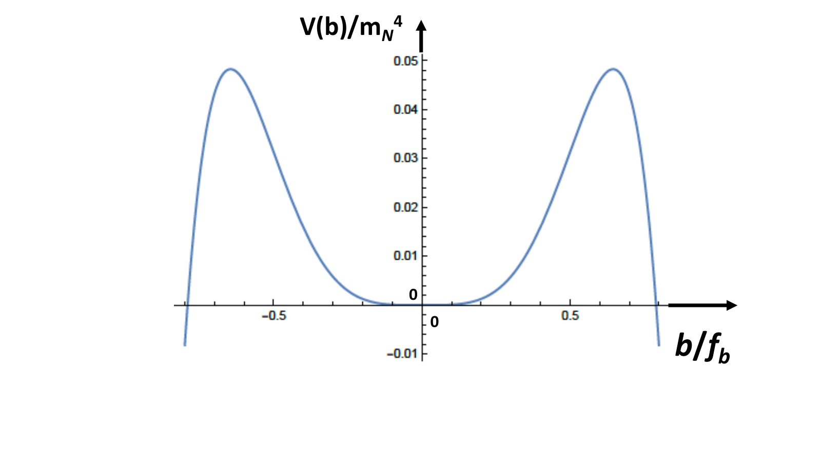
From the Higgs-potential analogue in Branchina and Messina 2013,2020 20 The potential (50) has even powers of the field, hence the pseudoscalar nature of the field is not relevant for our considerations here. The effective potential here resembles the effective potential appearing in the analysis of the (meta)stability of the Higgs vacuum; we follow that analysis in determining the stability of the axion potential. we may rewrite the effective potential (50) for relatively large values of the field , relevant for the metastability argument, as:
| (60) |
Under assumption (56), for values of such that
| (61) |
the effective self-interaction coupling defined in (60) changes sign from positive to negative, thus triggering a potential instability (see fig. 1). In the scheme, in which (55) is valid, the instability arises for values of .
To estimate the false vacuum lifetime, we remark that we write the effective potential in the form (60), and reverse the sign of the coupling Coleman 1977; Callan and Coleman 1977
| (62) |
for a Euclidean scalar theory; there are known bounce solutions, used in the estimation of the tunnelling time of the false vacuum Coleman 1977; Callan and Coleman 1977. Because of (62) and (55) (in the scheme), , the potential (60) of fig. 1 is reversed in sign, thus acquiring a Higgs-like form, where the local unstable maxima at (cf. Fig. 1) correspond (in the Euclidean case) to non-trivial minima:
| (63) |
Then, following Coleman 1977; Callan and Coleman 1977, the (inverse of the) tunnelling time (lifetime) of the false vacuum is computed as:
| (64) |
where denotes the vacuum expectation value that minimises the quartic axion potential, in terms of which the bounce is found: in this case ; (where ) is the Euclidean (E) solution for the bounce; is the action for the bounce; the notation means that the zero-modes are excluded in the computation of the determinant; a a prime over the potential denotes derivative with respect to the axion field ; the quantity denotes the the age of the Universe and is estimated by the cosmological data Aghanim et al. 2020 to be 13.8 billion years, or in reduced Planck-mass units
| (65) |
The boundary between the metastability and instability regions of the axion potential is , with indicating a metastable (unstable) vacuum.
The action of the bounce for the model involving the unstable terms in the potential (60), can be calculated numerically only Branchina and Messina 2013; Branchina et al. 2014, extending standard methods Coleman 1977; Lee and Weinberg 1986, to obtain:
| (66) |
where
| (67) |
and denotes the coupling of the inverted standard scalar potential, , without the corrections, and the coefficient defines the corrections in the (Euclideanised) potential (60), which (on assuming the -scheme condition (55)) we write in the form :
| (68) |
As becomes clear from its form (cf. the inverted analogue of fig. 1), the Euclidean potential (68) can be well approximated with just the inverted potential for . Following the general method of Lee and Weinberg 1986, which was used in Branchina and Messina 2013 to estimate the lifetime of the Higgs (false) vacuum from new physics corrections, it suffices to evaluate the lifetime of the false vacuum associated with the potential (68), and at the point where the bounce , with given by (63).
From (68), (67), we therefore have that at such values of
| (69) |
According to the (numerical) analysis for the existence of bounce solutions performed in Branchina and Messina 2013; Branchina et al. 2014, such solutions do exist, provided , which is satisfied by (69) for our axion system. Indeed, the (approximate) bounce solutions of the Euclidean equations of motion for the -corrected potential are given by Branchina and Messina 2013; Branchina et al. 2014:
where , and , which confirms explicitly our earlier assertion that the bounce solution exists only for Branchina and Messina 2013; Branchina et al. 2014.
The analysis of Branchina and Messina 2013 also shows that there are other approximate bounce solutions for the range of , which are those of the original scalar potential , of the form:
| (72) |
where the size of these bounces can take any value in the range . The Euclidean action of such bounces is independent of and of the form of the standard scalar potential Coleman 1977:2121 21 The degeneracy with respect to the size of the bounce is lifted by considering one-loop corrections, which are calculated on top of the classical solutions, and which select one particular value for the size.
| (73) |
The explicit computation of the determinant factors in (64) for the bounce solution yields the formula for the total width of the false vacuum corresponding to (68) (in the concrete case of, say, two (approximate) bounce solutions , , assumed to have been selected by quantum corrections to the action):
| (74) |
where labels the bounce solutions (IV) and (72), respectively, with sizes , bounce actions in (66), (73), and the loop corrections to the bounce actions. When the axion potential (68) (or, equivalently (60)) is generated at one loop, we set
| (75) |
to avoid overcounting of the quantum corrections.
On taking into account (69), the actions (73) and (66) of the two bounce solutions are of the same order:
| (76) |
This differs from the standard Higgs-potential case Isidori et al. 2001b; Branchina and Messina 2013; Branchina et al. 2014, where the “new-physics” bounce solutions (from powers of the Higgs scalar higher than four), lead to actions that are smaller by several orders of magnitude Branchina and Messina 2013 from the action of the standard bounce. Thus, in our case, such solutions will not affect the order of magnitude of the estimate of the lifetime of the false vacuum based only on the bounce solution (IV). Hence we restrict ourselves only to the bounce , corresponding to (68), in (74), and set the renormalisation group (RG) scale equal to the size of the bounce,
| (77) |
We select to maximise the tunnelling probability Isidori et al. 2001b. Although we have taken the bounce to be the classical Euclidean solution (to the equations of motion corresponding to the effective potential (68) assuming(55)), when calculating the lifetime we take into account one-loop corrections, by using running couplings. Explicitly the couplings in the respective formulae are replaced by the running ones evaluated at the point , with given by (63), while we set the RG scale equal to the bounce size (77) that minimizes the lifetime.
On account of (75), we consider only the bounce in (74), and set . Hence, we evaluate the (minimal) lifetime at a bounce size which maximises the probability of tunnelling of the false vacuum, using the formula:
| (78) |
Here is the running RG scale at the value that minimises the quantity Branchina and Messina 2013; Branchina et al. 2014, which is indicated by the “” symbol in (78).
The running of the with the RG scale requires further analysis if one wishes to include higher-loop corrections to the masses and wave-function renormalization of the KR axion field ; our analysis suffices since we are interested only in the leading estimate of the tunnelling time, compared with .
We observe that, in the case that the effective coupling in (60) is positive (), it increases with the RG scale , since:
| (79) |
on assuming bare quantities for and , i.e. ignoring mass and wave-function renormalization effects to leading order 2222 22 The latter depend on the underlying detailed microscopic model for the KR axion which we ignore in this work..
Let us suppose, for concreteness, (e.g. either generic Einstein-Cartan torsion models (35), or string-inspired models in which ). In such cases, at an initial UV cut-off scale of the effective theory, which can be set to be the heavy RHN mass GeV of the CPTV leptogenesis model of Mølgaard and Shrock 2014, the effective coupling (in the Minkowski-spacetime effective potential) takes on the value:
| (80) |
with the scale being given by (63). Thus, due to (79), becomes smaller as we decrease , until reaches a value for which vanishes, and then becomes negative.
From (78) we then observe formally that when there is no minimum of , unless , in which case, as we observe from (60) and (78), (we assume that the fields , are such that does not vanish). Indeed, for , we have
| (81) |
Thus, passing onto the Euclidean spacetime to compute quantities associated with the lifetime , we have (with the index denoting Euclidean quantities):
| (82) |
On the other hand,
| (83) |
Thus, there is a monotonic decrease of in this case, with the (trivial) minimum occurring for , for which .
Minimisation of , on the other hand, occurs for negative . Indeed it can be readily seen that the mimimum of occurs for such that:
| (84) |
To estimate the in (84) we need to know an estimate of the bounce solution of the effective potential (60). Following Branchina et al. 2014; Lee and Weinberg 1986 we set ((63)) in the estimation of that enters the formula (78) for the computation of the false-vacuum life time. In the full theory, to which the axion system under consideration is embedded, one needs to compute loop corrections to the running , and use such complete expressions in the estimate of the life time using (78).
From (84) we observe that for the CPTV leptogenesis model of Mølgaard and Shrock 2014, for which GeV the minimum , approaching zero for all practical purposes (infrared fixed point). Such minima correspond to very-large-size instantons. In such a regime of , the lifetime of the vacuum (78) can be very large (practically infinite), as follows from the very small value (cf. (84)) of , for which characterises the model of leptogenesis of Mølgaard and Shrock 2014:
| (85) |
In this region of the KR axion acquires a negative mass square, which, in combination with the fact that the entire axion potential (50) is negative in this case, leads to a stable situation in which the KR axion appears as a tachyon matter field with negative unstable potential energy. Such a phase is unphysical, and thus we discard it. Nonetheless, it is worth noting that in our simplified system the tachyon appears as a metastable phase of the leptogenesis model of Mølgaard and Shrock 2014, with a lifetime much longer than the age of the Universe, , provided , which is the case of either Einstein-Cartan torsion theories (35), or large-scale string theories with (13). However, for low string mass scales , for instance, such that (13), we see that the vacuum is highly unstable, with .
On the other hand, for , which is the regime of interest to us, if we want to generate dynamically an axion mass in a regime relevant to DM interpretations of the KR axion, the lifetime of the corresponding false vacuum can be computed from (78) to yield:
| (86) |
where we took into account the age of the Universe (65).2323 23 On the other hand, for very large (transplanckian) field values such that (87) in the right-hand-side of the last equality of (84), we observe that the minimum of occurs within the desired regime (56), in which the one-loop-induced effective mass term of the axion field is a proper mass, and the vacuum is again metastable, given that (we remark that we are agnostic though as to whether such transplanckian field values make sense in an UV complete theory of quantum gravity, such as string theory Ooguri and Vafa 2007; Palti 2019; Garg and Krishnan 2019; Ooguri et al. 2019; Denef et al. 2018; Martin and Brandenberger 2001.) For the cases of generic Einstein-Cartan torsion theories (35), or large-scale string theories ( (13)), this yields clearly a metastable vacuum, with . From (IV), for , for instance, such that (13), we see that the vacuum is highly unstable, with .
It would be interesting to consider the effect of dimension-eight (), or even higher-order, operators in our analysis, and establish whether there is a second local minimum in the corresponding effective potential. (In the example of new physics for the Higgs potential examined in Branchina and Messina 2013; Branchina et al. 2014, and discussed above, this was the case.) We could then find a minimum . Whether such a situation is realised, remains to be seen although we expect this to be the case in view of the analysis in Coleman and Weinberg 1973; Manohar and Nardoni 2021 at one loop for the effective potential. Indeed, that work implies that the subdominant dimension 8 operator gives a positive contribution due to logarithmic corrections to the quartic scalar self-interaction (see footnote 17).
From the above discussion, we conclude that for the regime of parameters of the models we study, one faces a metastable vacuum for the KR axion , with , in string-inspired models with . In view of its acquired mass (57), of for concrete string models (III.1) with , or generic Einstein-Cartan theories (35), the KR axion could play the rôle of an axion-like-particle (ALP) DM component Preskill et al. 1983; Abbott and Sikivie 1983; Dine and Fischler 1983; Marsh 2016, in a range consistent with astrophysical and cosmological constraints Mehta et al. 2020. We remark, though, that, due to (13), the upper bound on the ALP mass is quite restrictive for the string scale in such models, allowing only models with large string mass scales close to (i.e. at most a couple of orders away from) the Planck mass. This is also consistent with the generic Einstein-Cartan torsion models, (35)).
V Conclusions
In this work we have established formally a connection between contorted geometry and particle dark matter by exploiting the role of torsion as axion-like particles in a model for CPTV leptogenesis with heavy RHN. Specifically, we have considered two frameworks in which torsion induced axions develop an effective potential as a result of integrating out these heavy sterile fermions.
- 1.
The first framework is the Einstein-Cartan theory in which the axion couples to massless and massive fermions. The chiral anomalies associated with chiral (massless) fermions imply in such theories a coupling of the geometric axion with gauge and gravitational Chern-Simons terms with a dimensionful coupling constant of the order of the Planck scale.
- 2.
The second framework is a string-inspired gravitational theory, in which the role of torsion is played by the field strength of an antisymmetric tensor spin one field of the massless gravitational multiplet of the string. This behaves as a totally antisymmetric component of the torsion, which in dimensions is dual to an axion like particle, which shares similar couplings to Chern-Simons anomalies to the Einstein-Cartan framework. This framework contains many degrees of freedom that contribute to the phenomenology in addition to the torsion induced axion compared to the first framework.
Using the methods of effective field theory, we find a one-loop quantum potential for our axion at energies low compared to the RHN mass . The potential is negative for large enough values of the field and so the issue of vacuum stability of the axion field arises. We have found that the stability of the axion vacuum depends on the ratio of the axion coupling to , as seen in (IV). It should be stressed that our effective field theory is valid for . We found that for high values of , the vacuum is metastable with a life time much longer than the age of the Universe. In such cases, the axions acquire an effective mass which makes them credible DM candidates. On the other hand, a ratio is not viable for our model, as it leads to very short vacuum life times.
In our approach we have considered for simplicity truncation of the one-loop effective axion potential to dimension six operators. It would be desirable to explore the effective potential to all powers of the axion field, using the methods of Coleman and Weinberg Coleman and Weinberg 1973. We shall also investigate gradient effects in the calculation of the tunnelling rate to the true vacuum Garbrecht and Millington 2015, due to the spatial inhomogeneities of the bounce solution.
Acknowledgments
We acknowledge discussions with Sebastian Ellis, Ken Mimasu and Tevong You. The work of N.E.M. and S.S. is supported in part by the UK Science and Technology Facilities research Council (STFC) and UK Engineering and Physical Sciences Research Council (EPSRC) under the research grants ST/T000759/1 and EP/V002821/1, respectively. N.E.M. also acknowledges participation in the COST Association Action CA18108 “Quantum Gravity Phenomenology in the Multimessenger Approach (QG-MM)”. We thank Carl Bender for a useful discussion.
Appendix A Lifetime estimate using the full potential
We supplement the numerical calculations in Sec.IV with related analysis in which we include the mass terms when finding the maximum of the potential terms (cf. (63)). The method is semi-analytic but this additional refinement does not change any conclusion. We work in terms of the variable where and . In terms of and (where ) the rescaled effective potential Eq(60) is
| (88) |
and the effective quartic coupling in the Euclidean formulation is
| (89) |
The characteristic size of the potential is estimated from the condition
| (90) |
which will also be relevant in the estimation of the lifetime of the KR axion vacuum. In terms of the solution of (90) is where
| (91) |
and
| (92) |
The maximum of occurs for (cf. (63)). Moreover, Pad approximants represent well
| (93) |
where
for small 2424 24 The use of Pad approximants leads to poles for of which all but one are spurious and not in the region of physical interest and so the approximation is useful Bender and Orszag 1978. . .The lifetime of the axion vacuum is approximated by
| (94) |
where . On minimising we find which requires . We recall that the mass scale is used in dimensional regularisation to make the couplings dimensionless. Let us reexamine the scaling properties of the tunnelling (bounce) configuration (for which we do not have an analytic form). The bounce is localised in a spacetime volume of size where and will be denoted by . is small for a bounce and hence there is a contribution from large . The field configuration consists of a wave packet with large . The action for this configuration is
| (95) |
By choosing we would probe strongly the term () which is responsible for tunnelling and this is consistent with the minimising criterion for the lifetime.
References
- Aghanim et al. (2020) N. Aghanim et al. (Planck), Astron. Astrophys. 641, A6 (2020), [Erratum: Astron.Astrophys. 652, C4 (2021)], eprint 1807.06209.
- Streater and Wightman (1989) R. F. Streater and A. S. Wightman, PCT, spin and statistics, and all that (1989), ISBN 978-0-691-07062-9.
- Schwartz (2013) M. D. Schwartz, Quantum Field Theory and the Standard Model (Cambridge University Press, 2013).
- Luders (1957) G. Luders, Annals Phys. 2, 1 (1957).
- Sakharov (1967) A. D. Sakharov, Pisma Zh. Eksp. Teor. Fiz. 5, 32 (1967).
- Bigi and Sanda (2009) I. I. Bigi and A. I. Sanda, CP violation, vol. 9 (Cambridge University Press, 2009), ISBN 978-0-511-57728-4, 978-0-521-84794-0, 978-1-107-42430-2.
- Shaposhnikov (2009) M. Shaposhnikov, Prog. Theor. Phys. 122, 185 (2009).
- Fukugita and Yanagida (1986) M. Fukugita and T. Yanagida, Phys. Lett. B 174, 45 (1986).
- Mohapatra and Pal (1991) R. N. Mohapatra and P. B. Pal, Massive neutrinos in physics and astrophysics, vol. 41 (1991).
- Davidson et al. (2008) S. Davidson, E. Nardi, and Y. Nir, Phys. Rept. 466, 105 (2008), eprint 0802.2962.
- Covi et al. (1996) L. Covi, E. Roulet, and F. Vissani, Phys. Lett. B 384, 169 (1996), eprint hep-ph/9605319.
- Buchmuller et al. (2005a) W. Buchmuller, P. Di Bari, and M. Plumacher, Annals Phys. 315, 305 (2005a), eprint hep-ph/0401240.
- Buchmuller et al. (2005b) W. Buchmuller, R. D. Peccei, and T. Yanagida, Ann. Rev. Nucl. Part. Sci. 55, 311 (2005b), eprint hep-ph/0502169.
- Pilaftsis and Underwood (2004) A. Pilaftsis and T. E. J. Underwood, Nucl. Phys. B 692, 303 (2004), eprint hep-ph/0309342.
- Pilaftsis and Underwood (2005) A. Pilaftsis and T. E. J. Underwood, Phys. Rev. D 72, 113001 (2005), eprint hep-ph/0506107.
- Gorbunov and Rubakov (2011) D. S. Gorbunov and V. A. Rubakov, Introduction to the theory of the early universe: Cosmological perturbations and inflationary theory (2011).
- Luty (1992) M. A. Luty, Phys. Rev. D 45, 455 (1992).
- Mavromatos and Sarkar (2013) N. E. Mavromatos and S. Sarkar, Eur. Phys. J. C 73, 2359 (2013), eprint 1211.0968.
- de Cesare et al. (2015) M. de Cesare, N. E. Mavromatos, and S. Sarkar, Eur. Phys. J. C 75, 514 (2015), eprint 1412.7077.
- Ellis et al. (2013) J. Ellis, N. E. Mavromatos, and S. Sarkar, Phys. Lett. B 725, 407 (2013), eprint 1304.5433.
- Bossingham et al. (2018) T. Bossingham, N. E. Mavromatos, and S. Sarkar, Eur. Phys. J. C 78, 113 (2018), eprint 1712.03312.
- Bossingham et al. (2019) T. Bossingham, N. E. Mavromatos, and S. Sarkar, Eur. Phys. J. C 79, 50 (2019), eprint 1810.13384.
- Mavromatos and Sarkar (2018) N. E. Mavromatos and S. Sarkar, Universe 5, 5 (2018), eprint 1812.00504.
- Mavromatos and Sarkar (2020) N. E. Mavromatos and S. Sarkar, Eur. Phys. J. C 80, 558 (2020), eprint 2004.10628.
- Mavromatos (2022a) N. E. Mavromatos, Phil. Trans. A. Math. Phys. Eng. Sci. 380, 20210188 (2022a), eprint 2108.02152.
- Green et al. (2012a) M. B. Green, J. H. Schwarz, and E. Witten, Superstring Theory Vol. 1: 25th Anniversary Edition, Cambridge Monographs on Mathematical Physics (Cambridge University Press, 2012a), ISBN 978-1-139-53477-2, 978-1-107-02911-8.
- Green et al. (2012b) M. B. Green, J. H. Schwarz, and E. Witten, Superstring Theory Vol. 2: 25th Anniversary Edition, Cambridge Monographs on Mathematical Physics (Cambridge University Press, 2012b), ISBN 978-1-139-53478-9, 978-1-107-02913-2.
- Duncan et al. (1992) M. J. Duncan, N. Kaloper, and K. A. Olive, Nucl. Phys. B 387, 215 (1992).
- Polchinski (2007a) J. Polchinski, String theory. Vol. 1: An introduction to the bosonic string, Cambridge Monographs on Mathematical Physics (Cambridge University Press, 2007a), ISBN 978-0-511-25227-3, 978-0-521-67227-6, 978-0-521-63303-1.
- Polchinski (2007b) J. Polchinski, String theory. Vol. 2: Superstring theory and beyond, Cambridge Monographs on Mathematical Physics (Cambridge University Press, 2007b), ISBN 978-0-511-25228-0, 978-0-521-63304-8, 978-0-521-67228-3.
- Colladay and Kostelecky (1998) D. Colladay and V. A. Kostelecky, Phys. Rev. D 58, 116002 (1998), eprint hep-ph/9809521.
- Kostelecky and Russell (2011) V. A. Kostelecky and N. Russell, Rev. Mod. Phys. 83, 11 (2011), eprint 0801.0287.
- Mavromatos (2014) N. E. Mavromatos, Hyperfine Interact. 228, 7 (2014), eprint 1312.4304.
- Antoniadis et al. (1989) I. Antoniadis, C. Bachas, J. R. Ellis, and D. V. Nanopoulos, Nucl. Phys. B 328, 117 (1989).
- Mølgaard and Shrock (2014) E. Mølgaard and R. Shrock, Phys. Rev. D 89, 105007 (2014), eprint 1403.3058.
- Basilakos et al. (2020a) S. Basilakos, N. E. Mavromatos, and J. Solà Peracaula, Phys. Rev. D 101, 045001 (2020a), eprint 1907.04890.
- Basilakos et al. (2020b) S. Basilakos, N. E. Mavromatos, and J. Solà Peracaula, Phys. Lett. B 803, 135342 (2020b), eprint 2001.03465.
- Mavromatos and Solà Peracaula (2021a) N. E. Mavromatos and J. Solà Peracaula, Eur. Phys. J. ST 230, 2077 (2021a), eprint 2012.07971.
- Mavromatos and Solà Peracaula (2021b) N. E. Mavromatos and J. Solà Peracaula, Eur. Phys. J. Plus 136, 1152 (2021b), eprint 2105.02659.
- Sarkar (2022) S. Sarkar, PoS DISCRETE2020-2021, 039 (2022), eprint 2206.05203.
- Mavromatos (2021) N. E. Mavromatos, Universe 7, 480 (2021), eprint 2111.05675.
- Cartan et al. (2001) É. Cartan, V. V. Goldberg, and S. shen Chern (2001).
- Utiyama (1956) R. Utiyama, Phys. Rev. 101, 1597 (1956).
- Kibble (1961) T. W. B. Kibble, J. Math. Phys. 2, 212 (1961).
- Adler (1969) S. L. Adler, Phys. Rev. 177, 2426 (1969).
- Fujikawa (1979) K. Fujikawa, Phys. Rev. Lett. 42, 1195 (1979).
- Gross and Sloan (1987) D. J. Gross and J. H. Sloan, Nucl. Phys. B 291, 41 (1987).
- Metsaev and Tseytlin (1987) R. R. Metsaev and A. A. Tseytlin, Nucl. Phys. B 293, 385 (1987).
- Bento and Mavromatos (1987) M. C. Bento and N. E. Mavromatos, Phys. Lett. B 190, 105 (1987).
- Kalb and Ramond (1974) M. Kalb and P. Ramond, Phys. Rev. D 9, 2273 (1974).
- Green and Schwarz (1984) M. B. Green and J. H. Schwarz, Phys. Lett. B 149, 117 (1984).
- Gasperini (2013) M. Gasperini, Theory of Gravitational Interactions, Undergraduate Lecture Notes in Physics (Springer Milan, Milano, 2013), 1st ed., ISBN 88-470-2691-1.
- Jackiw and Pi (2003) R. Jackiw and S. Y. Pi, Phys. Rev. D 68, 104012 (2003), eprint gr-qc/0308071.
- Hehl et al. (1976) F. W. Hehl, P. Von Der Heyde, G. D. Kerlick, and J. M. Nester, Rev. Mod. Phys. 48, 393 (1976).
- Shapiro (2002) I. L. Shapiro, Phys. Rept. 357, 113 (2002), eprint hep-th/0103093.
- Svrcek and Witten (2006) P. Svrcek and E. Witten, JHEP 06, 051 (2006), eprint hep-th/0605206.
- Arvanitaki et al. (2010) A. Arvanitaki, S. Dimopoulos, S. Dubovsky, N. Kaloper, and J. March-Russell, Phys. Rev. D 81, 123530 (2010), eprint 0905.4720.
- Marsh (2016) D. J. E. Marsh, Phys. Rept. 643, 1 (2016), eprint 1510.07633.
- Mehta et al. (2021) V. M. Mehta, M. Demirtas, C. Long, D. J. E. Marsh, L. McAllister, and M. J. Stott, JCAP 07, 033 (2021), eprint 2103.06812.
- Mehta et al. (2020) V. M. Mehta, M. Demirtas, C. Long, D. J. E. Marsh, L. Mcallister, and M. J. Stott (2020), eprint 2011.08693.
- Alexander et al. (2006a) S. H.-S. Alexander, M. E. Peskin, and M. M. Sheikh-Jabbari, Phys. Rev. Lett. 96, 081301 (2006a), eprint hep-th/0403069.
- Alexander et al. (2006b) S. H.-S. Alexander, M. E. Peskin, and M. M. Sheikh-Jabbari, eConf C0605151, 0022 (2006b), eprint hep-ph/0701139.
- Lyth et al. (2005) D. H. Lyth, C. Quimbay, and Y. Rodriguez, JHEP 03, 016 (2005), eprint hep-th/0501153.
- Mavromatos (2022b) N. E. Mavromatos, in 740. WE-Heraeus-Seminar: Experimental Tests and Signatures of Modified and Quantum Gravity Workshop (2022b), eprint 2205.07044.
- McAllister et al. (2010) L. McAllister, E. Silverstein, and A. Westphal, Phys. Rev. D 82, 046003 (2010), eprint 0808.0706.
- Silverstein and Westphal (2008) E. Silverstein and A. Westphal, Phys. Rev. D 78, 106003 (2008), eprint 0803.3085.
- Lima et al. (2013) J. A. S. Lima, S. Basilakos, and J. Sola, Mon. Not. Roy. Astron. Soc. 431, 923 (2013), eprint 1209.2802.
- Perico et al. (2013) E. L. D. Perico, J. A. S. Lima, S. Basilakos, and J. Sola, Phys. Rev. D 88, 063531 (2013), eprint 1306.0591.
- Shapiro and Sola (2000) I. L. Shapiro and J. Sola, Phys. Lett. B 475, 236 (2000), eprint hep-ph/9910462.
- Mavromatos and Soto (2021) N. E. Mavromatos and A. Soto, Nucl. Phys. B 962, 115275 (2021), eprint 2006.13616.
- Mavromatos et al. (2022a) N. E. Mavromatos, V. C. Spanos, and I. D. Stamou, Phys. Rev. D 106, 063532 (2022a), eprint 2206.07963.
- Hull (1986) C. M. Hull, Phys. Lett. B 167, 51 (1986).
- Mavromatos (1988) N. E. Mavromatos, J. Phys. A 21, 2279 (1988).
- Preskill et al. (1983) J. Preskill, M. B. Wise, and F. Wilczek, Phys. Lett. B 120, 127 (1983).
- Abbott and Sikivie (1983) L. F. Abbott and P. Sikivie, Phys. Lett. B 120, 133 (1983).
- Dine and Fischler (1983) M. Dine and W. Fischler, Phys. Lett. B 120, 137 (1983).
- Adams et al. (2022) C. B. Adams et al., in Snowmass 2021 (2022), eprint 2203.14923.
- Peccei and Quinn (1977) R. D. Peccei and H. R. Quinn, Phys. Rev. Lett. 38, 1440 (1977).
- Nakahara (1990) M. Nakahara, Geometry, topology and physics, Graduate student series in physics (Hilger, Bristol, 1990), URL https://cds.cern.ch/record/206619.
- Poplawski (2011) N. J. Poplawski, Annalen Phys. 523, 291 (2011), eprint 1005.0893.
- Coleman and Weinberg (1973) S. R. Coleman and E. J. Weinberg, Phys. Rev. D 7, 1888 (1973).
- Manohar and Nardoni (2021) A. V. Manohar and E. Nardoni, JHEP 04, 093 (2021), eprint 2010.15806.
- Burgess (2020) C. P. Burgess, Introduction to Effective Field Theory (Cambridge University Press, 2020), ISBN 978-1-139-04804-0, 978-0-521-19547-8.
- Georgi (1993) H. Georgi, Ann. Rev. Nucl. Part. Sci. 43, 209 (1993).
- Profumo (2017) S. Profumo, An Introduction to Particle Dark Matter (World Scientific, 2017), ISBN 978-1-78634-000-9, 978-1-78634-001-6, 978-1-78634-001-6.
- Dine and Seiberg (1986) M. Dine and N. Seiberg, Nucl. Phys. B 273, 109 (1986).
- Sher (1989) M. Sher, Phys. Rept. 179, 273 (1989).
- Ellis et al. (2020) S. A. R. Ellis, J. Quevillon, P. N. H. Vuong, T. You, and Z. Zhang, JHEP 11, 078 (2020), eprint 2006.16260.
- Zhang (2017) Z. Zhang, JHEP 05, 152 (2017), eprint 1610.00710.
- Mavromatos et al. (2022b) N. E. Mavromatos, S. Sarkar, and A. Soto, Phys. Rev. D 106, 015009 (2022b), eprint 2111.05131.
- Holdom and Peskin (1982) B. Holdom and M. E. Peskin, Nucl. Phys. B 208, 397 (1982).
- Castillo-Felisola et al. (2015) O. Castillo-Felisola, C. Corral, S. Kovalenko, I. Schmidt, and V. E. Lyubovitskij, Phys. Rev. D 91, 085017 (2015), eprint 1502.03694.
- Glendinning (1994) P. Glendinning, Stability, Instability and Chaos: An Introduction to the Theory of Nonlinear Differential Equations, Cambridge Texts in Applied Mathematics (Cambridge University Press, 1994).
- Kaplan (2005) D. B. Kaplan (2005), eprint nucl-th/0510023.
- Einhorn and Jones (2007) M. B. Einhorn and D. R. T. Jones, JHEP 04, 051 (2007), eprint hep-ph/0702295.
- Recami (1986) E. Recami, Rivista del Nuovo Cimento 9:6, 1 (1986).
- Coleman (1977) S. R. Coleman, Phys. Rev. D 15, 2929 (1977), [Erratum: Phys.Rev.D 16, 1248 (1977)].
- Callan and Coleman (1977) C. G. Callan, Jr. and S. R. Coleman, Phys. Rev. D 16, 1762 (1977).
- Lee and Weinberg (1986) K.-M. Lee and E. J. Weinberg, Nucl. Phys. B 267, 181 (1986).
- Isidori et al. (2001a) G. Isidori, G. Ridolfi, and A. Strumia, Nucl. Phys. B 609, 387 (2001a), eprint hep-ph/0104016.
- Branchina and Messina (2013) V. Branchina and E. Messina, Phys. Rev. Lett. 111, 241801 (2013), eprint 1307.5193.
- Branchina et al. (2014) V. Branchina, E. Messina, and A. Platania, JHEP 09, 182 (2014), eprint 1407.4112.
- Isidori et al. (2001b) G. Isidori, G. Ridolfi, and A. Strumia, Nucl. Phys. B 609, 387 (2001b), eprint hep-ph/0104016.
- Ooguri and Vafa (2007) H. Ooguri and C. Vafa, Nucl. Phys. B 766, 21 (2007), eprint hep-th/0605264.
- Palti (2019) E. Palti, Fortsch. Phys. 67, 1900037 (2019), eprint 1903.06239.
- Garg and Krishnan (2019) S. K. Garg and C. Krishnan, JHEP 11, 075 (2019), eprint 1807.05193.
- Ooguri et al. (2019) H. Ooguri, E. Palti, G. Shiu, and C. Vafa, Phys. Lett. B 788, 180 (2019), eprint 1810.05506.
- Denef et al. (2018) F. Denef, A. Hebecker, and T. Wrase, Phys. Rev. D 98, 086004 (2018), eprint 1807.06581.
- Martin and Brandenberger (2001) J. Martin and R. H. Brandenberger, Phys. Rev. D 63, 123501 (2001), eprint hep-th/0005209.
- Garbrecht and Millington (2015) B. Garbrecht and P. Millington, Phys. Rev. D 92, 125022 (2015), URL https://link.aps.org/doi/10.1103/PhysRevD.92.125022.
- Bender and Orszag (1978) C. M. Bender and S. A. Orszag, Advanced Mathematical Methods for Scientists and Engineers (McGraw-Hill, 1978).