BayesMortalityPlus: A package in \proglangR for Bayesian mortality modelling
Lucas M. F. Silva , Luiz F. V. Figueiredo, Viviana G. R. Lobo, Thaís C. O. Fonseca, Mariane, B. Alves
\PlaintitleBayesMortalityPlus: A package in R for Bayesian graduation of mortality modelling
\ShorttitleBayesMortalityPlus: A package in \proglangR for Bayesian graduation of mortality modelling
\AbstractThe BayesMortalityPlus package provides a framework for modelling and predicting mortality data. The package includes tools for
the construction of life tables based on Heligman-Pollard laws, and also on dynamic linear smoothers. Flexibility is available in terms of modelling so that the response variable may be modeled as Poisson, Binomial or Gaussian. If temporal data is available, the package provides a Bayesian implementation for the well-known Lee-Carter model that allows for estimation, projection of mortality over time, and assessment of uncertainty of any linear or nonlinear function of parameters such as life expectancy. Illustrations are considered to show the capability of the proposed package to model mortality data.
\KeywordsMortality graduation, Heligman-Pollard Model, Dynamic linear models, Bayesian Lee-Carter, \proglangR
\PlainkeywordsBayesian mortality graduation, Heligman-Pollard model, Dynamic linear model, Bayesian Lee-Carter model, R
\AddressViviana G. R. Lobo
Departmento de Métodos Estatísticos
and
Laboratório de Matemática Aplicada
Instituto de Matemática
Universidade Federal do Rio de Janeiro
Av. Athos da Silveira Ramos, Centro de Tecnologia, Bloco C, CEP 21941-909.
E-mail:
URL: https://sites.google.com/a/dme.ufrj.br/viviana/
1 Introduction
Models used to characterize mortality data through the Bayesian paradigm have become more popular and called the attention of actuaries, statisticians, and other researchers in recent years. In the actuarial context, it is essential to understand the mortality behaviour so that smoothed death probabilities over ages can be used for pricing life insurance and annuities. From a demographic point of view, this is an essential tool for understanding the changes of patterns in a population. Thus, applying mathematical formulations, such as mortality laws, smoothing models, and improvement techniques is useful to understand the mortality curves of populations or portfolios. Statistical methodologies that consider Bayesian graduation have been more attractive as it allows for the incorporation of prior knowledge through the prior distributions. Besides, graduation is particularly important at advanced ages, for which exposure numbers are small and data are sparse, see Dodd et al. 2018.
Mortality graduation models have become more sophisticated over time. Kimeldorf and Jones 1967 propose the use of mortality smoothing and the constructions of life tables via Bayesian graduation, and Carlin 1992 proposes the use of Markov chain Monte Carlo (MCMC) techniques to fit mortality curves. Dellaportas et al. 2001 suggest estimating the Heligman–Pollard (HP) laws proposed by Heligman and Pollard 1980 using a non-linear logistic and Log-Normal model that accounts for uncertainty in model parameters. Sherris and Njenga 2011 use the Bayesian vector auto-regressive (BVAR) model for the parameters of the HP model by considering temporal evolution of parameters in the HP function. Dodd et al. 2018 and Hilton et al. 2019 provide a methodology for mortality estimation based on generalized additive models (Wood 2006, GAMs - see) at the youngest ages and use a simpler parametric model at older ages that depend on mortality laws well-established in the literature. Packages and functions for fitting mortality curves have been available in \proglangR environment (R Core Team 2020) for several years, through the Comprehensive R Archive Network (CRAN). The \pkgMortalityLaws package exploits optimization methods for fitting a wide range of point estimates for mortality laws (Pascariu 2022). Recently, this package was removed from CRAN repository and old versions can be accessed at https://cran.r-project.org/src/contrib/Archive/MortalityLaws/. The \pkgdemography package developed by Rob J Hyndman et al. 2019 provides functions for demographic analysis, such as life table calculations, fertility rates, and functional data analysis of mortality rates. In the context of Bayesian computation, R packages have been proposed such as the \pkgHPbayes package that provides the eight parameters of the Heligman-Pollard mortality model using a Bayesian Melding procedure with importance sampling (Sharrow 2012). However, the \pkgHPbayes package is no longer available in the \proglangR CRAN repository. Formerly available versions can be obtained from https://cran.r-project.org/src/contrib/Archive/HPbayes/.
The Heligman-Pollard law considers a specific mathematical function to model mortality rates, as a mixture of infant, young adult, and adult survival functions. However, other flexible smoothing approaches could be considered to model mortality, such as splines techniques (Currie et al. 2004; Camarda et al. 2016; Camarda 2019; Tang et al. 2021). In this context, Camarda 2012 proposes a package in \proglangR called \pkgMortalitySmooth, that provides a framework for smoothing count data assumed to be Poisson-distributed in both one- and two-dimensional settings through P-splines. In addition to the proposal of a function in \pkgBayesMortalityPlus to model mortality curves via the Heligman-Pollard law, in this article, we propose a smoother based on dynamic linear models (DLM) (West and Harrison 1997) that is flexible as splines and has an interpretable parameter for controlling smoothness in the mortality graduation across ages. Dynamic linear models are a large class of models with time-varying parameters, useful for modelling time series data. Basically, the proposal is to consider the age of the individuals as an indexer term rather than the evolution over time. More details about the smoothing proposed model are described in Section 3.
Although the Heligman-Pollard model is well-known for forecasting future mortality rates, there are other models that can be taken into account. Among several methods, the Lee-Carter model (Lee and Carter 1992) is a stochastic demographic model that considers temporal dependence in the data, whereas the Heligman-Pollard is a parameterization function for cross-section data. This was a pioneer work in the mortality modelling of a single population over time. The method is based on a factor model with a latent factor varying across time (a state parameter). Several extensions have been proposed to the Lee-Carter model. Li et al. 2004 present an extension of the Lee-Carter model which allows for mortality prediction when the time series is observed in unequal intervals of time. The paper discusses the effects of parameter estimation and prediction uncertainty when the data is limited. The package \pkgdemography, previously mentioned, implements the original Lee-Carter model and other variants presented in Lee and Miller 2001, Booth et al. 2002, and Hyndman and Shahid Ullah 2007. The package \pkgStMoMo developed by Villegas et al. 2018 fits the Lee-Carter model amongst a handful of other mortality models via generalized non-linear models, using the existent \pkggnm \proglangR package (Turner and Firth 2022). From a Bayesian point of view, several papers have dealt with mortality modelling, such as Czado et al. 2005 and Pedroza 2006. In this way, the package \pkgStanMoMo (Barigou and Goffard 2022) models a variety of popular stochastic models with the help of Stan software via \pkgrstan (Stan Development Team 2020). However, it does require some degree of knowledge of Stan tools to perform mortality graduation.
Although several packages to study mortality data are available, there are some issues that our proposed package \pkgBayesMortalityPlus seeks to solve. Firstly, our package provides a user-friendly interface, as well as instructions and simple examples for running each function available for mortality modelling and prediction. The package provides examples from the Human Mortality Database (HMD 2022), and allows the user to supply external data if desired. Moreover, we perform the full Bayesian inference procedure for several smoothing and prediction models: for the HP laws following the specifications described in Dellaportas et al. 2001, the Lee-Carter model, as described by Pedroza 2006 and the Dynamic Linear Model via forward filtering backward sampling (FFBS) recursions with Gibbs sampling, described in Carter and Kohn 1994 and Frühwirth-Schnatter 1994, and proposed here for mortality graduation. This approach makes it possible to simplify the modelling process for the user, as well as provide estimation and credible intervals of parameters and nonlinear functions of model parameters with correct uncertainty measurement, such as probabilities of death, life expectancy, and an easy visualization through graphic tools. We also provide a specific function for closing life tables that is not available in any of the packages mentioned previously. It is based on the article by Dodd et al. 2018 and aims to obtain a more robust fit for advanced adult ages, for which exposures are usually reduced.
In brief, we review the statistical framework underlying the BayesMortalityPlus package and show its ability to model mortality rates via the Heligman-Pollard laws as suggested by Dellaportas et al. 2001, the Dynamic linear model, and the Lee-Carter model via the Bayesian framework. The inference procedure considers the use of Markov chain Monte Carlo techniques to estimate the mortality curve and to perform prediction. The package was coded in \proglangR and is available on CRAN https://cran.r-project.org/package=BayesMortalityPlus. Version 0.1.0 has been considered for this article.
The remaining text is organized as follows. Section 2 presents the Bayesian Heligman-Pollard model, beginning with a brief review of the original Heligman-Pollard law and its properties. The Bayesian inferential and computational procedures based on Monte Carlo Markov chain techniques are addressed. Section 3 presents the Bayesian graduation via Dynamic Linear Model where we propose to model the mortality rates with age-indexes replacing the usual temporal dimension. Section 4 provides tools to the Bayesian graduation through \pkgBayesMortalityPlus package. Section 4.1 shows an illustrative example modelling the mortality curve via the HP model. The functions available in the package are presented and applied to purposes such as computing life expectations, closing life tables using different methods, and producing plots. In Section 4.2, the same example is considered using the Dynamical linear models. Section 5 introduces the Bayesian Lee-Carter model and some functions supplied in the package are employed. Section 6 concludes with a final discussion and some remarks.
2 Bayesian graduation via Heligman-Pollard model
The methods considered in the BayesMortalityPlus package assume that the process of mortality tables graduation is based on a probabilistic approach that allows the computation of point estimates for mortality rates and life expectations, as well as the measurement of the associated uncertainty. We consider the data in a fixed period of time, where denotes the age of the individuals and assumes an integer value, denotes the number of deaths at age and denotes the total exposure of individuals aged . The central mortality rate is defined as (Bowers 1986) and the probability of death as .
An usual approach considered for mortality graduation uses the well-known Heligman-Pollard law (Heligman and Pollard 1980). The HP model is a parametric function that captures the main characteristics of mortality tables, specified in terms of parameters that aim to have a demographic interpretation of the ages’ effect on the mortality rates. It is written as
| (1) |
Equation (1) provides a mathematical formulation that takes into account three terms, each representing a mortality component over the age domain as illustrated in Figure 1. The first term reflects the fall in mortality during the early childhood years through a rapidly declining exponential curve. The second term, similar to the Log-Normal curve, reflects accident mortality for males and accident plus maternal mortality for the female population, being called the accident hump. The last term reflects the near geometric rise in mortality experienced in advanced ages, through the Gompertz exponential formula as described in Heligman and Pollard 1980. Table 1 summarises the interpretation of each term of the HP model.
| Term | Interpretation | Parameters |
|---|---|---|
| Infant mortality |
measures the level of the mortality.
is an age displacement for the mortality of an infant (age 1). measures the decline of the mortality rate throughout childhood. The parametric domain of these three parameters lies on the interval (0, 1) | |
| "Accident hump" | represents the severity, represents the spread and F the location of the "accident hump". These three parameters have the following domains: , and . | |
| Advanced age mortality | represents the base level of senescent mortality while reflects the rate of increase of that mortality. Their respective domains are: and . | |

To estimate the parameters in equation (1) several methods have been proposed. The first method suggested by Heligman and Pollard 1980 considers weighted least squares with weights . This proposal could be problematic due to the over-parameterization of the model and numerical instabilities. Sharrow 2012 considers the Bayesian Melding with Incremental Mixture Importance Sampling techniques implemented in the HPbayes package. Dellaportas et al. 2001 suggest Bayesian inference using the Markov Chain Monte Carlo method to estimate the parameters. For more details on MCMC algorithms see Gamerman and Lopes 2006.
Following the proposal based on Dellaportas et al. 2001, we assume that the death odds are modelled through the Log-Normal distribution and that all individuals of the same age die independently with the same probability and a constant parameter of variation for all ages. Therefore, the model can be written as
| (2) |
where are independent for all age . Equation (2) can be rewritten in a general form as , with being a parametric function. Thus and . Here the Markov chain Monte Carlo techniques require the updating of parameters that depend on the function and the parameter . See Dellaportas et al. 2001 for a more detailed discussion.
Although the proposal in Dellaportas et al. 2001 considers modelling the odds via a log-normal distribution, several papers make other probabilistic assumptions about the mortality law (Czado et al. 2005, Renshaw et al. 1996, Li 2013). In particular, we are interested in allowing the exposure to be related to the model uncertainty since lower exposure is usually associated with higher variability in the data. Therefore we consider modelling the mortality via Poisson and Binomial models as suggested by Dellaportas et al. 2001.
The Binomial model assumes that , which denotes the death count at age , follows a Binomial distribution with the size parameter being the exposure in age , that is, , with death probability at age given by . On the other hand, the Poisson model considers that represents the death counts for the age following a Poisson distribution with rate for each age. In this case, the exposure is an offset. For these two sampling distributions, we will consider an alternative representation for the HP curve by adding an extra parameter as follows
| (3) |
where the parameter is considered in order to allow for changes in the concavity of the curve at its final portion, resulting in a more flexible approach for capturing mortality trends at advanced ages. These alternative formulations have the advantage that the uncertainty relative to the mortality data changes according to the exposure at each age.
In \pkgBayesMortalityPlus package, the user can estimate the parameters of the HP curve through the function \codehp for the Log-Normal, Binomial, and Poisson models. \pkgBayesMortalityPlus can be installed with the code: {CodeChunk} {CodeInput} R> install.packages("BayesMortalityPlus") The package is loaded within \proglangR as follows: {CodeChunk} {CodeInput} R> library("BayesMortalityPlus") The function reproduces the inference procedure presented by Dellaportas et al. 2001 as follows {Code} hp(x, Ex, Dx, model = c("binomial", "lognormal", "poisson"), M = 50000, bn = round(M/5), thin = 10, m = rep(NA, 8), v = rep(NA, 8), inits = NULL, K = NULL, sigma2 = NULL, prop.control = NULL, reduced_model = FALSE)
- •
The arguments \codex, \codeEx, and \codeDx represent the vector of the ages, exposures by age, and deaths by age, respectively.
- •
The argument \codemodel defines the mortality model chosen by the user. Setting \codemodel = "poisson" assumes that deaths follow the Poisson distribution, setting \codemodel = "binomial" assumes that deaths follow the Binomial distribution, and setting \codemodel = "lognormal" assumes that the odds follow the Log-Normal distribution.
- •
The arguments \codem and \codev can be used to specify means and variances, respectively, for the prior distributions of each parameter, with \codeinits specifying the initial values for the parameters in the algorithm. The \codeK argument specifies the extra parameter for the Binomial and the Poisson models, while \codesigma2 is responsible for the initial value for the variance estimated for the Log-Normal distribution. Also, the argument \codeprop.control tunes the acceptance rate of the MCMC algorithm, for which \codeM iterations are assumed, with burn-in period \codenb and thinning given by the argument \codethin. Details on the specification of the MCMC algorithm can be seen in Gamerman and Lopes 2006.
- •
The argument \codereduced_model allows the user to fit a truncated version of the HP curve, which will be discussed in Section 4.1
The package makes the posterior distribution samples available for the user to make inferences about any transformations of the parameters. Therefore, it is simple to obtain the probability of death for any age . Furthermore, the user is able to compute predictive intervals for and survival probabilities , which can be used to quantify the life expectancy for any required age.
For the Binomial and the Poisson models, the HP formula provides estimates for the central mortality rate . Then, under the assumption of uniform distribution for the deaths over an age interval , we can compute the death probability at age through the usual relation . For the Log-Normal model, these probabilities can be obtained through , where denotes the HP curve at age . Finally, we obtain the point estimation for the death probabilities through the posterior median distribution of .
3 Bayesian graduation via Dynamic Linear Model
Dynamic Linear Models (DLM) (West and Harrison 1997) are usually applied in time series analysis, in order to address intrinsically auto-correlated observations gathered through times . In this work, we adopt a particular specification of the DLM class to produce graduated mortality tables, formally recognising the association between mortality rates for neighbouring ages (or age groups) and imposing smoothness of the estimated mortality curve in the transition between ages. The use of DLMs in mortality studies has been common practice in modelling temporal dependence and has been used for mortality predictions. For instance, the well-known Lee-Carter model (Lee and Carter 1992) considers a dynamical model to estimate temporal improvement for each age and can be used for predicting mortality in future years. Other proposals are Li et al. 2004 and Neves and Migon 2007. The point to be highlighted here is that in our approach dynamic components are indexed by ages and not by time periods, aiming to obtain smooth non-linear graduated curves through ages, as well as to address the autocorrelation among ages. Let and , respectively, denote the death counts and exposure at age and define . We consider a second-order polynomial DLM, as follows:
| (4) | |||||
| (5) | |||||
| (6) |
with random errors , and assumed mutually and sequentially independent. The state denotes the dynamic level of the log mortality, with stochastic evolution guided by equation (5), and controls the level variation between consecutive ages (local slope of the mortality curve), allowing for different gradients through ages since evolves according to the random walk described in equation (6). The smoothness of the graduated mortality curves strongly depends on the magnitude of the evolutional errors’ variances, and , which are specified via discounting strategies, as discussed in West and Harrison 1997.
The model may be rewritten, in the general DLM form, as
where denotes a bivariate Gaussian density and
Details on general forms of the DLMs and specially on the particular case of polynomial trend models, adopted here, are found in West and Harrison 1997 and Petris et al. 2009. A first-order polynomial model, that is, a model with only a dynamic could be able to capture several dynamic mortality patterns over the ages, but the resulting point predictive function for the following ages would be a constant function of . The use of the additional parameter results in a DLM that generates a predictive curve for future ages given by a non-zero slope straight line, thus capturing the increasing mortality risk for advanced ages. The concern with the form of the predictive function associated with the adopted model is justified by the fact that, for advanced ages, it is usual that the databases present a shortage of exposure. Therefore the mortality tables are typically adjusted using information up to a certain age and from that point on, extrapolations are necessary. In \pkgBayesMortalityPlus, the predictive function of the second-order polynomial DLM is used in the extrapolation process of the mortality curve.
The user can estimate the parameters of the DLM through the function \codedlm. The function implements the inference procedure based on West and Harrison 1997 via Gibbs sampling for state space models presented by Carter and Kohn 1994 and Frühwirth-Schnatter 1994 as follows {Code} dlm(y, Ft = matrix(c(1,0), nrow = 1), Gt = matrix(c(1,0,1,1), 2), delta = 0.85, prior = list(m0 = rep(0, nrow(Gt)), C0 = diag(100, nrow(Gt))), prior.sig2 = list(a = 0.01, b = 0.01), M = 5000, bn = 3000, thin = 1, ages = 0:(length(y)-1))
- •
\code
y represents the vector of log mortality rates.
- •
The arguments \codeFt, \codeGt and \codedelta represent the structural elements for the specification of the observational and system equations, and the discount factor (default =0.85) for the smoothing, respectively.
- •
The arguments \codeprior and \codeprior.sig2 can be used to specify prior information, both as a \codelist object. Argument \codeprior receives the prior mean vector and covariance matrix and \codeprior.sig2 receives the prior parameters of the Inverse Gamma distribution for the estimated variance of the process.
- •
The argument \codeages allows the user to define the vector of ages associated with \codey in case the age interval does not equal the default graduation \code0:(length(y)-1).
Samples from the posterior distribution are available for inference about quantities of interest such as the probabilities of death , the associated predictive intervals, and the survival probabilities .
For the DLM approach, the model fit provides samples of the posterior distribution of , from which a point estimate of the log mortality rate can be computed. Since posterior samples are available, the death probability at age can be obtained through the relation . For instance, the posterior median of can be used as the point estimation for the death probabilities.
4 Static graduation with BayesMortalityPlus
In this Section, we present the functions available in \pkgBayesMortalityPlus that can be used in the construction of life tables based on the Heligman-Pollard law and the Dynamic Linear models, respectively, as described in Sections 2 and 3. The main functions for smoothing are \codehp and \codedlm. We also explore the posterior summaries and methodologies for extrapolation. Data from the United States and Portugal, which are extracted from the Human Mortality Database (HMD 2022), are contained in the object \codedata, stratified by sex (as well as total population).
In the following, we present the Bayesian graduation by selecting the total population from the United States over the past forty years. We estimate the mortality curves for the specific years 1980, 1990, 2000, 2010, 2019:
R> library(BayesMortalityPlus) R> data(USA) We load the \pkgdplyr package to extract information from the database in a simple way through the command \codefilter (Wickham et al. 2022, see more details in). Notice that other ways to manipulate the data could be applied. In this example, the vector \code[1:81] means that the ages are selected, so that the exposures () and death counts () for the years considered in the study are specified and filtered up to 80 years old for model fitting. {CodeChunk} {CodeInput} R> ex_1980 <- dplyr::filter(USA, Year == 1980)Dx.Total[1:81] R> ex_1990 <- dplyr::filter(USA, Year == 1990)Dx.Total[1:81] R> ex_2000 <- dplyr::filter(USA, Year == 2000)Dx.Total[1:81] R> ex_2010 <- dplyr::filter(USA, Year == 2010)Dx.Total[1:81] R> ex_2019 <- dplyr::filter(USA, Year == 2019)Dx.Total[1:81]

Figure 2 illustrates the raw mortality rates () over years via command \codeggplot available on \pkggglplot package with the following code: {CodeChunk} {CodeInput} R> qx_1980 <- dx_1980/ex_1980 R> qx_1990 <- dx_1990/ex_1990 R> qx_2000 <- dx_2000/ex_2000 R> qx_2010 <- dx_2010/ex_2010 R> qx_2019 <- dx_2019/ex_2019 R> data = data.frame(idade = 0:80, qx_1980 = qx_1980, qx_1990 = qx_1990, qx_2000 = qx_2000, qx_2010 = qx_2010, qx_2019 = qx_2019) R> data = as.data.frame(data) R> ggplot(data) + scale_y_continuous(trans = "log10", breaks = 10^-seq(0,5), limits = 10^-c(5,0), labels = scales::comma) + scale_x_continuous(breaks = seq(0, 100, by = 10)) + theme_bw() + theme(legend.position = "bottom") + labs(x = "Age", y = "Raw Mortality Rate", title = NULL) + geom_point(aes(x = idade, y = qx_1980, col = "1")) + geom_point(aes(x = idade, y = qx_1990, col = ’2’)) + geom_point(aes(x = idade, y = qx_2000, col = "3")) + geom_point(aes(x = idade, y = qx_2010, col = "4")) + geom_point(aes(x = idade, y = qx_2019, col = "5")) + scale_color_manual(name = NULL, values = c(rainbow(5)), label = c("USA 1980", "USA 1990", "USA 2000", "USA 2010","USA 2019"))
4.1 Heligman-Pollard model
The function \codehp returns an object of class \code"HP", which is an HP curve fit to the input data settled by the user. In this illustration, we consider vague or non-informative prior distributions. Notice that the user could provide their own prior information if desired. The MCMC scheme is the default one. The HP model under a Log-Normal setting for the respective years can be defined using the following code: {CodeChunk} {CodeInput} R> fit_1980 <- hp(0:80, ex_1980, dx_1980, model = "lognormal") Simulating [===================================] 100R> fit_1990 <- hp(0:80, ex_1990, dx_1990, model = "lognormal") Simulating [===================================] 100R> fit_2000 <- hp(0:80, ex_2000, dx_2000, model = "lognormal") Simulating [===================================] 100R> fit_2010 <- hp(0:80, ex_2010, dx_2010, model = "lognormal") Simulating [===================================] 100R> fit_2019 <- hp(0:80, ex_2019, dx_2019, model = "lognormal") Simulating [===================================] 100 The \codesummary function in \proglangR provides a summary table with the estimation of the parameters and the acceptance rate of the MCMC algorithm. As an example, the posterior summary for the 1980-year fit is available using the code: {CodeChunk} {CodeInput} R> summary(fit_1980) mean sd 2.5A 0.001027 0.000053 0.000929 0.001024 0.001134 22.3 B 0.026701 0.006329 0.016337 0.025984 0.040566 22.3 C 0.125931 0.005250 0.115776 0.125809 0.136760 22.3 D 0.000923 0.000031 0.000864 0.000923 0.000987 22.3 E 11.499650 0.697406 10.202269 11.493265 12.926974 22.3 F 21.088628 0.155102 20.791117 21.085325 21.403002 22.3 G 0.000074 0.000003 0.000069 0.000074 0.000079 22.3 H 1.090734 0.000677 1.089432 1.090735 1.092063 22.3 The \codefitted function can provide a summary with the point estimate of death probabilities generated by the model for specific ages: {Code} fitted(fit, age = NULL) The argument \codefit is a fitted curve by the \codehp function via \pkgBayesMortalityPlus package, and the argument \codeage represents the age interval in which the estimation of the death probabilities is desired. The default age interval is set to \codeNULL, which means that the function will return the whole age interval fitted by the model. For illustration, consider setting the ages \code0,20,40,60,80 and the year 1980. {CodeChunk} {CodeInput} R> fitted(fit_1980, age = c(0,20,40,60,80)) age qx_fitted 1 0 0.012809519 2 20 0.001354225 3 40 0.002402713 4 60 0.013353342 5 80 0.071351681
| US 1980 | US 1990 | US 2000 | US 2010 | US 2019 | |
|---|---|---|---|---|---|
| 0.00103 | 0.00077 | 0.00054 | 0.00051 | 0.0004 | |
| (0.00093; 0.00113) | (0.00065; 0.00091) | (0.00048; 0.00062) | (0.00041; 0.00063) | (0.00033; 0.00048) | |
| 0.0267 | 0.0381 | 0.0538 | 0.0901 | 0.0557 | |
| (0.0163; 0.0406) | (0.0171; 0.0697) | (0.0324; 0.0798) | (0.048; 0.1477) | (0.0251; 0.1) | |
| 0.1259 | 0.1328 | 0.1432 | 0.1648 | 0.141 | |
| (0.1158; 0.1368) | (0.1157; 0.1511) | (0.1289; 0.1583) | (0.1429; 0.1895) | (0.1186; 0.1656) | |
| 0.00092 | 0.00077 | 0.0006 | 0.00058 | 0.0008 | |
| (0.00086; 0.00098) | (0.0007; 0.00085) | (0.00056; 0.00065) | (0.00053; 0.00065) | (0.00073; 0.00089) | |
| 11.49 | 6.43 | 11.81 | 8.79 | 4.45 | |
| (10.2; 12.92) | (5.21; 7.98) | (9.93; 13.78) | (7.1; 10.9) | (3.61; 5.43) | |
| 21.08 | 22.8 | 20.9 | 23.7 | 29 | |
| (20.79; 21.4) | (21.97; 23.81) | (20.54; 21.36) | (22.96; 24.57) | (27.54; 30.77) | |
| 0.00007 | 0.00006 | 0.00006 | 0.00005 | 0.00004 | |
| (0.00007; 0.00008) | (0.00005; 0.00007) | (0.00005; 0.00006) | (0.00004; 0.00005) | (0.00003; 0.00005) | |
| 1.091 | 1.091 | 1.090 | 1.091 | 1.091 | |
| (1.0895; 1.0921) | (1.0887; 1.0939) | (1.0889; 1.0915) | (1.0892; 1.0929) | (1.0893; 1.0944) |
One way to evaluate the behaviour of mortality for the United States population over the years and ages is by analysing the estimate of the HP parameters for the five years selected, as shown in Table 2. \pkgBayesMortalityPlus provides tools to check the convergence of the generated Markov chains obtained in the estimation procedure (for more details, see \codeplot_chain). To investigate the mortality improvement over five years, we consider assessing the significance of the parameters through the credible intervals criterion. We consider that there is a significant difference when the credible intervals are disjoint. Notice that parameter decreases significantly from 1980 to 1990 and from 1990 to 2000, and then there is no significant difference, but the point estimate continues to decline. Parameters and show similar interpretations as parameter , both increasing over time until 2010, but in 2019 their estimates decrease to values close to the ones in 2000. It indicates that the changes are not statistically significant in a shorter temporal window. In summary, the level of mortality in the first years of life decreased significantly over the years, except for the last year of the analysis.
For the second term of the Heligman-Pollard law, see that parameter decreases significantly over the years up to 2000, analogous to the estimates of parameter . In 2019, there is a significant increase in its estimate. That means that the level of mortality in the accident hump decreased until 2000, persisted in this level in 2010, and increased in 2019. Parameter indicates that 1980 and 2000 were the years in which the mortality in the accident hump was most severe. The estimate of parameter is around 21 to 24 years until 2010 and in 2019 its estimate becomes almost 29 years, indicating a large shift of the accident hump to older ages. For the last term of the HP function, parameter shows a decreasing behaviour over the years, which means that the level of mortality in adulthood is decreasing over the years. This reduction was significant in the period from 2000 to 2010. On the other hand, parameter remains almost constant in all fits.
To facilitate comparison among the five fitted models, we access the function \codeplot available on \proglangR to visualize the behaviour of the mortality curves. Figure 3 shows the fitted mortality curves for the United States population. {CodeChunk} {CodeInput} R> fits <- list(fit_1980,fit_1990,fit_2000,fit_2010,fit_2019) R> labels <- c("US 1980","US 1990","US 2000","US 2010", "US 2019") R> plot(fits, labels = labels, plotData = F, plotIC = F)

As seen in Figure 3, there is a similar behaviour of the adjusted tables in the first four years of the analysis, except for some level changes that occur between 1980 and 1990 in ages and and also between 2000 and 2010, in ages and . This indicates consistency in the mortality pattern in the US population until 2010. On the other hand, this pattern is missed in 2019, where it can be observed that the accident hump is longer than in previous years, indicating that the causes of death that make up the accident hump are lasting longer than they used to.
Predictive Credible Interval for the probability of death
Function \codeqx_ci computes the predictive credible interval for from \codehp and \codedlm objects via the composition sampling technique (Banerjee et al. 2004, see Chapter 5 of). The following code provides credible intervals based on the HP fit for the year 1980: {CodeChunk} {CodeInput} R> head(qx_ci(fit_1980, age= 1:81, Ex= NULL, prob=0.95)) age qi qs 1 1 0.0009389319 0.0012430310 2 2 0.0005547195 0.0007122412 3 3 0.0004101589 0.0005214704 4 4 0.0003343556 0.0004244586 5 5 0.0002953454 0.0003724304 6 6 0.0002702347 0.0003420523 Arguments \codefit and \codeage are the same as defined in function \codefitted. Parameter \codeEx is a vector of the exposures that is used when the Binomial and Poisson models are fitted since both depend on these quantities. By default, \codeage and \codeEx are set to be the ones passed in the fitting function. If any age outside of those used in the fitted curve is specified, the exposure for that age must also be determined by the user. This is not applied when the Log-Normal model is fitted. Additionally, the user can specify the probability of the predictive credible interval through the argument \codeprob. Figure 4 presents the fitted mortality curve with the 95% predictive credible interval. Figure 4 was obtained with the code: {CodeChunk} {CodeInput} R> plot(fit_1980, labels = "US 1980", plotIC = T, plotData = T)

Life Expectancy
The estimate of life expectancy is obtained via function \codeexpectancy through the curtate life expectancy as follows
| (7) |
where is the maximum age available in the life table, and is the probability that someone aged will attain age . Under the assumption of age-independent mortality, we can write as a cumulative product in terms of the survival probability . Then,
| (8) |
The function is called in thee package as follows: {Code} expectancy(fit, Ex = NULL, age = NULL, graph = TRUE, max_age = 110, prob = 0.95) The output from function \codeexpectancy is an object of the class \codehp and \codedlm, and its arguments are:
- •
\code
fit represents the fitted curve by Heligman-Pollard or Dynamic Linear Model.
- •
Arguments \codeEx and \codeprob are exposure and probability, necessary to calculate the predictive intervals for the expectancy.
- •
By default, \codeEx is set to \codeNULL which indicates that the exposure available for the life expectancy is the same as used in the fitted curve. It is important to note that argument \codeEx is used by the HP Binomial and HP Poisson models to associate the uncertainty with the ammount of available information.
- •
Argument \codemax_age (default=110) represents the maximum age to calculate the life expectancy. If necessary, the \codeexpectancy() function will extrapolate the fitted HP curve until it reaches the maximum age argument. In these cases, it is important to attend to \codeEx argument: if it is set to \codeNULL, the function will repeat the last informed exposure to match the age interval.
The user can obtain the residual life expectancy for specific ages, with age 0 meaning life expectancy at birth. For illustration, consider setting the ages \code0,20,40,60,80 and year 1980, with the following code: {CodeChunk} {CodeInput} R> expectancy(fit_1980, age = c(0,20,40,60,80), graph = F) Age Expectancy Lower CI Upper CI 1 0 73.31 71.77 74.82 21 20 54.91 53.58 56.24 41 40 36.26 35.05 37.47 61 60 19.42 18.44 20.41 81 80 7.51 6.94 8.11 Table 3 presents a summary of the posterior life expectancy for the five models and Figure 5 illustrates the behaviour of the posterior distribution for the life expectancy for selected years. For all ages, we see an increase in life expectancy. Notice that the increase is not significant in close years but is remarkable when the decades are considered. In 2019, the life expectancy at birth is superior by more than five years to that in 1980. In terms of a point estimates, the most considerable difference occurs between 2000 and 2010, while the smallest difference is between 2010 and 2019.
In addition, \pkgBayesMortalityPlus package allows graphical visualization of the behaviour of life expectancy over the years. In Figure 5, we can see stronger blue tones at the bottom for the first ages throughout the years, which represents a larger life expectancy at birth. It is also noticeable that the ages with lightest tones are associated with a life expectancy close to 40 years, and have a slight increase over the years. Because in older ages the life expectancy is small and therefore becomes close for all years, there is no significant change at the top of the graphic.
| Age | US 1980 | US 1990 | US 2000 | US 2010 | US 2019 |
|---|---|---|---|---|---|
| 0 | 73.1 | 75.01 | 76.82 | 78.81 | 79.05 |
| (71.76; 74.82) | (72.75; 77.24) | (75.23; 78.40) | (76.53; 81.04) | (76.89; 81.21) | |
| 10 | 64.54 | 65.97 | 67.54 | 69.42 | 69.61 |
| (63.17; 65.90) | (63.9; 68.03) | (66.05; 69.01) | (67.29; 71.54) | (67.57; 71.67) | |
| 20 | 54.91 | 56.28 | 57.80 | 59.62 | 59.81 |
| (53.57; 56.24) | (54.27; 58.31) | (56.35; 59.25) | (57.52; 61.71) | (57.8; 61.84) | |
| 30 | 45.59 | 46.94 | 48.30 | 50.14 | 50.39 |
| (44.32; 46.86) | (45.02; 48.87) | (46.91; 49.70) | (48.12; 52.15) | (48.47; 52.35) | |
| 40 | 36.26 | 37.62 | 38.85 | 40.68 | 41.14 |
| (35.04; 37.47) | (35.79; 39.47) | (37.51; 40.20) | (38.74; 42.62) | (39.31; 43) | |
| 50 | 27.41 | 28.68 | 29.83 | 31.54 | 32.08 |
| (26.28; 28.54) | (26.99; 30.41) | (28.58; 31.10) | (29.72; 33.39) | (30.37; 33.84) | |
| 60 | 19.42 | 20.52 | 21.57 | 23.09 | 23.59 |
| (18.43; 20.41) | (19.03; 22.07) | (20.46; 22.72) | (21.45; 24.77) | (22.05; 25.20) | |
| 70 | 12.67 | 13.55 | 14.45 | 15.69 | 16.11 |
| (11.87; 13.48) | (12.33; 14.85) | (13.52; 15.41) | (14.32; 17.12) | (14.8; 17.48) | |
| 80 | 7.51 | 8.14 | 8.83 | 9.74 | 10.04 |
| (6.93; 8.1) | (7.23; 9.12) | (8.13; 9.55) | (8.69; 10.85) | (9.03; 11.12) |
R> Heatmap(fits, x_lab = labels, age = 0:80)

Modelling adult ages
Assume a scenario in which interest lies in modelling only the mortality rate for adults. Some issues could result in this scenario such as poor quality of the data on the mortality of infants and young ages or their non-existence. For example, consider an insurance life product for employees of a company. In this case, we would not access data for children and young people due to the fact that they are not legally allowed to work. In this case, the younger ages are not modelled as the first term of the HP curve is not available for analysis. The argument \codereduced_model is available in function \codehp to deal with such situations. For illustration, consider the data for the year 2010 from age 18 (see Figure 6). {CodeChunk} {CodeInput} R> hp.fit2 <- hp(x = 18:80, Ex = ex_2010[19:81], Dx = dx_2010[19:81], model = "lognormal", reduced_model = TRUE) R> plot(hp.fit2, plotIC = F, labels = "HP fitted")

This approach allows fast computations and convergence in the MCMC algorithm for two reasons. Firstly, the dimension of the parameters is reduced, the acceptance rate raises and consequently, the algorithm converges fast. Furthermore, identifiability issues in the parameters , and could occur if they are taken into account in the inference procedure. These parameters are not estimated when considering the \codereduce_model argument.
Mortality measurement at advanced ages and extrapolation
The life tables are composed of the mortality probability , associated with each age . The estimates of mortality at advanced ages are difficult to compute due to the fact that there is a small number of survivors in this age group. In this context, to achieve a robust fit at advanced ages, following Hustead 2005 we consider four methodologies to accommodate the mortality pattern at the end of the mortality graduation. The synopsis of the function \codehp_close is given by: {Code} hp_close(fit, method = c("hp", "plateau", "linear", "gompertz"), x0 = max(fitx), max_age = 120, k = 7, weights = seq(from = 0, to = 1, length.out = 2*k+1), new_Ex = NULL, new_Dx = NULL) This function receives an object of the class \code"HP" adjusted by the function \codehp and fits a closing method to expand the data of the life table to a maximum age argument \codemax_age (default=120) inputted by the user. The user can adopt alternative approaches for closing tables using the argument \codemethod. The package provides four closing methods: \codemethod="hp", \codemethod="plateau", \codemethod="linear" and \codemethod="gompertz". Notice that \codemethod= "linear" can only be used with HP objects following \codemodel="lognormal" option of the HP model. Also,
- •
\code
x0, \codek and \codeweights arguments control the mixture of the fitted HP model to the closing model, representing the starting age for the closing method, the size of the age interval to be mixed and the weights to be applied to the mixture, respectively.
- •
\code
new_Ex and \codenew_Dx arguments represent the data that was not fitted by the original HP curve, the exposure, and the death count after the \codex0 argument. These arguments must be the same length and are required for the Binomial and Poisson mortality models, and also for \codemethod="linear" and \codemethod="gompertz".
For illustration of the closing methods available in \pkgBayesMortalityPlus package, we consider the object \codefit_2019 and age 80-100 (extrapolation).
1. The HP method
The argument \codemethod="hp" extrapolates the fitted Heligman and Pollard 1980 curve to the \codemax_age argument informed by the user. We expect the mean of the posterior distribution to be similar to the values obtained by the \codefitted function, as well as the predictive intervals obtained by the \codeqx_ci function. Since it is just an extrapolation of the HP curve, the mixture is not applied.
{CodeChunk}
{CodeInput}
R> hp.close1 <- hp_close(fit_2019, method="hp", max_age = 100)
2. The Plateau method
The \codemethod= "plateau" considers that the death probability of the last age fitted by the HP model is kept constant until it reaches the maximum age. No mixture is applied. More detailed discussion about this mortality pattern at the oldest ages can be seen in Lai 2012.
{CodeChunk}
{CodeInput}
R> hp.close2 <- hp_close(fit_2019, method="plateau", max_age = 100)
3. The Linear method
The \codemethod="linear" is only available for the Log-Normal model. This method fits a linear regression starting at age until the last age with available data and is specified as:
| (9) | |||
After fitting the linear regression, predictive samples are generated for the death probabilities starting at age , dividing the graduation into three parts: the first one is the fitted curve given by the HP model, followed by the mixture interval given by the \codek argument, ending with the fitted linear regression.
{CodeChunk}
{CodeInput}
R> new_Ex <- dplyr::filter(USA, Year == 2019)Dx.Total[81:101]
R> hp.close3 <- hp_close(fit_2019, method="linear", max_age = 100,
new_Ex = new_Ex, new_Dx = new_Dx)
4. The Gompertz method
Details about the \codemethod="gompertz" are available in Dodd et al. 2018 and Gavrilov and Gavrilova 2011. Dodd et al. 2018 consider the Gompertz curve to close the English life tables between 2010-2012 and conclude that the better the quality of mortality data at advanced ages, the more the behaviour of the mortality curve approaches the Gompertz function.
This method fits the Gompertz curve developed by Gompertz 1825 through the Sampling Importance Resampling method (SIR) as
| (10) | |||
where represents the mortality force that grows exponentially with the increase of age , depending on parameters and . Parameter reflects the general level of mortality, while controls the rate at which the force of mortality increases with age. Notice that if we assume , then that is equivalent to the third term of the eight-parameter HP curve previously seen in Section 2. The results of the Gompertz method are plotted in Figure 7 with 95% predictive credible interval, for the year 2019. Analogously, we can plot the mortality curve and expectancy life for the objects \codefit_hp, \codefit_plat, and \codefit_lin, respectively. {CodeChunk} {CodeInput} R> hp.close4 <- hp_close(fit_2019, method="gompertz", max_age = 100, new_Ex = new_Ex, new_Dx = new_Dx) R> plot(hp.close4, labels = "Gompertz method")

After choosing the closing method, an \code‘ClosedHP’ object will be generated to save the new life table. This allows the new complete graduation to be used as an argument to other functions in the package. For example, in Figure 8 the life expectancy is shown and compared with different closing methods via object \codefits.new. {CodeChunk} {CodeInput} R> fits.new <- list(hp.close1, hp.close2, hp.close3, hp.close4) R> Heatmap(fits.new, x_lab = c("HP","Plateau","Linear","Gompertz"))

4.2 Mortality Graduation via Dynamical Linear Smoothers
The function \codedlm returns an object of class \code"DLM", which is a Dynamic linear model with input data settled by the user. We consider the same dataset for which we have applied the Heligman-Pollard model, with the data being transformed into log mortality to reproduce the results of the graduation mortality curves. To fit a dynamical linear model under the log mortality for five different years, consider the following code: {CodeChunk} {CodeInput} R> y_1980 <- log(dx_1980/ex_1980) R> y_1990 <- log(dx_1990/ex_1990) R> y_2000 <- log(dx_2000/ex_2000) R> y_2010 <- log(dx_2010/ex_2010) R> y_2019 <- log(dx_2019/ex_2019)
R> dlm_1980 <- dlm(y_1980, delta=0.85) Simulating [===================================] 100R> dlm_1990 <- dlm(y_1990, delta=0.85) Simulating [===================================] 100R> dlm_2000 <- dlm(y_2000, delta=0.85) Simulating [===================================] 100R> dlm_2010 <- dlm(y_2010, delta=0.85) Simulating [===================================] 100R> dlm_2019 <- dlm(y_2019, delta=0.85) Simulating [===================================] 100 Posterior summaries for the five fitted models are allowed via the \codesummary function available in \codeR. For illustration, we exhibit posterior summaries for the year 1980 and some ages, as follows: {CodeChunk} {CodeInput} R> head(summary(dlm_1980))
mean sd 2.5sigma2 0.00932 0.00203 0.00594 0.00910 0.01380 mu[0] -4.35763 0.09607 -4.55490 -4.35698 -4.15945 mu[1] -6.92630 0.09633 -7.11315 -6.92766 -6.74431 mu[2] -7.32963 0.09376 -7.52254 -7.32660 -7.14864 mu[3] -7.60248 0.09030 -7.78687 -7.60194 -7.43082 mu[4] -7.86710 0.07516 -8.01933 -7.86680 -7.71978 Note that \codemu[] represents the posterior mean of the log mortality rate for each age in the study. The user can also call the \codeplot_chain function to visualise the traces of the generated chains for the estimated parameters. The traces of the chains are plotted discarding the burn-in period necessary to achieve convergence and taking into account the thinning for elimination of serial autocorrelation. Details about the default values or specification of these quantities, as well as of the total number of iterations considered in the MCMC algorithm, can be examined by referring respectively to arguments \codebn, \codethin and \codeM, in the fitting function \codedlm (and \codehp). As an illustration, see in Figure 9 the traces for the posterior chains (based on data from 1980) for the mean and variance of the log mortality for ages 0, 40 and 80, respectively. Analogously, the user can resort to the same function to plot the posterior chains under the HP model. {CodeChunk} {CodeInput} R> plot_chain(dlm_1980, param=c("sigma2","mu[0]","mu[40]","mu[80]"))

Figure 10 shows the mortality curve fit via DLM graduation for the five years considered in the analysis, plotted through the function \codeplot available on \proglangR.

R> fits <- list(dlm_1980,dlm_1990,dlm_2000,dlm_2010,dlm_2019) R> labels <- c("US 1980","US 1990","US 2000","US 2010","US 2019") R> plot(fits, labels = labels, plotData = F, plotIC = F) Predictive credible intervals for the mortality curves can be addressed using function \codeqx_ci, already mentioned in Section 4.1. Figure 11 presents the fitted mortality curve via DLM with the 95% credible interval for the year 1980. {CodeChunk} {CodeInput} R> plot(dlm_1980, labels = "US 1980", plotIC = T, plotData = T)

As shown in Section 4.1, other posterior measures of the behaviour of the population can be computed. For example, life expectations for the ages informed by the user, as seen below:
R> expectancy(dlm_1980, age = c(0,20,40,60,80), graph = F)
Age Expectancy Lower CI Upper CI 1 0 73.19 70.26 76.34 21 20 54.77 52.22 57.62 41 40 36.10 33.76 38.78 61 60 19.32 17.36 21.66 81 80 7.41 5.96 9.45
R> Heatmap(fits, x_lab = labels, age = 0:80)

Opposed to the Heligman-Pollard model, the DLM approach does not assume a parametric structure in terms of mortality laws, resulting in more flexibility in the table graduation. We can model the adult ages as seen previously in Section 4.1, through the \codedlm function, taking into account a range of the adult ages of interest. For illustration purposes, an age range from 18 to 80 is considered. The results are plotted in Figure 13. {CodeChunk} {CodeInput} R> dlm.fit2 <- dlm(y_2010[19:81], delta=0.95, ages = 18:80) Simulating [===================================] 100R> plot(dlm.fit2, plotIC = F, labels = "DLM fitted")

Mortality measurement at advanced ages and extrapolation
For the advanced ages modelling, the \code"plateau", \code"linear" and \code"gompertz" methods are available for the \code"DLM" object through the \codedlm_close function. Usage and interaction with other functions is the same as seen in Section 4.1 resulting in a \code"ClosedDLM" object, with the exception of \code"new_Ex" and \code"new_Dx" arguments that are not used in the DLM methods, as it models the log-mortality directly, replaced by the \code"new_data" argument. Consider the object \codedlm_2019 and ages 80-100 for illustration: {CodeChunk} {CodeInput} R> new_data <- log(new_Dx/new_Ex) R> dlm.close1 <- dlm_close(dlm_2019, method = "plateau", max_age = 100) R> dlm.close2 <- dlm_close(dlm_2019, method = "linear", max_age = 100, new_data = new_data) R> dlm.close3 <- dlm_close(dlm_2019, method = "gompertz", max_age = 100, new_data = new_data) Here, we bring attention to the fact that, due to the model nature, it is possible to fit a reasonable advanced age curve without the closing methods. As long as the advanced age data available has some degree of reliability, we encourage the user to try fitting the simpler \codedlm function, as seen in Figure 14. Model comparison between different closing methods and their impact on life expectancy is shown in Figure 15. {CodeChunk} {CodeInput} R> new_Ex <- dplyr::filter(USA, Year == 2019)Dx.Total[1:101] R> new_y <- log(new_Dx/new_Ex) R> dlm.fit3 <- dlm(new_y, delta = 0.85) Simulating [===================================] 100R> plot(list(dlm.fit3, dlm.close1, dlm.close2, dlm.close3), plotIC = F, plotData = F, age = 70:100, labels = c("DLM fitted", "Plateau", "Linear", "Gompertz"), linetype = c("twodash","solid","solid","solid")) + guides(colour = guide_legend(override.aes = list(linetype = c(6, 1, 1, 1))))

R> fits.new <- list(dlm.close1, dlm.close2, dlm.close3, dlm.fit3) R> labels <- c("Plateau","Linear","Gompertz","DLM") R> Heatmap(fits.new, x_lab = labels, age = 0:100)

Extrapolation for dynamic linear smoothers
We consider -steps-ahead predictive distributions to extrapolate the fitted mortality curve by a Dynamic Linear Model. According to Petris et al. 2009, for the DLM, the -steps-ahead predictive distributions, are obtained as a by-product of the Kalman filter as follows:
where are the filtered densities, denotes the k-steps-ahead prior distribution of the state and the k-steps-ahead forecast distribution of the observation. Considering extrapolation for ages ahead, we obtain the -step-ahead prediction distributions, , conditional on information up to the maximum age used in the model fitting. The prediction can be obtained by the basic \codepredict() function provided by \proglangR software as follows: {Code} predict(object, h, prob = 0.95) This function receives an object of the class \code"DLM" adjusted by the function \codedlm and returns a \codedata.frame with the death probability prediction and credible intervals, with credibility level specified by the argument \codeprob for the ages in the prediction horizon (argument \codeh). Consider the 80-100 ages prediction for the \codedlm_2019 object: {CodeChunk} {CodeInput} R> dlm.fit4 <- predict(dlm_2019, h = 20, prob = 0.95) R> head(dlm.fit4) Ages qx_fitted qx_inf qx_sup 1 81 0.04354295 0.03673579 0.05135104 2 82 0.05224183 0.04410836 0.06192136 3 83 0.05686888 0.04768670 0.06780340 4 84 0.06185414 0.05081621 0.07469514 5 85 0.06737384 0.05491058 0.08260258 6 86 0.07303701 0.05964790 0.09198139
R> plot(dlm_2019, plotIC = F, plotData = F) + geom_line(data = dlm.fit4, aes(x = Ages, y = qx_fitted, col = "Predict")) + geom_ribbon(data = dlm.fit4, aes(x = Ages, ymin = qx_inf, ymax = qx_sup, fill = "Predict"), alpha = 0.4) + scale_color_manual(values = c("seagreen","red"), label = c("DLM fitted", "Predict")) + guides(fill = "none") + labs(colour = "")

The extrapolation via \codepredict function is used in the life expectancy computation when the maximum age specified was not fitted. It replaces the extrapolation of the HP model method found in Section 4.1 to match the \codemax_age argument.
5 Bayesian Lee-Carter model
The methods presented in Sections 2 and 3 provide means for smoothing mortality rates over ages, but there are contexts in which mortality data are also available over years. Thus one can be interested in recognising the evolution of mortality laws, as time passes. Dynamic linear models, as described in Section 3, can be naturally used to accommodate time-indexed observations. We consider a non-linear dynamic formulation indexed by age and time, as follows. Let denote the number of deaths at age and calendar period ; and denote the population exposed to risk at age and time . The basic Lee and Carter (Lee and Carter 1992) model seeks to describe the age-time surface of log mortality rates as:
| (11) |
where denotes the general log-mortality pattern for age ; denotes an age-specific change rate in log-mortality; are sequentially independent and homoscedastic random errors and is an unobservable vector of time-indexed states, representing the global level of mortality at time period , . Pedroza 2006 follows Lee and Carter 1992 suggestion that , evolve according to a random walk with drift, proposing the following state space representation for the temporal evolution of the states:
| (12) |
where are independent and homoscedastic evolution random errors, which are independent of the observational errors .
Unlike a traditional regression model, all quantities on the right side of (11) are unobservable. In order to ensure identifiability, Lee and Carter 1992 impose the constraints and and the estimation process uses single value decomposition to find a least squares solution, with reestimated using Box-Jenkins methodology. We follow Pedroza 2006 in its fully Bayesian approach for the fit of the model given by (11) and (12), which enables simultaneous estimation of all the parameters while accounting for the uncertainty in the estimation process. Details on the MCMC algorithm can be found at Pedroza 2006.
5.1 Dynamical graduation with BayesMortalityPlus
The \pkgBayesMortalityPlus package provides an \proglangR implementation of the Bayesian Lee Carter (BLC) model proposed by Pedroza 2006. The BLC models are constructed using the \codeblc() function. The brief of this function is given by: {Code} blc(Y, prior = NULL, init = NULL, numit = 2000, warmup = 1000) The \codeblc function prompts as input a \codematrix type dataset with the log mortality rates, where the columns represent years and lines represent ages, to create an object of the type \code“BLC” acting the Bayesian Lee-Carter model.
- •
\code
Y represents the matrix of log mortality rates containing the log ratio between deaths and exposures in a matrix format with ages on the rows and years on the columns.
- •
The argument \codeprior (default= NULL) specifies the prior information about mean and variance, while \codeinit (default= NULL) specifies the initial values of each parameter to be estimated by the model.
- •
The arguments \codenumit (default=2000) and \codewarmup (default=1000) control the number of iterations and the warm-up interval for the chains estimation, respectively.
In order to illustrate the modelling of the Bayesian Lee-Carter and other features available on \pkgBayesMortalityPlus for mortality and life expectancy forecasting consider total mortality data from Portugal, for ages 18 to 80 and the period from 2000 to 2015, obtained from HMD 2022. Figure 17 illustrates the raw mortality rates over years via \pkgggplot package. We consider the \pkgtidyr package to handle the data to plot. {CodeChunk} {CodeInput} R> data(PT) R> Y <- PT R> head(Y[,1:4]) 2000 2001 2002 2003 18 -7.159943 -7.145267 -7.480066 -7.498491 19 -7.092145 -7.216402 -7.331667 -7.380096 20 -7.077723 -7.101210 -7.244965 -7.287915 21 -7.035949 -7.020229 -7.370222 -7.133571 22 -6.845233 -6.956609 -7.363061 -7.184341 23 -7.043766 -7.150159 -7.083607 -7.302066 {CodeChunk} {CodeInput} R> df.aux = tidyr::gather(data.frame(Y, idade = 18:80), key = "Year", value = "log.qx", - idade) R> ggplot(df.aux) + scale_y_continuous(trans = "log10", breaks = 10^-seq(0,5), limits = 10^-c(5,0), labels = scales::comma) + scale_x_continuous(breaks = seq(0, 100, by = 10)) + theme_bw() + theme(legend.position = "bottom") + labs(x = "Age", y = "Raw Mortality Rate", title = NULL) + geom_point(aes(x = idade, y = exp(log.qx), col = Year)) + scale_color_manual(name = NULL, values = c(rainbow(16)), label = paste("PT", 2000:2015))
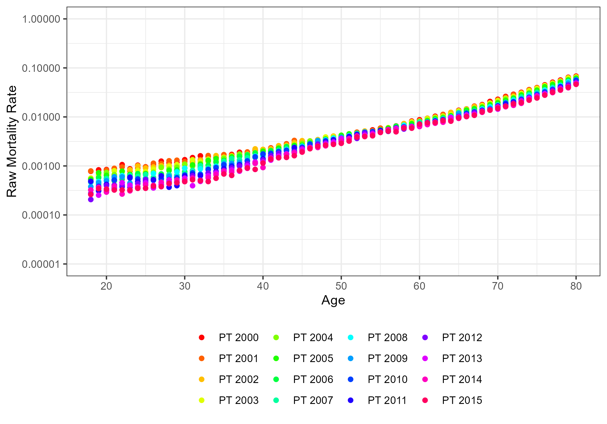
The usage of the \codeblc function to fit the Bayesian Lee-Carter model results in an object of class \code"BLC". In this example, we consider the default settings to fit the BLC model with the code: {CodeChunk} {CodeInput} R> fit.blc <- blc(Y, numit = 2000) Simulating [===================================] 100 The \codefitted function returns the fitted log mortality estimates for each year. For the \code"BLC" object, the function returns an object of type \codelist containing log mortality means (\code$mean) as well as credible intervals (\code$lower and \code$upper). The \codeplot function is called to visualize the evolution of the fitted log mortality estimates through the years (Figure 18). The output from the function \codefitted for ages 18-23 and years 2000-2003 and call to the \codeplot function are shown as follows: {CodeChunk} {CodeInput} R> head(fitted(fit.blc)[[1]][,1:4]) 2000 2001 2002 2003 18 0.0007230827 0.0006849759 0.0006474087 0.0006217643 19 0.0007610521 0.0007242883 0.0006878730 0.0006629022 20 0.0008571602 0.0008135041 0.0007703697 0.0007408658 21 0.0008284950 0.0007906396 0.0007529585 0.0007271215 22 0.0009426982 0.0008926108 0.0008432942 0.0008096202 23 0.0008562065 0.0008166684 0.0007775165 0.0007504693 R> plot(fit.blc, parameter = "fitted", ages = 18:80)

The evolution of the mortality graduation can be seen through the , and parameters. Figure 19 depicts the fitted parameters of the BLC model using the \codeplot method for the \code"BLC" class. {CodeChunk} {CodeInput} R> plot(fit.blc, parameter = "all", ages = 18:80)

From Figure 19 we see that the parameter displays the general mortality pattern present in the data. Notice that the parameter which represents the global level of mortality in period is decreasing through the years. This behaviour impacts the interpretation of parameter directly. In this case, is also called improvement and reflects the rate at which mortality is decreasing over the years. In the package \pkgBayesMortalityPlus the improvement of the BLC model is implemented via the function \codeimprovement. This function estimates the improvement percentage for each age throughout the whole considered time interval. {CodeChunk} {CodeInput} R> head(improvement(fit.blc, cred = 0.95)) improvement lower.lim upper.lim 1 0.06566689 0.04441260 0.08594036 2 0.06024696 0.04458217 0.07688504 3 0.06355622 0.05544481 0.07100160 4 0.05708944 0.04320909 0.07150397 5 0.06620879 0.05008862 0.08211478 6 0.05758188 0.04366629 0.07128359 The \codeexpectancy and \codeHeatmap methods are available to compute life expectations and their uncertainty via credible intervals for each age and year. For instance, we consider specific ages using the argument \code“at” and the output can be obtained with the commands: {CodeChunk} {CodeInput} R> expectancy(fit.blc, at = c(1,21,41,61))expectancy[,1:4] 2000 2001 2002 2003 18 55.844 55.997 56.153 56.262 38 36.942 37.042 37.145 37.218 58 18.983 19.053 19.124 19.175 78 2.646 2.655 2.663 2.669 The plot of life expectancy (see Figure 20) can be produced using the code: {CodeChunk} {CodeInput} R> Heatmap(fit.blc, x_lab = 2000:2015, age = 18:80) + scale_x_discrete(breaks = seq(2000,2015, by=3))

Forecast for fitted BLC models
In the package \pkgBayesMortalityPlus the forecasting of the BLC mortality model for n-years ahead is implemented via the \codepredict function. Following Pedroza 2006 the predictive steps can be incorporated into the Gibbs sampler. The posterior predictive distribution for future observations can be expressed as
where represents the model parameters. We assume that and are conditionally independent given .
The prediction can be obtained by the basic \codepredict function, specifying the years ahead to be forecasted by the \codeh argument, resulting in an object of class \code"PredBLC". The output considers 10-years-ahead () for the Portugal mortality experience: {CodeChunk} {CodeInput} R> fit.blc2 <- predict(fit.blc, h = 10) R> print(fit.blc2) Forecast of a Bayesian Lee-Carter model (h = 10)
The functions such as \codefitted, \codeexpectancy and \codeHeatmap also are available for the \code"PredBLC" object. See below: {CodeChunk} {CodeInput} R> head(fitted(fit.blc2)expectancy[,1:4] [,1] [,2] [,3] [,4] [1,] 58.274 58.389 58.501 58.615 [2,] 38.679 38.770 38.858 38.950 [3,] 20.200 20.265 20.327 20.392 [4,] 2.779 2.786 2.792 2.798
R> Heatmap(fit.blc2, x_lab = 2016:2025, age = 18:80) + scale_x_discrete(breaks = seq(2016,2025, by=3))

6 Conclusions
In this paper, we present an \proglangR package called \pkgBayesMortalityPlus for mortality modelling using a Bayesian approach. The package allows for Bayesian inference for several models used for mortality table graduation as well as mortality prediction for future years. The tools available in the proposed package provide model fitting, visualization of parameters and linear and non-linear functions of parameters, and uncertainty quantification via credible intervals or complete posterior distributions. Examples are provided to illustrate the features of all models. For the Heligman-Pollard law of mortality, Bayesian model fitting is available for three probability distributions: Poisson, Binomial and Log-Normal. The interpretable parameters in the HP model can be visualised through graphs and summaries of the resulting posterior distributions. As an alternative to spline fitting for mortality graduation, the \codedlm function takes into account the autocorrelation in the mortality across ages and provides estimation of mortality curves and extrapolation for older ages. Opposed to the HP model, DLM fit does not depend on a specific law of mortality for the data. Smoothness is controlled by discount factors, which are common practice in the context of time series modelling via dynamic models, and offer flexibility to the model of death probabilities. Lastly, the Bayesian version of the well-known Lee-Carter model is implemented via MCMC methods and the \codepredict function allows for prediction in future time steps. Furthermore, point estimates, as well as uncertainty measurements, can be computed for improvement parameters which are often the main interest in studies of longevity and pricing of products of long term in insurance modelling.
Acknowledgments
We are grateful to LabMA/UFRJ (Laboratório de Matemática Aplicada of the Universidade Federal do Rio de Janeiro) based in Brazil for financial support and to its members for the very enriching discussions.
References
- Banerjee et al. (2004) Banerjee S, Carlin BP, Gelfand AE (2004). Hierarchical Modeling and Analysis for Spatial Data. Monographs on Statistics and Applied Probability 101, 1 edition. Chapman & Hall/CRC.
- Barigou and Goffard (2022) Barigou K, Goffard PO (2022). StanMoMo: Bayesian Mortality Modelling with ’Stan’. R package version 1.1.0, URL https://CRAN.R-project.org/package=StanMoMo.
- Booth et al. (2002) Booth H, Maindonald JH, Smith L (2002). “Applying Lee-Carter under conditions of variable mortality decline.” Population Studies, 56, 325 – 336.
- Bowers (1986) Bowers N (1986). Actuarial Mathematics. 1 edition. Society of Actuaries. ISBN 9780938959106. URL https://books.google.com.br/books?id=jrjuAAAAMAAJ.
- Camarda (2012) Camarda CG (2012). “MortalitySmooth: An R Package for Smoothing Poisson Counts with P-Splines.” Journal of Statistical Software, 50(1), 1–24. URL http://www.jstatsoft.org/v50/i01/.
- Camarda (2019) Camarda CG (2019). “Smooth constrained mortality forecasting.” Demographic Research, 41(38), 1091–1130. 10.4054/DemRes.2019.41.38. URL https://ideas.repec.org/a/dem/demres/v41y2019i38.html.
- Camarda et al. (2016) Camarda CG, Eilers PH, Gampe J (2016). “Sums of smooth exponentials to decompose complex series of counts.” Statistical Modelling, 16(4), 279–296. 10.1177/1471082X16641796. URL https://doi.org/10.1177/1471082X16641796.
- Carlin (1992) Carlin BP (1992). “A simple Monte Carlo approach to Bayesian graduation.” In Transactions of the Society of Actuaries. Citeseer.
- Carter and Kohn (1994) Carter C, Kohn R (1994). “On Gibbs sampling for state space models.” Biometrika, 81(3), 541–553.
- Currie et al. (2004) Currie ID, Durban M, Eilers PH (2004). “Smoothing and forecasting mortality rates.” Statistical Modelling, 4(4), 279–298. 10.1191/1471082X04st080oa. URL https://doi.org/10.1191/1471082X04st080oa.
- Czado et al. (2005) Czado C, Delwarde A, Denuit M (2005). “Bayesian Poisson log-bilinear mortality projections.” Insurance: Mathematics and Economics, 36(3), 260–284. ISSN 0167-6687. https://doi.org/10.1016/j.insmatheco.2005.01.001. URL https://www.sciencedirect.com/science/article/pii/S0167668705000302.
- Dellaportas et al. (2001) Dellaportas P, Smith AF, Stavropoulos P (2001). “Bayesian analysis of mortality data.” Journal of the Royal Statistical Society: Series A (Statistics in Society), 164(2), 275–291.
- Dodd et al. (2018) Dodd E, Forster J, Bijak J, Smith P (2018). “Smoothing mortality data: the English life table, 2010-12.” Journal of the Royal Statistical Society: Series A (Statistics in Society), 181(3), 717–735.
- Frühwirth-Schnatter (1994) Frühwirth-Schnatter S (1994). “DATA AUGMENTATION AND DYNAMIC LINEAR MODELS.” Journal of Time Series Analysis, 15(2), 183–202. 10.1111/j.1467-9892.1994.tb00184.x.
- Gamerman and Lopes (2006) Gamerman D, Lopes H (2006). Markov Chain Monte Carlo: Stochastic Simulation for Bayesian Inference. Texts in Statistical Science, 2 edition. Taylor & Francis.
- Gavrilov and Gavrilova (2011) Gavrilov LA, Gavrilova NS (2011). “Mortality measurement at advanced ages: a study of the Social Security Administration Death Master File.” North American actuarial journal, 15(3), 432–447.
- Gompertz (1825) Gompertz B (1825). “XXIV. On the nature of the function expressive of the law of human mortality, and on a new mode of determining the value of life contingencies. In a letter to Francis Baily, Esq. FRS &c.” Philosophical transactions of the Royal Society of London, 115, 513–583.
- Heligman and Pollard (1980) Heligman L, Pollard JH (1980). “The age pattern of mortality.” Journal of the Institute of Actuaries, 107(1), 49–80.
- Hilton et al. (2019) Hilton J, Dodd E, Forster JJ, Smith PW (2019). “Projecting UK mortality by using Bayesian generalized additive models.” Journal of the Royal Statistical Society, Series C (Applied Statistics), 68(1), 29–49.
- HMD (2022) HMD (2022). “Human Mortality Database. Max Planck Institute for Demographic Research (Germany), University of California, Berkeley (USA), and French Institute for Demographic Studies (France).” https://www.mortality.org/. Accessed: 2022-07-28.
- Hustead (2005) Hustead EC (2005). “Ending the mortality table.” In Living to 100 and Beyond Symposium.
- Hyndman and Shahid Ullah (2007) Hyndman RJ, Shahid Ullah M (2007). “Robust forecasting of mortality and fertility rates: A functional data approach.” Computational Statistics & Data Analysis, 51(10), 4942–4956. ISSN 0167-9473. https://doi.org/10.1016/j.csda.2006.07.028.
- Kimeldorf and Jones (1967) Kimeldorf G, Jones DA (1967). “Bayesian graduation.” Transactions of the Society of Actuaries, 19(54 part 1), 66–112.
- Lai (2012) Lai C (2012). “Human mortality curves that decelerate to a plateau.” Mathematical and Computer Modelling, 55(3-4), 1118–1128.
- Lee and Carter (1992) Lee R, Carter L (1992). “Modeling and forecasting U.S. mortality.” Journal of the American Statistical Association, 87(419), 659–671. 10.2307/2290201.
- Lee and Miller (2001) Lee R, Miller T (2001). “Evaluating the performance of the Lee-Carter method for forecasting mortality.” Demography, 38, 537–549. 10.2307/3088317.
- Li (2013) Li J (2013). “A Poisson common factor model for projecting mortality and life expectancy jointly for females and males.” Population Studies, 67(1), 111–126. 10.1080/00324728.2012.689.
- Li et al. (2004) Li N, Lee RD, Tuljapurkar S (2004). “Using the Lee–Carter method to forecast mortality for populations with limited data.” International Statistical Review, 72, 19–36.
- Neves and Migon (2007) Neves C, Migon HS (2007). “Bayesian graduation of mortality rates: An application to reserve evaluation.” Insurance: Mathematics and Economics, 40, 424–434.
- Pascariu (2022) Pascariu MD (2022). MortalityLaws: Parametric Mortality Models, Life Tables and HMD. R package version 1.9.3, URL https://CRAN.R-project.org/package=MortalityLaws.
- Pedroza (2006) Pedroza C (2006). “A Bayesian forecasting model: predicting U.S. male mortality.” Biostatistics, 7(4), 530–550. ISSN 1465-4644. 10.1093/biostatistics/kxj024. https://academic.oup.com/biostatistics/article-pdf/7/4/530/610324/kxj024.pdf, URL https://doi.org/10.1093/biostatistics/kxj024.
- Petris et al. (2009) Petris G, Petrone S, Campagnoli P (2009). “Dynamic linear models.” In Dynamic linear models with R, pp. 31–84. Springer.
- R Core Team (2020) R Core Team (2020). R: A Language and Environment for Statistical Computing. R Foundation for Statistical Computing, Vienna, Austria. URL https://www.R-project.org/.
- Renshaw et al. (1996) Renshaw A, Haberman S, Hatzopoulos P (1996). “The Modeling of Recent Mortality Trends in United Kingdom Male Assured Lives.” British Actuarial Journal, 2. 10.1017/S1357321700003470.
- Rob J Hyndman et al. (2019) Rob J Hyndman wcfHB, Tickle L, Maindonald J (2019). demography: Forecasting Mortality, Fertility, Migration and Population Data. R package version 1.22, URL https://CRAN.R-project.org/package=demography.
- Sharrow (2012) Sharrow DJ (2012). HPbayes: Heligman Pollard mortality model parameter estimation using Bayesian Melding with Incremental Mixture Importance Sampling. R package version 0.1, URL https://CRAN.R-project.org/package=HPbayes.
- Sherris and Njenga (2011) Sherris M, Njenga C (2011). “Modeling mortality with a Bayesian vector autoregression.” Technical report, Research Paper 2011ACTL04. Australian School of Business, University of New South Wales, Sydney.
- Stan Development Team (2020) Stan Development Team (2020). “RStan: the R interface to Stan.” URL http://mc-stan.org/.
- Tang et al. (2021) Tang K, Dodd E, Forster J (2021). “Joint modelling of male and female mortality rates using adaptive P-splines.” Annals of Actuarial Science, 16, 1–17. 10.1017/S1748499521000105.
- Turner and Firth (2022) Turner H, Firth D (2022). Generalized nonlinear models in R: An overview of the gnm package. R package version 1.1-2, URL https://cran.r-project.org/package=gnm.
- Villegas et al. (2018) Villegas AM, Kaishev VK, Millossovich P (2018). “StMoMo: An R Package for Stochastic Mortality Modeling.” Journal of Statistical Software, 84(3), 1–38. 10.18637/jss.v084.i03.
- West and Harrison (1997) West M, Harrison J (1997). Bayesian forecasting and dynamic models. 2 edition. Springer.
- Wickham et al. (2022) Wickham H, François R, Henry L, Müller K (2022). dplyr: A Grammar of Data Manipulation. R package version 1.0.9, URL https://CRAN.R-project.org/package=dplyr.
- Wood (2006) Wood SN (2006). Generalised Additive Models: an Introduction with R. 1 edition. Boca Raton: Chapman and Hall– CRC.