Efficient Reinforcement Learning with Impaired Observability: Learning to Act with Delayed and Missing State ObservationsThanks: Correspondence to Mengdi Wang. Emails: minshuochen, mengdiw@princeton.edu
Abstract
In real-world reinforcement learning (RL) systems, various forms of impaired observability can complicate matters. These situations arise when an agent is unable to observe the most recent state of the system due to latency or lossy channels, yet the agent must still make real-time decisions. This paper introduces a theoretical investigation into efficient RL in control systems where agents must act with delayed and missing state observations. We present algorithms and establish near-optimal regret upper and lower bounds, of the form , for RL in the delayed and missing observation settings. Here and are the sizes of state and action spaces, is the time horizon and is the number of episodes. Despite impaired observability posing significant challenges to the policy class and planning, our results demonstrate that learning remains efficient, with the regret bound optimally depending on the state-action size of the original system. Additionally, we provide a characterization of the performance of the optimal policy under impaired observability, comparing it to the optimal value obtained with full observability. Numerical results are provided to support our theory.
1 Introduction
In Reinforcement Learning (RL), an agent engages with an environment in a sequential manner. In an ideal setting, at each time step, the agent would observe the current state of the environment, select an action to perform, and receive a reward (Smallwood and Sondik 1973; Bertsekas 2012; Sutton and Barto 2018; Lattimore and Szepesvári 2020). However, real-world engineering systems often introduce impaired observability and latency, where the agent may not have immediate access to the instantaneous state and reward information. In systems with lossy communication channels, certain state observations may even be permanently missing, never reaching the agent. Nonetheless, the agent still needs to make real-time decisions based on the available information.
The presence of impaired observability transforms the system into a complex interactive decision process (Figure 1), presenting challenges for both learning and planning in RL. With limited knowledge about recent states and rewards, the agent’s policy must extract information from the observed history and utilize it to make immediate decisions. This introduces significant complexity to the policy class and poses difficulties for RL. Moreover, the loss of information due to permanently missing observations further hampers the efficiency of RL methods. Although a naïve approach would involve augmenting the state and action space to create a fully observable Markov Decision Process (MDP), such a method would lead to exponential regret growth in the state-action size.
Why existing methods do not work
One may be tempted to cast the problem of impaired observability as a Partially Observed MDP (POMDP) problem. However, this would not solve the problem. In a POMDP, the system does not reveal its instantaneous state to the agent but provides an emission state observation conditioned on the latent state. POMDPs are known to suffer from the curse of history (Papadimitriou and Tsitsiklis 1987; Bertsekas 2012; Krishnamurthy 2016), unless additional assumptions are imposed. Existing efficient algorithms focus on subclasses of POMDPs with decodable or distinguishable partial observations (Jin et al. 2020; Uehara et al. 2022; Zhan et al. 2022; Chen et al. 2022; Liu et al. 2022; Zhong et al. 2022; Chen et al. 2023), where the unseen instantaneous state can be inferred from recent observations. Unfortunately, MDPs with impaired observability do not fall into these benign subclasses. The reason behind this is that at each time step, a new observation, if any, is in fact a past state. Viewing it as an emission state of the current one leads to a time reversal posterior distribution depending on the underlying transitions, which suffers from the curse of history and makes the POMDP intractable. The problem becomes even worse if some observations are missing.
Empirical evidence suggests that efficient RL is possible even with impaired state observability (Lizotte et al. 2008; Liu et al. 2014; Agarwal and Aggarwal 2021). However, theoretical understanding of this problem is very limited. One notable work Walsh et al. 2007 studied learning with constant-time delayed observations. It identified subclasses of MDPs with nearly deterministic transitions that can be efficiently learned. Beyond this special case, efficient RL with impaired observability in MDPs with fully generality remains largely open.
Some recent works have studied delayed feedback in MDPs (Yang et al. 2023; Howson et al. 2023). This is a different problem where the agent’s policy can still access real-time states but learning uses delayed data. Our problem is fundamentally harder because the agent’s policy can only access the lossy and delayed history. See Section 1.1 for more discussions.
Our results
In this paper, we provide algorithms and regret analyses for learning the optimal policy in tabular MDPs with impaired observability. Note that this optimal policy is a different one from the optimal policy with full observability. To approach this problem, we construct an augmented MDP formulation where the original state space is expanded to include available observations of past states and an action sequence. However, the expanded state space is much larger than the original one and naïve application of known methods would lead to exponentially large regret bounds. In our analyses, we exploit the structure of the augmented transition model to achieve efficient learning and sharp regret bounds. The main results are summarized as follows.
For MDPs with stochastic delays, we prove a regret bound (Theorem 4.1) compared to the best feasible policy. Here and are the sizes of the original state and action spaces, respectively, is the horizon, is the maximal length of delay, and is the number of episodes. We allow the delay to be stochastic and conditionally independent given the current state and action. Accompanying the regret upper bound, we derive a lower bound in Proposition 4.3. Moreover, we quantify the performance degradation of the optimal value due to impaired observability, compared to the optimal value for fully observable MDPs (Proposition 4.5). We also showcase in Proposition 4.6 that a short delay does not reduce the optimal value, but slightly longer delay leads to substantial degradation.
For MDPs with randomly missing observations, we provide an optimistic RL method that provably achieves regret (Proposition 5.1). We also provide a sharper regret in the case when the missing rate is sufficiently small (Theorem 5.2).
To our best knowledge, these results present a first set of theories for RL with delayed and missing observations. Remarkably, our regret bounds nearly match the minimax-optimal regret of standard MDP in their dependence on and (noting that the target optimal policies are different in the two cases). These results imply that RL with impaired observability is provably as efficient as RL with full observability (up to poly factors of ).

1.1 Related Work
Efficient algorithms for learning in the standard setting of tabular MDPs without impaired observability have been extensively studied (Kearns and Singh 2002; Brafman and Tennenholtz 2002; Jaksch et al. 2010; Dann and Brunskill 2015; Azar et al. 2017; Agrawal and Jia 2017; Jin et al. 2018; Dann et al. 2019; Zanette and Brunskill 2019; Zhang et al. 2020; Domingues et al. 2021), where the minimax optimal regret is (Azar et al. 2017; Domingues et al. 2021).
The delayed observation model studied in this paper is related to delayed feedback model in Howson et al. 2023; Yang et al. 2023, yet the setup is fundamentally different. In delayed feedback, an agent sends a policy to the environment for execution. The environment executes the policy on behalf of the agent for an episode, but the whole trajectory will be returned to the agent after some episodes. The policy executed by the environment is able to “see” instantaneous states and rewards. It is Markovian and is not played by the agent. Our setting concerns learning executable policies when delayed or missing states appear within an episode. The policy is no longer Markovian and can only prescribe action based on history. Therefore, the algorithms and analyses for delayed feedback MDPs are not applicable to our settings.
Despite the distinct settings, there are existing fruitful results in efficiently learning MDPs or bandits with delayed feedback. Stochastic delayed feedback in bandits is studied in Agarwal and Duchi 2011; Dudik et al. 2011; Joulani et al. 2013; Vernade et al. 2017; Vernade et al. 2020; Gael et al. 2020; Lancewicki et al. 2021. In a more challenging setting of reinforcement learning, Howson et al. 2023 considers tabular MDPs and Yang et al. 2023 generalizes to MDPs with function approximation and multi-agent settings.
On the other hand, results analyzing MDPs with missing observations are limited in the literature, although missing data is a commonly recognized issue in applications (García-Laencina et al. 2010; Jerez et al. 2010; Little et al. 2012; Emmanuel et al. 2021). One notable result is presented in Bouneffouf et al. 2020 for bandits with missing rewards.
1.2 MDP Preliminaries
An episodic MDP is described by a tuple , where are state and action spaces, respectively, is the horizon, is the reward function and is the transition probability. We primarily focus on tabular MDPs, where and are both finite. We also assume that the reward is uniformly bounded with for any . An agent will interact with the environment for episodes, hoping to find a good policy to maximize the cumulative reward. Within an episode, at the -th step, the agent chooses an action based on the available information about the environment. After taking the action, the underlying environment produces a reward and transits to the next state. With full state observation, a policy maps the instantaneous state to an action or an action distribution. Given such a policy , the value function is where is the policy induced expectation.
Notation: For real numbers , and as the smallest integer larger than . In episodic MDPs, we use a superscript to denote the index of episodes, and a subscript to denote the index of time. We denote as the collection of actions from time to . For two probability distributions and , we denote their total variation distance as .
2 Problem formulation
In this work, we study MDPs with impaired observability. We focus on two practical settings: 1) delayed observations and 2) missing observations.
2.1 MDPs with Delayed Observations
In any episode, we denote as the observational delay of the state and reward at step . That is, we receive and at time . The delay time can be dependent on the state and action at time . To facilitate analysis, we denote the inter-arrival time between the arrival of observations for step and as . With delays, at time , the nearest observable state is denoted as , where . Then the executable policy class
chooses actions depending on the nearest visible state and history actions. We impose the following assumption on the interarrival times.
Assumption 2.1 .
The interarrival time takes value in . The distribution of can depend on , but is conditionally independent of the MDP transitions given . Furthermore, we denote the maximum length of delay as .
Assumption 2.1 does not impose any specific distributional assumption on , but only requires that the delayed observations arrive in order and that, at each time step, there is at most one new visible state and reward pair (). A widely studied example of delays in the literature is that the inter-arrival time is geometrically distributed (Winsten 1959). Then the observation sequence is a Bernoulli process, which can be thought of as a discretized version of a Poisson process.
Our delayed observation setting is newly proposed and substantially generalizes the Constant Delayed MDPs (CDMDPs) studied in Brooks and Leondes 1972; Bander and White III 1999; Katsikopoulos and Engelbrecht 2003; Walsh et al. 2007. When being deterministic for all and , our observation delay coincides with CDMDPs. In CDMDPs, a new past observation is guaranteed to arrive at each time step. However, in contrast, our delay model can result in no new observation at some time steps.
Observation delay leads to difficulty in planning, as the agent can only infer the current state and then choose an action. Therefore, the policy is naturally history dependent. We summarize the interaction protocol of the agent with the environment in Protocol 1.
At the end of each episode, we can collect all delayed observations, however, these observations are not used in planning. In reality, the agent can collect these observations by waiting after time . Protocol 1 is similar to hindsight observability in POMDPs studied in Lee et al. 2023. Yet their analysis for POMDPs is not directly transferable to our settings as mentioned in the introduction.
2.2 MDPs with Missing Observations
In addition to the stochastic delay in observations, we also consider randomly missing observations. In applications, an agent interacts with the environment through some communication channel. The communication channel is often imperfect and thus, observation can be lost during transmission. This type of missing observation is permanent and we describe in the following assumption.
Assumption 2.2 .
Any observation pair (state and reward) is independently observable in the communication channel. The observation rate is depending on , but independent of the MDP transitions. Moreover, there exists a constant such that for all . The agent will be informed when an observation is missing.
3 Construction of Augmented MDPs
To tackle the limited observability, we expand the original state space and define an augmented MDP. It will serve as the basis for our subsequent theoretical analysis.
3.1 Augmented MDP with Expected Reward
In the remainder of this section, we focus on the delayed observation case and defer the missing observation case to Section 5. Define as an augmented state, where is the number of steps without receiving new observations after observing . Let denote the augmented state space of all possible ’s. Then the original MDP with delayed observations can be reformulated into a state-augmented one . The reward is defined as
which is the expected reward given the nearest past state and historical actions . We can define a belief distribution so that . Belief distributions are widely adopted in partially observed MDPs (Ross et al. 2007; Poupart and Vlassis 2008). Yet the belief propagation with delayed observations is not Markovian and is rather complicated compared to that in POMDPs. We will frequently use the belief distribution to study the expressivity of in Section 4.3.
The transition probabilities are sparse. For any and , we have
where indicates whether or not the rolling actions are matched, i.e.,
and is defined as
The factored form of follows from the conditional independence in Assumption 2.1. We define -functions and value functions as follows. For any and policy , we have
We note that is equivalent to for the same executable policy . We also denote as the transition operator corresponding to . It can be checked that
also makes all the policies in executable and Markovian. Meanwhile, the reward function keeps track of the expected reward for all . Although the expanded state space is much more complicated than the original state space , the sparseness of the transition probabilities still allow for efficient exploration. We note that depends only on the delay distribution and one-step Markov transitions. However, there is still one caveat for learning in – the reward function depends on the belief distributions, which involve multi-step transitions.
3.2 Augmented MDP with Past Reward
To tackle the aforementioned challenge, we further define which shares the optimal policy in with an enlonged horizon . The state space consists of any . Comparing to , we cut off the action at horizon , since for has no influence on the state and reward during . The reward function is defined as
By definition, is a past reward. More importantly, zeros out rewards outside the original horizon . Meanwhile, between the arrival of two consecutive state observations, the reward only counts once. Lastly, the transition probabilities are
We interpret the transitions as follows. When , the transition is the same as . When , we simply wait for unobserved states and rewards to come. As mentioned, actions taken beyond time are irrelevant. The following proposition asserts an equivalence between the value functions in and .
Proposition 3.1.
Let and be defined as in the previous paragraphs. Then for any initial state and any policy , it holds that
where in the right-hand side, the policy for steps to is arbitrary.
4 RL with Delayed Observations and Regret Analysis
In this section, we provide a regret analysis of learning in MDPs with stochastic delays. For the sake of simplicity, we assume the reward is known, however, extension to unknown reward causes no real difficulty. Motivated by the augmented MDP reformulation, we introduce our learning algorithm in Algorithm 2. In Line 5, unobserved states and rewards are returned to the agent as described in Protocol 1. Using the data set, we construct bonus functions compensating for the uncertainty in one-step transitions of the original MDP. This largely sharpens the confidence region, yet still ensures a valid optimism. We emphasize that in Line 9, we are planning on involving the augmented transitions and expanded states of . Only in this way, can we obtain an executable policy in delayed MDPs.
4.1 Regret Bound
We define the regret in delayed MDP as
where is the value function of the original MDP. Although the regret here is defined on the original MDP, it is equivalent to the regret of the same policy on and further by Proposition 3.1. Note that we are comparing with the best executable policy. The performance degradation caused by observation delay is discussed in Section 4.3. The following theorem bounds the regret.
Theorem 4.1 (Regret Bound for Delayed MDPs).
The proof is provided in Appendix B.1. We now discuss several implications.
Sharp dependence on and
Theorem 4.1 has a sharp dependence on and , although the expanded state space has a cardinality bounded by . Naïvely learning and planning in would suffer from the exponential enlargement of . However, we identify the sparse structures in the transition probabilities. As can be seen, involves only one-step transitions in the original MDP and some conditionally independent delay distributions. Such structures lead to a rather easy estimation of , which can be constructed from the estimators of one-step transitions in the original MDP. Meanwhile, the sparse structures make exploration in efficient.
Influence of the delay distribution
Theorem 4.1 holds for arbitrary conditionally independent delay distributions, even including heavy-tailed distributions. In the worst case of unbounded delays, Theorem 4.1 gives rise to a regret. The reason for this is that if the delay is larger than , then the corresponding state will only be observed after an episode ends and will not be used in planning. Therefore, we can truncate the delay at , regardless of its tail distributions.
When the maximal length of delay , e.g., CDMDPs with for any , Theorem 4.1 implies that the regret is bounded by
We observe that as the length of delay increases, the regret bound enlarges, reflecting the increased difficulty of long delays. Moreover, when corresponding to no delays, we recover the standard regret bound in tabular MDPs (Azar et al. 2017, Theorem 1). We remark that Theorem 4.1 can be directly extended to being a high probability upper bound on the length of delay. Yet, the analysis causes no real difficulty and is omitted.
Extension to discounted MDPs
Our algorithm and regret analysis are applicable to episodic infinite-horizon discounted MDPs. Since the reward is uniformly bounded by , we can truncate the horizon so that the tail accumulative reward contributes negligibly. In this way, we convert the infinite-horizon MDP to a finite-horizon MDP. Then we have the following corollary.
Corollary 4.2.
4.2 Lower Bounds on Regret and Planning Complexity
We first show an accompanying lower bound on the regret and demonstrate the influence of the length of delay.
Proposition 4.3.
Let be an integer and consider CDMDPs with length of delay . Suppose , , , and . Then for any learning algorithm, there exists a hard MDP instance such that
where the expectation is taken over the randomness in the algorithm and the MDP instance.
The proof is provided in Appendix B.5. The lower bound in Proposition 4.3 indicates increased complexity when the length of delay increases. Meanwhile, the dependence on and matches that in the upper bound (Theorem 4.1). It is noted that there is still a gap between the upper and lower bound in terms of the dependence on and . We suspect that the lower bound can be further improved; nonetheless, detailed investigation of this issue is left as a future research direction.
We next shift our attention to the planning complexity with delayed observations. It is noted that in the worst case, the planning complexity in Algorithm 2 grows exponentially with respect to the length of delay. Unfortunately, this is inevitable even for CDMDPs.
Proposition 4.4 (Theorem 2 in Walsh et al. 2007).
The general CDMDP planning problem is NP-Hard.
Yet, there are special subclasses of MDPs still allow a polynomial-time planning, such as nearly deterministic MDPs identified in Walsh et al. 2007. While investigating polynomial planning algorithms for specific problem is beyond the scope of this paper, we believe that our augmented MDP formation is compatible with practical planning oracle for accelerated solution of RL.
4.3 Performance Degradation Caused by Delays
This section is devoted to quantifying the performance degradation caused by delayed observations. In particular, we bound the value difference between the best executable policy and the best Markov policy in a no delay environment. Recall that is the value function of the original MDP. We denote
as the best vanilla optimal policy and executable policy, respectively. The values achieved by and are denoted as and , respectively. The gap between and quantifies the performance degradation, which is denoted as
We bound gap in Proposition 4.5.
Proposition 4.5.
In the setup of Section 4.3, we have
where and are visitation measures induced by and , respectively.
The proof is provided in Appendix B.3. The term is nonnegative due to the convexity of the max operator. The term accounts for the difference in the visitation measure. When the original MDP has deterministic transitions, we can check that is zero, since the expectation over is concentrated on a singleton that can be inferred from history. Hence, the visitation measures are also identical, which implies . On the contrary, when is evenly spread, meaning that the entropy of is high, we potentially suffer from a large performance drop, in that inferring the current state is difficult.
4.4 (Mysterious) Effect of Delay on the Optimal Value
To further understand the effect of the delay on the optimal value, we provide the following dichotomy. On the one hand, we show that there exists an MDP instance, such that a constant delay of steps does not hurt the performance. On the other hand, in the same MDP instance, a constant delay of steps results in a constant performance drop.
Proposition 4.6.
Consider constant-delayed MDPs. Fix a positive integer . Then there exists an MDP instance such that the following two items hold simultaneously.
When the delay is , it holds that .
When the delay is , it holds that , with probability .
The proof is provided in Appendix B.4. We remark that Proposition 4.6 says that observation delay can be dangerous, even with the slightest possible number of steps. The idea behind Proposition 4.6 is consistent with the analysis on gap. In particular, we construct an MDP instance demonstrated in Figure 2, where the reward vanishes at all times but . When the delay is , the initial state is revealed and the policy can choose the best action to receive a reward. When the delay is , however, there is always a probability of missing the best action for any policy, which leads to a constant performance degradation.
5 RL with Missing Observations and Regret Analysis
We now switch our study to MDPs with missing observations. In such an environment, executable policies share the same structures as delayed MDPs, where an action is taken based on available history information. Compared to delayed observations, learning with missing observations is more challenging. Since unobserved states and rewards are never recovered, we suffer from information loss. Moreover, we will frequently deal with multi-step transitions, due to missing observations between two consecutive visible states.
5.1 Optimistic Planning with Missing Observations
Despite the difficulty, we present here algorithms that are efficient in learning and planning for MDPs with missing observations. We begin with an optimistic planning algorithm in Algorithm 3. To unify the notation, we denote and to indicate missing the corresponding observation.
Most of this algorithm resembles the typical optimistic planning (Jaksch et al. 2010) but with some notable differences. In Line 4, the value function is for the original MDP with transition probabilities parametrized by . Different from the typical optimistic planning, the underlying MDP here obeys the stochastic observable model in Assumption 2.2. Therefore, the value is the sum of all possible values under missing observations. When counting in Line 6, we exclude data tuples missing the next state, which inevitably slows down the learning curve. Nonetheless, the effect of missing only contributes as a scaling factor in the regret.
Proposition 5.1.
The proof is provided in Appendix C.1. Proposition 5.1 is optimal in the dependence and achieves an dependence on the complexity of the underlying MDP. In the extreme case of , which implies that every state and reward are hardly observable, we have . Here is the probability of observing two consecutive states for estimating the transition probabilities. Proposition 5.1 requires the knowledge of observable rate . This is not a restrictive condition, as estimating from Bernoulli random variables is much easier than estimating transition probabilities.
5.2 Model-Based Planning using Augmented MDPs
Proposition 5.1 is not sharp in the dependence on . We next show that the augmented MDP approach is effective to tackle missing observations, when the observable rate satisfies additional conditions. Specifically, we assume that the observable rate is independent of . We utilize the reformulation, except that we redefine the transition probabilities as
The first case in corresponds to receiving the state observation at time . In contrast to the delayed MDPs, the transition probabilities here potentially rely on multi-step transitions in the original MDP. The second case of the transition corresponds to missing the observation. We summarize the policy learning procedure in Algorithm 4.
We remark that similar to delayed MDPs, in Line 9 the planning is on and the obtained policy is executable given any when state observation is missed. Therefore, the planning complexity is . Different from Algorithm 2, the bonus function here depends on multi-step transitions, in that missing observations are permanently lost. The following theorem shows that Algorithm 4 is asymptotically efficient when the observable rate is relatively high.
Theorem 5.2.
The proof is provided in Appendix C.2. Some remarks are in order.
rate when is large
When the number of episodes , the first term in the regret bound dominates and attains a sharp dependence on and . However, when the number of episodes are limited, the regret bound has a worse dependence on the state space size . We also observe that as the missing rate becomes small (equivalently, becomes large), the regret is close to .
Observable rate smaller than
Theorem 5.2 holds for an observable rate . The intuition behind this is that, to fully explore all the actions when a state observation is missing takes trials. Therefore, in expectation, we will encounter a missing observation at least every episodes as long as . Nonetheless, when , the regret bound remains curiously underexplored. We conjecture that is a critical point distinguishing unique strategies for learning and planning in MDPs with missing observations. A detailed analysis of this issue goes beyond the scope of the current paper.
Proof sketch
The proof of Theorem 5.2 adapts the analysis of model-based UCBVI algorithms Azar et al. 2017. Let denote the maximal length of consecutive missing observations. We denote as the event when the maximal length of consecutive missing is less than . On event , a naïve analysis leads to a regret, in observation to the size of the expanded state space . However, our analysis circumvents the dependence by exploiting the occurrence of consecutive missing observations is rare (Lemma C.3). On the complement of event , the regret is bounded by . Summing up the two parts and choosing a proper yield our result.
6 Numerical Experiment with Delayed Observations
This section presents synthetic data experiments to validate our theory on MDPs with delayed observations.
Tabular MDP instance
We focus on a 20-state 5-action MDP instance, i.e., and . The horizon is set to be and we vary the maximal length of delay in . We use to index the state and to index the action. The reward function is set as
which implies that the optimal policy should maximally maintain a large visitation measure on state and to receive a nonzero reward.
We specify two sets of transition probabilities being time-homogeneous, corresponding to nearly deterministic and more stochastic transitions, respectively. Specifically, for nearly deterministic transitions (Env1), we set as a special action that moves states towards the nonzero reward state and . The transition probabilities are
| (6.1) |
As opposed to the special action , all the other actions leads the state to either or , which will not receive a reward. The transition probabilities are
| (6.2) |
Similar to (Env1), for a more stochastic environment (Env2), we still set as a special action and all the other actions as being relatively “bad”. Yet we increase the randomness in each state jump, i.e., we replace in (6.1) and (6.2) by and by . The transition structure is illustrated in Figure 3. Clearly, in (Env2), we are less certain of the next state given the previous one. We remark that the choice of reward and transition are for illustration purposes. Any specification leads to the same observation presented in the sequel.
Delay distribution
We consider both constant delays and stochastic delays. In particular, the constant delay varies with a length of (no delay), or . For stochastic delay, we specify the interarrival time following a Bernoulli distribution with for horizon . Afterwards, we set for horizon . As a result, in the stochastic setting, the maximal length of delay is bounded by . We vary the probability of to be or .
Regret plots and gap table
Curves of regret against the number of episodes are presented in Figure 4. Each curve is averaged over 3 independent runs with random seeds. The shaded area around the line represents the error bars (i.e., the standard deviation). In Figure 4(a) and 4(b), we provide the regret in constant delay (solid lines) and stochastic delay (broken lines) settings under (Env1) and (Env2), respectively. As can be seen, as the length of delay increases, the obtained regret also increases, supporting our regret bound in Theorem 4.1. In addition, when the expected length of delay increases in the stochastic delay setting, the regret also increases.
We demonstrate the performance degradation caused by delayed observations by comparing gapin (Env1) and (Env2). We obtain by value iteration in the original MDP and by value iteration in . For a convenient deployment of , we randomly initialize the MDP from a past time. For example, in the constant delay setting, we set uniformly sampled from the state space and actions all uniform in the action space. With random initialization, we compute the corresponding value functions and averaged over episodes. This procedure is further independently repeated for 5 times to compute the standard deviation. The results are reported in Table 1. As can be seen, (Env2) introduces more randomness in the transition probabilities and therefore, we observe that under the same delay pattern, gap is larger in (Env2) than that in (Env1). Moreover, as the length of delay increases, gap also increases, due to enlarged uncertainty to infer the immediate state. These observations corroborate the discovery in Proposition 4.5 and Proposition 4.6.


| Gap () | Constant Delay | Stochastic Delay | ||||||
| (Env1) | 188 | 136119 | 208315 | 212424 | 18549 | 50150 | 68417 | 80816 |
| (Env2) | 7116 | 178169 | 323211 | 328011 | 18597 | 63657 | 88250 | 118532 |
7 Conclusion
In this paper, we have studied learning and planning in MDPs with impaired observability. We have focused on MDPs with delayed and missing observations. Specifically, for delayed observations, we have proposed algorithms and shown an efficient regret. For missing observations, we have provided an optimistic planning algorithm achieving an regret. If the missing rate is relatively small, we have established an efficient regret bound. Further, we have characterized the performance degradation caused by impaired observability compared to full observability. Numerical results corroborate the theoretical findings.
References
- Agarwal and Duchi (2011) Alekh Agarwal and John C Duchi. Distributed delayed stochastic optimization. Advances in Neural Information Processing Systems, 24, 2011.
- Agarwal and Aggarwal (2021) Mridul Agarwal and Vaneet Aggarwal. Blind decision making: Reinforcement learning with delayed observations. Pattern Recognition Letters, 150:176–182, 2021.
- Agrawal and Jia (2017) Shipra Agrawal and Randy Jia. Optimistic posterior sampling for reinforcement learning: worst-case regret bounds. Advances in Neural Information Processing Systems, 30, 2017.
- Azar et al. (2017) Mohammad Gheshlaghi Azar, Ian Osband, and Rémi Munos. Minimax regret bounds for reinforcement learning. In Proceedings of the International Conference on Machine Learning, pages 263–272. PMLR, 2017.
- Bander and White III (1999) James L Bander and Chelsea C White III. Markov decision processes with noise-corrupted and delayed state observations. Journal of the Operational Research Society, 50(6):660–668, 1999.
- Bertsekas (2012) Dimitri Bertsekas. Dynamic Programming and Optimal Control: Volume I, volume 1. Athena Scientific, 2012.
- Bouneffouf et al. (2020) Djallel Bouneffouf, Sohini Upadhyay, and Yasaman Khazaeni. Contextual bandit with missing rewards. arXiv preprint arXiv:2007.06368, 2020.
- Brafman and Tennenholtz (2002) Ronen I Brafman and Moshe Tennenholtz. R-max-a general polynomial time algorithm for near-optimal reinforcement learning. Journal of Machine Learning Research, 3(Oct):213–231, 2002.
- Brooks and Leondes (1972) DM Brooks and Cornelius T Leondes. Markov decision processes with state-information lag. Operations Research, 20(4):904–907, 1972.
- Chen et al. (2022) Fan Chen, Yu Bai, and Song Mei. Partially observable RL with B-stability: Unified structural condition and sharp sample-efficient algorithms. arXiv preprint arXiv:2209.14990, 2022.
- Chen et al. (2023) Fan Chen, Huan Wang, Caiming Xiong, Song Mei, and Yu Bai. Lower bounds for learning in revealing POMDPs. arXiv preprint arXiv:2302.01333, 2023.
- Dann and Brunskill (2015) Christoph Dann and Emma Brunskill. Sample complexity of episodic fixed-horizon reinforcement learning. Advances in Neural Information Processing Systems, 28, 2015.
- Dann et al. (2019) Christoph Dann, Lihong Li, Wei Wei, and Emma Brunskill. Policy certificates: Towards accountable reinforcement learning. In Proceedings of the International Conference on Machine Learning, pages 1507–1516. PMLR, 2019.
- Domingues et al. (2021) Omar Darwiche Domingues, Pierre Ménard, Emilie Kaufmann, and Michal Valko. Episodic reinforcement learning in finite MDPs: Minimax lower bounds revisited. In Proceedings of the Algorithmic Learning Theory, pages 578–598. PMLR, 2021.
- Dudik et al. (2011) Miroslav Dudik, Daniel Hsu, Satyen Kale, Nikos Karampatziakis, John Langford, Lev Reyzin, and Tong Zhang. Efficient optimal learning for contextual bandits. arXiv preprint arXiv:1106.2369, 2011.
- Emmanuel et al. (2021) Tlamelo Emmanuel, Thabiso Maupong, Dimane Mpoeleng, Thabo Semong, Banyatsang Mphago, and Oteng Tabona. A survey on missing data in machine learning. Journal of Big Data, 8(1):1–37, 2021.
- Gael et al. (2020) Manegueu Anne Gael, Claire Vernade, Alexandra Carpentier, and Michal Valko. Stochastic bandits with arm-dependent delays. In Proceedings of the International Conference on Machine Learning, pages 3348–3356. PMLR, 2020.
- García-Laencina et al. (2010) Pedro J García-Laencina, José-Luis Sancho-Gómez, and Aníbal R Figueiras-Vidal. Pattern classification with missing data: a review. Neural Computing and Applications, 19:263–282, 2010.
- Howson et al. (2023) Benjamin Howson, Ciara Pike-Burke, and Sarah Filippi. Delayed feedback in generalised linear bandits revisited. In Proceedings of the International Conference on Artificial Intelligence and Statistics, pages 6095–6119. PMLR, 2023.
- Jaksch et al. (2010) Thomas Jaksch, Ronald Ortner, and Peter Auer. Near-optimal regret bounds for reinforcement learning. Journal of Machine Learning Research, 11(51):1563–1600, 2010. URL http://jmlr.org/papers/v11/jaksch10a.html.
- Jerez et al. (2010) José M Jerez, Ignacio Molina, Pedro J García-Laencina, Emilio Alba, Nuria Ribelles, Miguel Martín, and Leonardo Franco. Missing data imputation using statistical and machine learning methods in a real breast cancer problem. Artificial Intelligence in Medicine, 50(2):105–115, 2010.
- Jin et al. (2018) Chi Jin, Zeyuan Allen-Zhu, Sebastien Bubeck, and Michael I Jordan. Is Q-learning provably efficient? Advances in Neural Information Processing Systems, 31, 2018.
- Jin et al. (2020) Chi Jin, Sham Kakade, Akshay Krishnamurthy, and Qinghua Liu. Sample-efficient reinforcement learning of undercomplete POMDPs. Advances in Neural Information Processing Systems, 33:18530–18539, 2020.
- Joulani et al. (2013) Pooria Joulani, Andras Gyorgy, and Csaba Szepesvári. Online learning under delayed feedback. In Proceedings of the International Conference on Machine Learning, pages 1453–1461. PMLR, 2013.
- Katsikopoulos and Engelbrecht (2003) Konstantinos V Katsikopoulos and Sascha E Engelbrecht. Markov decision processes with delays and asynchronous cost collection. IEEE Transactions on Automatic Control, 48(4):568–574, 2003.
- Kearns and Singh (2002) Michael Kearns and Satinder Singh. Near-optimal reinforcement learning in polynomial time. Machine Learning, 49(2):209–232, 2002.
- Krishnamurthy (2016) Vikram Krishnamurthy. Partially Observed Markov Decision Processes. Cambridge University Press, 2016.
- Lancewicki et al. (2021) Tal Lancewicki, Shahar Segal, Tomer Koren, and Yishay Mansour. Stochastic multi-armed bandits with unrestricted delay distributions. In Proceedings of the International Conference on Machine Learning, pages 5969–5978. PMLR, 2021.
- Lattimore and Szepesvári (2020) Tor Lattimore and Csaba Szepesvári. Bandit Algorithms. Cambridge University Press, 2020.
- Lee et al. (2023) Jonathan Lee, Alekh Agarwal, Christoph Dann, and Tong Zhang. Learning in POMDPs is sample-efficient with hindsight observability. In Proceedings of the International Conference on Machine Learning, pages 18733–18773. PMLR, 2023.
- Little et al. (2012) Roderick J Little, Ralph D’Agostino, Michael L Cohen, Kay Dickersin, Scott S Emerson, John T Farrar, Constantine Frangakis, Joseph W Hogan, Geert Molenberghs, Susan A Murphy, et al. The prevention and treatment of missing data in clinical trials. New England Journal of Medicine, 367(14):1355–1360, 2012.
- Liu et al. (2022) Qinghua Liu, Praneeth Netrapalli, Csaba Szepesvari, and Chi Jin. Optimistic MLE–A generic model-based algorithm for partially observable sequential decision making. arXiv preprint arXiv:2209.14997, 2022.
- Liu et al. (2014) Shichao Liu, Xiaoyu Wang, and Peter Xiaoping Liu. Impact of communication delays on secondary frequency control in an islanded microgrid. IEEE Transactions on Industrial Electronics, 62(4):2021–2031, 2014.
- Lizotte et al. (2008) Daniel J Lizotte, Lacey Gunter, Eric Laber, and Susan A Murphy. Missing data and uncertainty in batch reinforcement learning. Advances in Neural Information Processing Systems, 2008.
- Papadimitriou and Tsitsiklis (1987) Christos H Papadimitriou and John N Tsitsiklis. The complexity of Markov decision processes. Mathematics of Operations Research, 12(3):441–450, 1987.
- Poupart and Vlassis (2008) Pascal Poupart and Nikos Vlassis. Model-based bayesian reinforcement learning in partially observable domains. In Proceedings of the International Symposium on Artificial Intelligence and Mathematics, pages 1–2, 2008.
- Ross et al. (2007) Stephane Ross, Brahim Chaib-draa, and Joelle Pineau. Bayes-adaptive POMDPs. Advances in Neural Information Processing Systems, 20, 2007.
- Smallwood and Sondik (1973) Richard D Smallwood and Edward J Sondik. The optimal control of partially observable markov processes over a finite horizon. Operations Research, 21(5):1071–1088, 1973.
- Sutton and Barto (2018) Richard S Sutton and Andrew G Barto. Reinforcement Learning: An Introduction. MIT Press, 2018.
- Uehara et al. (2022) Masatoshi Uehara, Ayush Sekhari, Jason D Lee, Nathan Kallus, and Wen Sun. Provably efficient reinforcement learning in partially observable dynamical systems. arXiv preprint arXiv:2206.12020, 2022.
- Vernade et al. (2017) Claire Vernade, Olivier Cappé, and Vianney Perchet. Stochastic bandit models for delayed conversions. arXiv preprint arXiv:1706.09186, 2017.
- Vernade et al. (2020) Claire Vernade, Alexandra Carpentier, Tor Lattimore, Giovanni Zappella, Beyza Ermis, and Michael Brueckner. Linear bandits with stochastic delayed feedback. In Proceedings of the International Conference on Machine Learning, pages 9712–9721. PMLR, 2020.
- Wainwright (2019) Martin J Wainwright. High-dimensional Statistics: A Non-asymptotic Viewpoint, volume 48. Cambridge University Press, 2019.
- Walsh et al. (2007) Thomas J Walsh, Ali Nouri, Lihong Li, and Michael L Littman. Planning and learning in environments with delayed feedback. In Proceedings of Machine Learning: ECML 2007: 18th European Conference on Machine Learning, Warsaw, Poland, September 17-21, 2007, pages 442–453. Springer, 2007.
- Weissman et al. (2003) Tsachy Weissman, Erik Ordentlich, Gadiel Seroussi, Sergio Verdu, and Marcelo J Weinberger. Inequalities for the l1 deviation of the empirical distribution. Hewlett-Packard Labs, Technical Report, 2003.
- Winsten (1959) CB Winsten. Geometric distributions in the theory of queues. Journal of the Royal Statistical Society: Series B (Methodological), 21(1):1–22, 1959.
- Yang et al. (2023) Yunchang Yang, Han Zhong, Tianhao Wu, Bin Liu, Liwei Wang, and Simon S Du. A reduction-based framework for sequential decision making with delayed feedback. arXiv preprint arXiv:2302.01477, 2023.
- Zanette and Brunskill (2019) Andrea Zanette and Emma Brunskill. Tighter problem-dependent regret bounds in reinforcement learning without domain knowledge using value function bounds. In Proceedings of the International Conference on Machine Learning, pages 7304–7312. PMLR, 2019.
- Zhan et al. (2022) Wenhao Zhan, Masatoshi Uehara, Wen Sun, and Jason D Lee. PAC reinforcement learning for predictive state representations. arXiv preprint arXiv:2207.05738, 2022.
- Zhang et al. (2020) Zihan Zhang, Yuan Zhou, and Xiangyang Ji. Almost optimal model-free reinforcement learning via reference-advantage decomposition. Advances in Neural Information Processing Systems, 33:15198–15207, 2020.
- Zhong et al. (2022) Han Zhong, Wei Xiong, Sirui Zheng, Liwei Wang, Zhaoran Wang, Zhuoran Yang, and Tong Zhang. A posterior sampling framework for interactive decision making. arXiv preprint arXiv:2211.01962, 2022.
Appendix A Omitted proof in Section 3
Proof of Proposition 3.1.
Consider an arbitrary fixed inter-arrival pattern . We show that the expected accumulated rewards under this inter-arrival pattern are identical for and . In , we have
where equality invokes the definition of and equality eliminates zero reward terms. Now taking expectation over all possible inter-arrival patterns, we deduce
The proof is complete. ∎
Appendix B Omitted proofs in Section 4
B.1 Proof of Theorem 4.1
Proof.
We adapt the main steps from Azar et al. 2017 for proving the theorem. The proof consists of verifying a valid optimism and developing a regret analysis. We denote as the optimal -function for . When analyzing the regret, we also denote as the optimal -function in the -th episode.
Valid optimism
To begin with, we verify that the choice of the bonus functions leads to a valid optimism in the following lemma.
Lemma B.1.
Given any failure probability , we set a bonus as
where and is a constant. Then with probability , it holds that
Proof of Lemma B.1.
We compute the cardinality of the expanded state space as
For a fixed episode , we show by backward induction that the assertion in Lemma B.1 holds. To ease the presentation, we omit all superscripts , all subscripts “aug”, as well as the tilde notation and subscript “delay” in . When , the base assertion holds immediately. Suppose the assertion is true for time . At time , for any fixed , if , the assertion holds true. Otherwise, we have
We show a lower bound on . If , expanding the transition kernel leads to
where equality requires to take as the new state observation, and inequality follows from Hoeffding’s inequality (Lemma D.2) with a constant . Note that the term in the numerator comes from a union bound over .
On the other hand, if , expanding the transition kernel yields
Note that accounts for receiving a new state observation in , and accounts for no new state observation. We tackle these two terms separately. For , we have
where in , the first term is the estimation error of using the collected data, the second term follows from Hoeffding’s inequality, and is an absolute constant. For , we have
since is now uniquely determined. Summing up and , we obtain
It remains to bound the estimation error of . Using Hoeffding’s inequality again, we obtain
Taking , we have
With the choice of the bonus function, it can be checked that
with probability for any . ∎
Regret analysis
In the sequel, we omit subscripts “aug” and “delay” as well as tilde for simplicity. Thanks to Lemma B.1, we consider as an upper bound of . We bound as
| (B.1) |
Similar to Lemma B.1, for , we expand term into
| (B.2) |
In the second equality of (B.1), refers to the transition in the original MDP, as it takes state as input. On the other hand, for , the decomposition of term is more complicated. We have
The term can be directly bounded as
with probability . To bound , we have
Putting and together, we obtain
| (B.3) |
In both (B.1) and (B.1) for different ranges of , we apply Bernstein inequality (Lemma D.1) to derive
| (B.4) |
where inequality follows from . Substituting (B.1) into (B.1), for , we deduce
where is a sufficiently large constant. By the same reasoning, substituting (B.1) into (B.1), for , we have
We denote . Now we have a unified upper bound on for any as
| (B.5) |
Substituting (B.5) back into (B.1), we have
We further denote and rewrite as
Recall . Using a recursive summation argument, we deduce
As a consequence, the total regret is bounded by
| (B.6) |
We need to sum over . Consider first. We have
| (B.7) |
where inequality invokes the fact that only takes value in and each is repeated at most times due to delay, and inequality follows from the pigeon-hole argument in Azar et al. 2017.
Next we bound the summation over . This is a martingale difference sequence. We apply Azuma-Hoeffding’s inequality (Lemma D.3) with and to obtain
| (B.8) |
The additional dependence above comes from a union bound over . Lastly, we tackle the summation over bonus functions , which consists of summation over two sets of counting numbers and . For , we have
| (B.9) |
where the last inequality follows from Equation (3) in Azar et al. 2017. Putting (B.1), (B.8) and (B.1) together and replacing by in (B.1) and (B.8), we deduce
for some constant . To this end, the only remaining task is to find , which undergoes a similar argument as the bonus summation. We have
| (B.10) |
where inequality invokes , inequality follows from the Cauchy-Schwarz inequality, and inequality uses the fact that is bounded by . Substituting (B.1) into the regret bound, we obtain the desired result
with probability . Absorbing into yields the bound in Theorem 4.1. ∎
B.2 Proof of Corollary 4.2
Proof.
We first show that it suffices to truncate the infinite horizon at for policy learning. We denote as the infinite-horizon value function, and as the truncated horizon value function. The difference between and is bounded by
where the inequality follows from reward function being bounded. Setting leads to . Note that when , we have . Therefore, we take so that
| (B.11) |
The remaining step is to apply Theorem 4.1 for learning in a finite-horizon MDP with . The regret is bounded by for a sufficiently large constant . Observe that accumulating (B.11) for episodes contributes an value difference. Therefore, substituting in our choice of gives rise to the desired bound. ∎
B.3 Proof of Proposition 4.5
Proof.
Let denote the states observed in the delayed environment. Since is greedy and Markov, we obtain
Recursively applying the above argument, we deduce
We also rewrite as
Then we write the difference between and as
We also have
Combining the above two inequalities, we obtain
The proof is complete. ∎
B.4 Proof of Proposition 4.6
Proof.
We construct an MDP instance for as follows. Let and . For the reward function, we have
The reward is nonzero only at time . The transition probabilities are defined as
The transition probability at step says that is uniform regardless of the previous state and action. Assume a uniform initial distribution on . We first show that if the constant delay equals , then there exists a policy achieving the maximal value of reward. Indeed, the policy is chosen as
It is straightforward to check that is optimal, since at step , is revealed and the policy takes the optimal action to obtain reward .
On the other hand, if the constant delay equals , then any policy suffers from a constant performance degradation. To see this, in a single trajectory, since the starting state is only revealed at time , the policy at time cannot exploit the information of the initial state. Therefore, any policy coincides with the best action with probability . For episodes, with probability , the total reward of any policy is bounded by
due to Hoeffding’s inequality. As a result, the performance drop is at least by
∎
B.5 Proof of Proposition 4.3
Proof.
We prove the lower bound by constructing a hard MDP instance adapted from Domingues et al. 2021.
Hard instance construction
Let be a waiting state and and be two absorbing states. The remaining states are arranged in a tree structure. The absorbing states and are directly reachable from the leaves of the tree. See Figure 5 for an illustration.
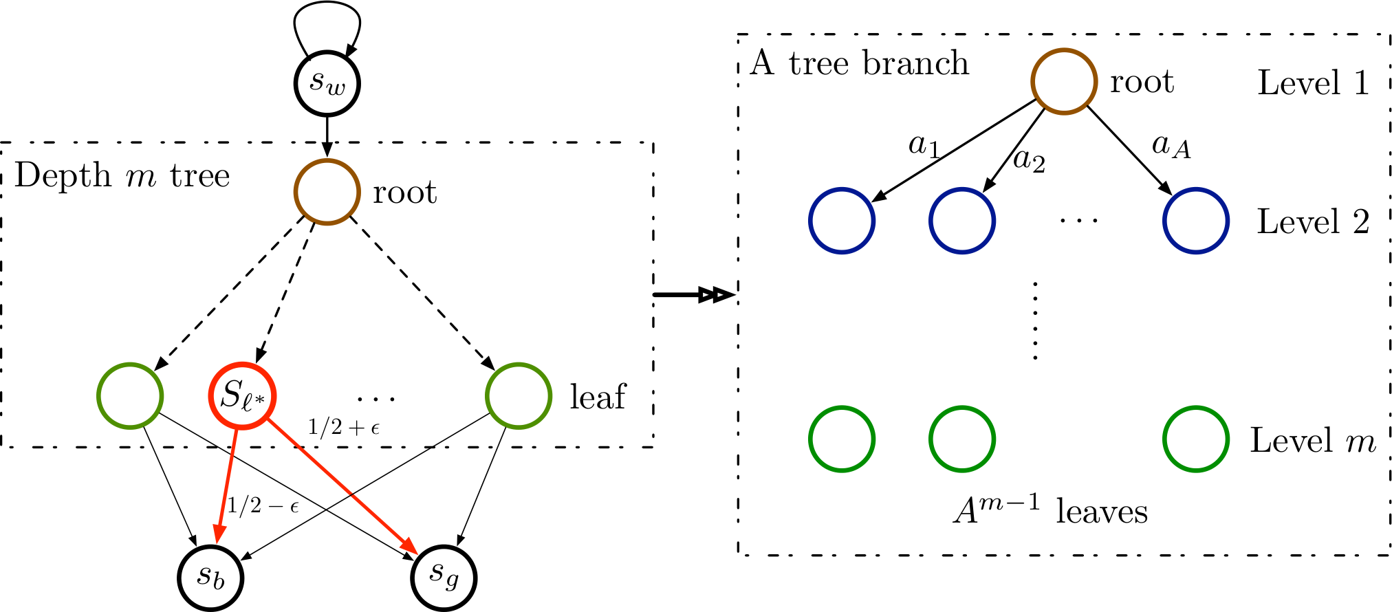
In the sequel, we assume that the depth of the tree is and , i.e., the depth tree is saturated. We further assume that the horizon . These assumptions simplify the presentation and can be removed as shown in Appendix D of Domingues et al. 2021. We define the reward to be zero on all states except ; on , it holds that
The transition probability at follows
In words, only transits to and . The special action allows the state to stay at for steps. After that, one must transits from to .
In the tree, the transition is deterministic and one can only move downwards in the tree. That is, traveling from the root to a leaf takes steps. We use to index the leaf states. Assume is a triple of special time, leaf and action, where . Then the transition from a leaf state to and is totally random except at leaf with action , i.e.,
where is a small probability to be determined later. The transition to and says that at some time , there is a special leaf with action that enables slightly increased probability to reach the “good” state . Therefore, finding the optimal policy is equivalent to identifying . We shall take uniformly random.
Lower bound analysis
Leveraging the insights from Proposition 4.6, the optimal policy with -step delay is the same as no delay, since the transition in the constructed instance is deterministic except for and . To this end, we can apply the analysis in Theorem 9 of Domingues et al. 2021 with the substitution of their to , and , respectively. Following Equation (12) in Domingues et al. 2021 and taking , we obtain
where is the number of leaves and can be rewritten as . By the assumption of and , we deduce
∎
Appendix C Omitted proofs in Section 5
C.1 Proof of Proposition 5.1
Proof.
We first show that the ground-truth transition probabilities belongs to with high probability. By Theorem 2.2 in Weissman et al. 2003 (see also Equation (44) in Jaksch et al. 2010), at the -th episode, for any fixed , we have
Setting for some constant ensures that
holds over any with probability . As a consequence, the event holds with probability over all .
Conditioned on the high probability event for all , we have by standard performance difference arguments that
where inequality follows from the valid optimism since Line 4 in Algorithm 3 is taken over double maximization, equality recursively expands the value function and denotes the inner product, inequality invokes Azuma-Hoeffding’s inequality, and inequality invokes Lemma C.2. ∎
C.2 Proof of Theorem 5.2
Proof.
The proof utilizes similar steps as Theorem 4.1, with extra care on the summation of bonus functions.
Valid optimism
We verify that the choice of bonus functions leads to a valid optimism.
Lemma C.1.
Given any failure probability , we set the bonus functions as
Then with probability , it holds that
Proof of Lemma C.1.
In the proof, we omit subscripts “aug” for simplicity. We use backward induction on time again. The base case of holds immediately due to the initial value of . Suppose the assertion holds at time . Then for time , if , the assertion holds trivially. Otherwise, we have
We lower bound terms and separately. For term , we have
In , is the pure state . We bound as
where inequality invokes Hoeffding’s inequality and holds with probability for any and some constant . Term is immediately bounded by
Putting and together, we derive
with high probabilty. For term , we have
Taking and summing up and , we have
We estimate by its empirical average. In episode , we have access to i.i.d. realizations of a Bernoulli random variable with rate (observable or not). Therefore, by Hoeffding’s inequality, we have
Substituting into and reloading constant sufficiently large give rise to
The proof is complete. ∎
Regret analysis
Summation of counting numbers
The summation over is standard. Using Azuma-Hoeffding’s inequality, we have
It remains to find the summations involving . First, we show that the event , i.e., the maximal consecutive delay is upper bounded by , holds with high probability. We have
since is a uniform lower bound on . Next, we provide an upper bound on . For a given tuple , the consecutive missing length is . Such a missing pattern appears with probability at most . As a consequence, denote as the number of consecutive missings in episodes. With probability , we have
by Bernstein’s inequality in Lemma D.1. Furthermore, at a fixed time , we use Lemma C.3 to bound the gap between two consecutive appearances of the same missing pattern. We instantiate Lemma C.3 with and obtain that the gap is bounded by with probability . Within the gap, the number of consecutive delays of length larger than is bounded by
where inequality follows from Bernstein’s inequality again and inequality invokes the fact for and bounds by . Now we can bound the summation of the counting numbers. Conditioned on the event , we have
where inequality follows since is repeated at most times before getting an update and inequality follows from the Cauchy-Schwarz inequality, and inequality invokes the assumption . Moreover, conditioned on the event , we also have
Combining the above
On event , the regret is bounded by
where is a sufficiently large constant and we substitute the bonus functions into inequality .
On the complement of , the regret is bounded by . We choose such that . We can now check that . Therefore, combining the regret on event and the complement event leads to
The proof is complete. ∎
C.3 Supporting Lemmas
Lemma C.2.
Suppose Assumption 2.2 holds. With probability for some failure probability , we have
Proof of Lemma C.2.
For any time , we denote as the collection of episodes that the -th and -th step observations are available. It is clear that the cardinality of is bounded by for any . Within each , we would like to bound the gap between two observations. Thanks to Lemma C.3, the gap is bounded by with probability . We set , which implies . Therefore, for any time step , available observations are at most separated by episodes.
With this notation, we bound
where inequality follows since will only be updated when and then repeat at most times, inequality invokes the cardinality bound on , and inequality follows from the standard pigeon-hole principle. ∎
Lemma C.3.
Let be i.i.d. Bernoulli random variables. Suppose . Define the largest gap between ’s as
Then for any integer , the following tail probability bound holds,
Proof of Lemma C.3.
We denote as the index set for when . Let , which is a geometric random variable with a success rate . Note that the cardinality of is at most . Therefore, we have
where the last inequality follows from . ∎
Appendix D Helper concentration inequalities
Lemma D.1 (Bernstein’s inequality).
Let be i.i.d. zero mean random variables. Suppose for any . Then for all positive , it holds that
In particular, given a failure probability , it holds that
Proof of Lemma D.1.
The proof of Bernstein’s inequality is standard, see for example (Wainwright 2019, Section 2.1). Here we verify the second claim. Let hold true. We find a suitable by
It is enough to choose . ∎
Lemma D.2 (Hoeffding’s inequality).
Let be i.i.d. random variables. Suppose for any . Then for all positive , it holds that
In particular, given a failure probability , it holds that
Proof of Lemma D.2.
The proof is standard; see (Wainwright 2019, Section 2.1). ∎
Lemma D.3 (Azuma-Hoeffding’s inequality).
Let be a martingale adapted to a filtration . Suppose and . Then for all positive , it holds that
In particular, given a failure probability , it holds that