Towards Fair Disentangled Online Learning for Changing EnvironmentsConference: Proceedings of the 29th ACM SIGKDD Conference on Knowledge Discovery and Data Mining; August 6–10, 2023; Long Beach, CA, USAProceedings of the 29th ACM SIGKDD Conference on Knowledge Discovery and Data Mining (KDD ’23), August 6–10, 2023, Long Beach, CA, USAPrice: 15.00DOI: 10.1145/3580305.3599523ISBN: 979-8-4007-0103-0/23/08CCS: Computing methodologies Artificial intelligenceCCS: Computing methodologies Machine learningCCS: Applied computing Law, social and behavioral sciencesCCS: Social and professional topics User characteristics

In online learning, data batches $\mathcal{D}_{t}$, defined as tasks, arrive one after another over time. An online machine learner can learn from new information in real-time as they arrive. Specifically, at each time, the learner faces a loss function $f_{t}:\mathbb{R}^{d}\times\Theta\rightarrow\mathbb{R}$ which does not need to be drawn from a fixed distribution and could even be chosen adversarially over time (Finn et al. 2019). The goal of the learner over all times $T$ is to decide a sequence of model parameters $\{\boldsymbol{\theta}_{t}\}_{t=1}^{T}$ by an online learning algorithm, e.g., follow the leader (Hannan 1957), that performs well on the loss sequence $\{f_{t}(\mathcal{D}_{t},\boldsymbol{\theta}_{t})\}_{t=1}^{T}$. Particularly, to evaluate the algorithm, a standard objective for online learning is to minimize some notion of regret, defined as the overall difference between the learner’s loss $\sum\nolimits_{t=1}^{T}f_{t}(\mathcal{D}_{t},\boldsymbol{\theta}_{t})$ and the best performance achievable by comparators.

Static regret. In general, one assumes that tasks collected over time are sampled from a fixed and stationary environment following the i.i.d assumption. Therefore, with a sequence of model parameters learned from the learner, the objective is to minimize the accumulative loss of the learned model to that of the best fixed comparator $\boldsymbol{\theta}\in\Theta$ in hindsight. This regret is typically referred to as static regret since the comparator is time-invariant.

The goal of online learning under a stationary environment is to design algorithms such that static regret $R_{s}$ sublinearly grows in $T$. However, low static regret does not necessarily imply a good performance in changing environment, where tasks are sampled from various distributions, since the time-invariant comparator $\boldsymbol{\theta}$ in Eq. 1 may behave badly. Tasks sequentially collected from non-stationary environments and distributions of them varying over time are more realistic. To address this limitation, recent advances (Zhang et al. 2017; Yang et al. 2016) have introduced enhanced regret metrics, i.e., dynamic regret, to measure the learner’s performance.

Dynamic regret. The dynamic regret (Zinkevich 2003) is defined as the difference between the cumulative loss of the learner and that of a sequence of comparators $\mathbf{u}_{1},\cdots,\mathbf{u}_{T}\in\Theta$.

In fact, Eq. 2 is more general since it holds for any sequence of comparators and thus includes the static regret in Eq. 1. Therefore, minimizing dynamic regret can automatically adapt to the nature of environments, either stationary or dynamic. However, distinct from static regret, bounding dynamic regret is challenging because one needs to establish a universal guarantee that holds for any sequence of comparators (Zhang et al. 2018). An alternative solution for this challenge is to bound the regret in terms of some regularities of the comparator sequence, e.g., path-length (Zinkevich 2003) defined in Eq. 9 which measures the temporal variability of the comparator sequence.

As alluded to in Section 1, most of the state-of-the-art online techniques ignore the significance of learning by being aware of model fairness, which is an important hallmark of human intelligence. To control bias, especially ensure group fairness across different sub-populations, cumulative fairness notions are considered as constraints added on regrets.

In general, group fairness criteria used for evaluating and designing machine learning models focus on the relationships between the sensitive variables and the system output (Zhao and Chen 2019; Wu et al. 2019; Zhao and Chen 2020). The problem of group unfairness prevention can be seen as a constrained optimization problem. For simplicity, we consider one binary sensitive label, e.g. gender, in this work. However, our ideas can be easily extended to many sensitive labels with multiple levels.

Let $\mathcal{P=X\times Z\times Y\times E}$ be the data space, where $\mathcal{X}\in\mathbb{R}^{d}$ is an input feature space, $\mathcal{Z}\in\{-1,1\}$ is a sensitive space, $\mathcal{Y}\in\{0,1\}$ is an output space for binary classification, and $\mathcal{E}\in\mathbb{N}$ denotes an environment space. Given a task $\mathcal{D}=\{(\mathbf{x}_{i},z_{i},y_{i},e_{i})\}_{i=1}^{n}\in\mathcal{P}$ in environment $e_{i}\in\mathcal{E}$, a fine-grained measurement to ensure group fairness in class label prediction is to design fair classifiers by controlling the notions of fairness between sensitive subgroups $\{z_{i}=1\}_{i=1}^{n_{1}}$ and $\{z_{i}=-1\}_{i=1}^{n_{-1}}$ where $n_{1}+n_{-1}=n$, e.g., demographic parity (Wu et al. 2019; Lohaus et al. 2020).

Notice that, in Eq. 3, when $\hat{p}_{1}=\mathbb{P}_{(\mathbf{x},z,y,e)\in\mathcal{P}}(z=1)$, the fairness notion $g(\mathcal{D},\boldsymbol{\theta})$ is defined as the difference of demographic parity (DDP). Similarly, when $\hat{p}_{1}=\mathbb{P}_{(\mathbf{x},z,y,e)\in\mathcal{P}}(y=1,z=1)$, $g(\mathcal{D},\boldsymbol{\theta})$ is defined as the difference of equality of opportunity (DEO) (Lohaus et al. 2020). Therefore, parameters $\boldsymbol{\theta}$ in the domain of a task are feasible if they strictly satisfy the fairness constraint $g(\mathcal{D},\boldsymbol{\theta})=0$.

Motivations. To tackle the problem of fairness-aware online learning in changing environments, a learner needs to update model parameters with a global change, which is costly and inefficient. Inspired by the sparse mechanism shift hypothesis (Schölkopf et al. 2021), we state changing environments in online learning can be attributed to partial changes in learned parameters in the long run that are specific to environments. This implies that some parameters remain semantically invariant across different environments.

We consider a general sequential setting where a learner is faced with tasks $\{\mathcal{D}_{t}\}_{t=1}^{T}$ one after another. Each of these tasks corresponds to a time, denoted as $t\in[T]$. At each time, the goal of the learner is to determine model parameters $\boldsymbol{\theta}_{t}$ using existing task pool $\{\mathcal{D}_{i}\}_{i=1}^{t-1}$ in a fair domain $\Theta$ that perform well for the task arrived at $t$. This is monitored by the loss function $f_{t}$ and the fairness notion $g_{t}$, wherein the fair constraint $g_{t}(\mathcal{D}_{t},\boldsymbol{\theta}_{t})=0$ is satisfied and $f_{t}(\mathcal{D}_{t},\boldsymbol{\theta}_{t})$ is minimized. To adapt to changing environments, crucially, model parameters $\boldsymbol{\theta}_{t}=\{\boldsymbol{\theta}_{t}^{s},\boldsymbol{\theta}_{t}^{v},\boldsymbol{\theta}_{t}^{d},\boldsymbol{\theta}_{t}^{cls}\}$ can be partitioned into multiple elements, specifically in which $\boldsymbol{\theta}_{t}^{s}$ captures the semantic information of data through a semantic encoder $h_{s}:\mathcal{X}\times\Theta\rightarrow\mathcal{S}$, and $\boldsymbol{\theta}^{cls}_{t}$ is used for prediction under fair constraints. $\boldsymbol{\theta}_{t}^{v}$ and $\boldsymbol{\theta}_{t}^{d}$ are parameters, later introduced in Sections 4.2 and 4.3, for encoding the environmental information and decoding latent representations, respectively, in order to adaptively train a good $\boldsymbol{\theta}^{s}_{t}$. For data batches sampled from heterogeneous distributions at different times, $\boldsymbol{\theta}^{s}_{t}$ corresponds to adapting to changing environments by encoding samples to a latent semantic space. With latent factors (representations) encoded from the semantic space as inputs, $\boldsymbol{\theta}^{cls}_{t}$ is time-invariant in the long run.

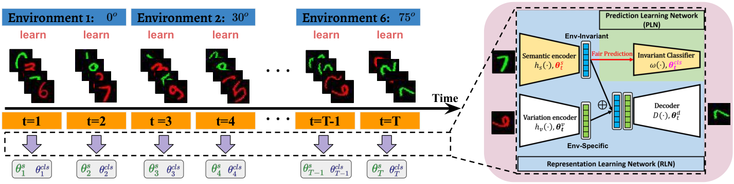
The overall protocol for this setting is as follows:

1. (1)

   The learner selects semantic parameters $\boldsymbol{\theta}^{s}_{t}$ and classification parameters $\boldsymbol{\theta}^{cls}_{t}$ in the fair domain $\Theta$.

2. (2)

   The world reveals a loss and fairness notion $f_{t}$ and $g_{t}$.

3. (3)

   The learner incurs an instantaneous loss $f_{t}(h_{s}(\mathcal{D}_{t},\boldsymbol{\theta}_{t}^{s}),\boldsymbol{\theta}^{cls}_{t})$ and fairness estimation $g(h_{s}(\mathcal{D}_{t},\boldsymbol{\theta}_{t}^{s}),\boldsymbol{\theta}^{cls}_{t})$.

4. (4)

   Advance to the next time.

As mentioned in Section 3.1, the goal of the learner is to minimize regret under long-term constraints (Mahdavi et al. 2012), defined as the summation of fair constraints over time. Since $\boldsymbol{\theta}^{s}_{t}$ adapts to different environments to encode semantic information from a latent invariant space and $\boldsymbol{\theta}^{cls}_{t}$ further takes semantic inputs for fair prediction, let $\{\boldsymbol{\theta}^{s}_{t},\boldsymbol{\theta}^{cls}_{t}\}_{t=1}^{T}$ be the sequence of parameters generated at the Step (1) of the protocol. We propose a novel fairness-aware regret for changing environments, namely FairSDR, defined as

where $[\cdot]_{+}$ is the projection onto the non-negative space. Similar to $\{\mathbf{u}_{1},\cdots,\mathbf{u}_{T}\}$ denoted in Eq. 2, $\{\mathbf{u}^{s}_{1},\cdots,\mathbf{u}^{s}_{T}\}$ are a sequece of semantic comparators to $\{\boldsymbol{\theta}^{s}_{1},\cdots,\boldsymbol{\theta}^{s}_{T}\}$, where each corresponds to an underlying environment. $\boldsymbol{\theta}^{cls}$ is the best-fixed comparator for fair classification, which is time-invariant.

Remarks. In contrast to the regret proposed in (Zhao et al. 2022) in which it is extended from the interval-based strongly adaptive regret, and it aims to minimize the maximum static regret for all intervals on the undivided model parameter, FairSDR takes the mixed form of static and dynamic regrets. Furthermore, (Zhao et al. 2022) employs the meta-learning framework in which the function inside $f_{t}$ is designed for interval-level learning with gradient steps on $\boldsymbol{\theta}$. However, in FairSDR, $h_{s}$ encodes an input to a semantic representation through a neural network on $\boldsymbol{\theta}^{s}$, which is part of $\boldsymbol{\theta}$.

Recall that in the learning protocol mentioned in Section 4.1, the main goal for the learner is to generate the parameter sequence $\{\boldsymbol{\theta}^{s}_{t},\boldsymbol{\theta}^{cls}_{t}\}_{t=1}^{T}$ in Section 4.1 that performs well on the loss sequence and the long-term fair constraints. We make the following assumptions.

This assumption is closely related to the shared latent space assumption in (Liu et al. 2017), wherein (Liu et al. 2017) assumes a fully shared latent space. We postulate that only the semantic space can be shared across environments whereas the variation factor is environment specific, which is a more reasonable assumption when the cross-environment mapping is many-to-many. In other words, given datapoints in various environments, each can be encoded into semantic and variation factors within the same semantic space but with different variation factors depending on the environments.

Under 1, each datapoint is able to be disentangled with semantic and variation factors. With two datapoints sampled from the same environment $e_{i}$, given a decoder $D:\mathcal{S}\times\mathcal{V}\times\Theta\rightarrow\mathcal{X}$, we assume that

2 enforces the data invariance of the original input $\mathbf{x}_{i}$ and the one that $D(h_{s}(\mathbf{x}_{i},\boldsymbol{\theta}^{s}),h_{v}(\mathbf{x}_{j},\boldsymbol{\theta}^{v}),\boldsymbol{\theta}^{d})$ reconstructs jointly from semantic and variation latent factors when the latter remains but the former varies.

This assumption shows that the prediction depends only on the semantic factor $h_{s}(\mathbf{x},\boldsymbol{\theta}^{s})$ regardless of the variation factor $h_{v}(\mathbf{x},\boldsymbol{\theta}^{v})$. Furthermore, the semantic factors are used for fair prediction under fairness constraints.

As the motivation stated in Section 3, an efficient online algorithm is expected to partially update model parameters (i.e., $\boldsymbol{\theta}^{s}_{t}$) to adapt to changing environments sequentially and to remain the rest (i.e., $\boldsymbol{\theta}^{cls}_{t}$). As the illustration shown in Fig. 1, a novel online framework for changing environments is proposed with two separate networks. The representation learning network (RLN) aims to learn a good semantic encoder $h_{s}$ that is able to accurately disentangle semantic representations within various environments, associated with the variation encoder $h_{v}$ and the decoder $D$. The prediction learning network (PLN) solely consists of the classifier $\omega$ and it takes semantic representations from RLN and outputs fair predictions under fair constraints, which is invariant to environments.

Specifically in RLN, to learn a good semantic encoder $h_{s}$, at each time $t$ we consider a data batch $\mathcal{Q}_{t}=\{(\mathbf{r}_{1,q,t},\mathbf{r}_{2,q,t},\mathbf{r}_{3,q,t},\mathbf{r}_{4,q,t})\}_{q=1,t}^{Q}$ containing multiple quartet data pairs sampled from existing task pool $\{\mathcal{D}_{i}\}_{i=1}^{t-1}$, where $Q$ denotes the number of quartet pairs in $|\mathcal{Q}_{t}|$.

• •

  $\mathbf{r}_{1,q,t}=(\mathbf{x}_{a,t},z_{a,t},y_{t},e_{t})$ with class $y_{t}$ and environment $e_{t}$

• •

  $\mathbf{r}_{2,q,t}=(\mathbf{x}_{b,t},z_{b,t},y^{\prime}_{t},e_{t})$ with class $y^{\prime}_{t}$ and environment $e_{t}$

• •

  $\mathbf{r}_{3,q,t}=(\mathbf{x}_{c,t},z_{c,t},y_{t},e^{\prime}_{t})$ with class $y_{t}$ and environment $e^{\prime}_{t}$

• •

  $\mathbf{r}_{4,q,t}=(\mathbf{x}_{d,t},z_{d,t},y^{\prime}_{t},e^{\prime}_{t})$ with class $y^{\prime}_{t}$ and environment $e^{\prime}_{t}$

Notice that $\mathbf{r}_{1,q,t}$ and $\mathbf{r}_{2,q,t}$ (same to $\mathbf{r}_{3,q,t}$ and $\mathbf{r}_{4,q,t}$) share the same environment label $e_{t}$ but different labels $y_{t}$ and $y^{\prime}_{t}$. $\mathbf{r}_{1,q,t}$ and $\mathbf{r}_{3,q,t}$ (same to $\mathbf{r}_{2,q,t}$ and $\mathbf{r}_{4,q,t}$) share the same label $y_{t}$ but different environments $e_{t}$ and $e^{\prime}_{t}$. We view $\mathbf{r}_{3,q,t}$ ($\mathbf{r}_{4,q,t}$) is an alternative pair to $\mathbf{r}_{1,q,t}$ ($\mathbf{r}_{2,q,t}$) with changing environments. For simplicity, we omit the subscripts $q$ and $t$.

Under 2, for $(\mathbf{r}_{1},\mathbf{r}_{2})$ and $(\mathbf{r}_{3},\mathbf{r}_{4})$ within the same environment but different labels, the data reconstruction loss $\mathcal{L}_{recon}$ is given:

where $\mathbf{s}_{a}=h_{s}(\mathbf{x}_{a},\boldsymbol{\theta}_{t}^{s})$, $\mathbf{s}_{c}=h_{s}(\mathbf{x}_{c},\boldsymbol{\theta}_{t}^{s})$, $\mathbf{v}_{b}=h_{v}(\mathbf{x}_{b},\boldsymbol{\theta}_{t}^{v})$, and $\mathbf{v}_{d}=h_{v}(\mathbf{x}_{d},\boldsymbol{\theta}_{t}^{v})$. $dist:\mathcal{X}\times\mathcal{X}\rightarrow\mathbb{R}$ indicates a distance metric, where we use $\ell_{1}$ norm in the experiments.

Similarly, under 3, for $(\mathbf{r}_{1},\mathbf{r}_{3})$ and $(\mathbf{r}_{2},\mathbf{r}_{4})$ with the same label but different environments, the class invariance loss $\mathcal{L}_{inv}$ is given:

where $\mathbf{x}_{a\rightarrow c}=D(\mathbf{s}_{a},\mathbf{v}_{c},\boldsymbol{\theta}_{t}^{d})$, $\mathbf{x}_{b\rightarrow d}=D(\mathbf{s}_{b},\mathbf{v}_{d},\boldsymbol{\theta}_{t}^{d})$, and $\ell_{CE}:\mathbb{R}\times\mathbb{R}\rightarrow\mathbb{R}$ is the cross-entropy loss function.

Finally, to ensure prediction accuracy within a fair domain, we combine $(\mathbf{r}_{1,q},\mathbf{r}_{2,q},\mathbf{r}_{3,q},\mathbf{r}_{4,q})$ together over the batch $\mathcal{Q}_{t}$ to estimate $\mathcal{L}_{cls}$ and $\mathcal{L}_{fair}$:

where $\oplus$ denotes concatenation operator between $\boldsymbol{\theta}_{t}^{s}$ and $\boldsymbol{\theta}_{t}^{cls}$.

In practice, requirements for remaining data invariance for datapoints sampled in the same environment with different labels and for keeping class invariance for datapoints sampled with the same label within various environments are hard to be satisfied. Similar to the fairness constraint, it is a strict equality constraint that is difficult to enforce in practice. To alleviate some of such difficulties, we relax the loss functions with empirical constants that

$\epsilon_{1},\epsilon_{2},\epsilon_{3}>0$ are fixed margins that control the extent to violations.

Furthermore, we propose a primal-dual Algorithm 1 for efficient optimization, wherein it alternates between optimizing $\boldsymbol{\theta}_{t}=\{\boldsymbol{\theta}_{t}^{s},\boldsymbol{\theta}_{t}^{v},\boldsymbol{\theta}_{t}^{d},\boldsymbol{\theta}_{t}^{cls}\}$ at each time via minimizing the empirical Lagrangian with fixed dual $\lambda_{t}=\{\lambda_{t,1},\lambda_{t,2},\lambda_{t,3}\}$ corresponding for $\mathcal{L}_{fair}$, $\mathcal{L}_{recon}$ as well as $\mathcal{L}_{inv}$ and updating the dual variable according to the minimizer (lines 24-32). The primal-dual iteration has clear advantages over stochastic gradient descent in solving constrained optimization problems. Specifically, it avoids introducing extra balancing hyperparameters. Moreover, it provides convergence guarantees once we have sufficient iterations and a sufficiently small step size (Zhang et al. 2022).

Moreover, because each task corresponds to a timestamp $t$ and an unknown environment before $\mathcal{D}_{t}$ arrives, the collected task pool $\{\mathcal{D}_{i}\}_{i=1}^{t-1}$ may be sampled from a single environment. In this sense, instead of using a batch stated in Section 4.3 with multiple quartet pairs, a sampled batch with doublet pairs containing $\{(\mathbf{r}_{1,q,t},\mathbf{r}_{1,q,t})\}_{q=1,t}^{Q}$ is considered. As a consequence, the class invariance loss in Eq. 5 is set to zero (lines 17-20).

As shown in the first three columns in Fig. 3, model performance is sequentially evaluated by fairness metrics (i.e., DP, EO, and MD) introduced in Section 6. Our results demonstrate FairDolce outperforms baseline methods by giving the highest DP and EO values and the lowest MD overall. Specifically, it eventually meets the fair criteria of "80%-rule" (Biddle 2005) where DP and EO at the last several times are beyond 0.8. The last column of Fig. 3 shows the change of model accuracies over time. We claim that FairDolce substantially outperforms alternative approaches with robust performance under dynamic environments in achieving the highest accuracy of all time.

As a tough competitor, FairSAOML addresses the same problem that we stated in this paper by proposing an expert-tracking technique in which experts’ weights are updated accordingly. It assumes that larger experts containing information across a large number of tasks help the learner to adapt to the new environment quickly. In our experiments, although FairSAOML shows competitive performance in bias control, it cannot surpass ours. This is because when the environment changes, larger experts in FairSAOML retain information from the old environments, which hurts the performance of the learner. Similar reasons are attributed to interval-based learning algorithms, such as AOD and CBCE. In the case of changing environments, one major merit of FairDolce is to disentangle data by separated representations in latent spaces, where only the semantic ones correspond to model predictions. This effectively controls the interference from various environments.

We conduct ablation studies on all datasets to demonstrate the contributions of three key components in our method. Fig. 4 demonstrates the results on the rcMNIST dataset. Results on other datasets refer to Figs. 5, 6 and 7 in Appendix B. (1) In this first study ($w/o\>h_{v}\>\&\>D$), we intentionally remove the variation encoder $h_{v}$ and the decoder $D$ and only keep the semantic encoder $h_{s}$ and the classifier $\omega$ with fair constraints. In this sense, the proposed architecture is equivalent to a simple neural network, and the semantic encoder functions as a featurizer. (2) In the second study ($w/o\>\text{fair constraints}$), we keep all modules but remove the fairness constraints $g$ from the classifier $\omega$. Without fair constraints, although the model provides better performance, fairness is not guaranteed over time. (3) In the third study ($w/o\>h_{v}$), only the variation encoder $h_{v}$ is removed. Without the variation encoder, the model is similar to conventional auto-encoders. The generalization ability to changing environments is weakened.