Geometrically frustrated self-assembly of hyperbolic crystals from icosahedral nanoparticles
Abstract
Geometric frustration is a fundamental concept in various areas of physics, and its role in self-assembly processes has recently been recognized as a source of intricate self-limited structures. Here we present an analytic theory of the geometrically frustrated self-assembly of regular icosahedral nanoparticle based on the non-Euclidean crystal formed by icosahedra in hyperbolic space. By considering the minimization of elastic and repulsion energies, we characterize prestressed morphologies in this self-assembly system. Notably, the morphology exhibits a transition that is controlled by the size of the assembled cluster, leading to the spontaneous breaking of rotational symmetry.
I Introduction
Geometrically frustrated assembly, the assembly of building blocks that don’t “fit together”, has become a rich and actively-growing area of both theoretical and experimental research, due to its potential of assembling controllable self-limited assemblies with high complexity, with potential applications in areas from metamaterials, micro-robotics, to biomedical engineering Sadoc and Mosseri 1999; Bruss and Grason 2012; Irvine et al. 2010; Grason 2016; Lenz and Witten 2017; Travesset 2017; Haddad et al. 2019; Sadoc et al. 2020; Li et al. 2020; Meiri and Efrati 2021; Serafin et al. 2021; Hall et al. 2023; Hackney et al. 2023. Compared to traditional self-assembly systems producing ordered crystalline structures, these geometrically frustrated assembly systems open a new area with unprecedented possibilities.
Various modes of geometric frustration have been studied in the context of geometrically frustrated assemblies, from disk packings on curved surfaces Irvine et al. 2010; Modes and Kamien 2007, chiral twisted bundles Bruss and Grason 2012; Grason 2016, topological defects of liquid crystals Ackerman and Smalyukh 2017, and polygons/polyhedra which don’t tessellate Euclidean space Lenz and Witten 2017; Serafin et al. 2021; Schönhöfer et al. 2023, yielding a rich set of morphologies and properties. In particular, a new theory was proposed in Ref. Serafin et al. 2021 where non-Euclidean crystals, the ordered ideal tessellation of polygons and polyhedra at volume fraction in non-Euclidean space, can be used as reference states to explain and potentially predict the self-assembly of geometrically frustrated building blocks in Euclidean space. This theory has been developed for non-Euclidean crystals in positively curved space: the 3-sphere, , which applies to the self-assembly of tetrahedra and potentially also dodecahedra and octahedra.
In this paper we extend this theory of non-Euclidean crystal assembly to negatively curved space—three dimensional (3D) hyperbolic space, , and reveal new mathematical structures and resulting stressed morphologies of the assemblies. In particular, we choose charged regular icosahedral nanoparticles (NPs) as our model system. This choice is guided by the following facts. (i) Among of the five regular polyhedra in Euclidean 3D space (tetrahedron, cube, octahedron, dodecahedron, icosahedron), icosahedron only has regular tesselations in . All other polyhedra have tesselations in both and (depending on the number of polyhedra meeting at each edge). (ii) NPs are versatile self-assembly systems and it has been shown that highly regular icosahedral NPs can be obtained experimentally Hofmeister 1998; De Nijs et al. 2015. Following a setup similar to that of Ref. Serafin et al. 2021 we consider the self-assembly of icosahedral NPs driven by short-ranged attractive interaction and screened electrostatic repulsion. The short-ranged attraction includes both Van der Waals interactions and ligand binding. We also consider the the surface energy of the assembled clusters to be low Yan et al. 2019. With these assumptions, the NPs tends to form low dimensional structures with morphologies determined by the competition of stress from the geometric frustration and electrostatic repulsion. We show that the hyperbolic crystal , which is the lowest stress regular tessellation of icosahedra in , provides us with a reference metric of the stress-free state of the icosahedral NPs, characterizing the ground state of the NPs at low temperature (which lies only in ). We then consider a slice of this non-Euclidean crystal in Euclidean space , where an energy functional can then be defined using this reference metric, which corresponds to the energy cost by deforming the slice of the non-Euclidean crystal into Euclidean space. We then show how different types of morphologies arise from this geometrically frustrated self-assembly at different choices of parameters. In particular, we find that there is a transition from spherical to cylindrical shells, controlled by the radius of the assembled disk. Rotational symmetry spontaneously breaks at this transition.
This theory, developed based on icosahedral NPs, is applicable to general geometrically frustrated self-assembly systems where the stress-free tessellation can be realized in . The general mode of geometric frustration, where “extra volume” or “overlap” is isotropically generated as the building blocks bind, is partially released by having thin sheets with gaussian curvatures. We expect this theory to provide guiding principles for future studies of geometrically frustrated assembles characterized by negatively curved non-Euclidean crystal tessellations, which have been predicted to carry exotic excitations Kollár et al. 2019; Maciejko and Rayan 2021; Yu et al. 2020; Cheng et al. 2022; Maciejko and Rayan 2022; Urwyler et al. 2022; Bzdušek and Maciejko 2022.
II Results
II.1 Constructing the hyperbolic crystal {3,5,3}
We start by considering the packing of identical regular icosahedra in space. The dihedral angle between two adjacent faces in a regular icosahedron is , three icosahedra sharing a common edge would have a slight overlap of (Fig. 1a). This overlap can be eliminated by introducing negative curvature, i.e., putting the packing in , which is an isotropic 3D space with constant negative curvature. One way to intuitively understand this is by realizing that negative curvature can enlarge the space because a sphere of radius has volume proportional to in instead of in . Therefore, negatively curved space can accommodate more volume, making it possible to have 3 icosahedra sharing a common edge without overlap.
Among all crystals that can be tessellated by icosahedra, the hyperbolic crystal {3,5,3} is the “least frustrated”, meaning that the it corresponds to has the smallest negative curvature (Fig. 1c). The notion of {3,5,3} follows the Schläfli symbol for regular tessellations, where one starts with regular polyhedra with -sided regular polygons meet at each vertex, and fits these polyhedra together such that of them meet around each edge, forming the tessellation.
As detailed in App. A and B, we construct the {3,5,3} non-Euclidean crystal by mirror reflections starting from the fundamental domain of the icosahedron, following the Coxeter group Coxeter and Coxeter 1999. The resulting crystal is infinitely large. To perform calculations and visualize the results, we adopt the Poincaré ball model for (detailed in App. C). The Poincaré ball is an open unit ball in together with the metric
| (1) |
From this metric it is clear that distances between points close to the boundary of the Poincaré ball diverges, bringing points at in to this unit ball. In the Poincaé ball model, a geodesic (i.e., a length-minimizing curve between two points) is an arc perpendicular to the boundary of the unit ball, and a hyperplanes (i.e., surfaces with constant negative curvature that can be decomposed into disjoint union of geodesics) are spheres perpendicular to the boundary of the unit ball (Fig.1b).
The hyperbolic tiling {3,5,3} can be constructed via hyperbolic reflections, similar to how Euclidean crystals can be generated by mirror reflections in Euclidean space. First, construct a hyperbolic icosahedron (i.e., a polytope in with 20 faces having the same symmetry as icosahedron in Euclidean space) centered at the origin. The curvature of this is chosen such that the dihedral angle between two adjacent faces is (Fig. 1c). Then, reflect the central icosahedron using its 20 faces, we get the second layer of icosahedron. Repeating this process we get the entire tiling (Fig. 1c, and as detailed in App. B).

II.2 Model energy of frustrated NP self-assembly
We next consider the energy of the assemblies as one “flattens” the non-Euclidean crystal {3,5,3} to our Euclidean space. We consider a model energy of four parts Serafin et al. 2021,
| (2) |
Here describes the binding energy between the NPs, describes the exposed surfaces of the NPs in contact with the solvent. We consider the regime where is large (e.g., between a pair of bound NPs), and thus tight face-to-face binding following the pattern of the {3,5,3} non-Euclidean crystal is favored. Therefore, we can assume the assembly is obtained by choosing a suitable slice of the hyperbolic crystal , and flattening it into the Euclidean space. Once is chosen, and are fixed, as is determined by the amount of surfaces exposed to the solution and depends on the number of attached surfaces.
The morphology of in our Euclidean space is determined by the combination of and . We take the continuum limit to enable an analytic treatment of the problem. The elastic energy comes from the fact that the {3,5,3} non-Euclidean crystal necessarily needs to be distorted to fit into . Let be the actual Euclidean metric of the assembly and be the curved metric of representing the ideal, stress-free distance between the NPs. In the continuum theory, close to a local minimum the elastic energy can be generally written as that of an isotropic homogeneous elastic medium of Lamé coefficients ,
| (3) |
where is the volume element in , is the strain tensor defined as
| (4) |
where and can not be equal as the former is a curved metric and the later is a flat metric. Hence, stress necessarily develops in the self-assembly process.
The energy characterizes electrostatic repulsion between these charged NPs, using screened Coulomb potentials,
| (5) |
Since and are determined by the part we choose in the non-Euclidean crystal , and are determined by how this part is embedded in the Euclidean space. We minimize the total energy in two steps. First, we determine the appropriate part . Second, we numerically minimize the repulsion and elastic energy in the space of all possible morphologies of .
II.3 Choosing a slice of and the thin shell expansion
In general, choosing the right slice from the non-Euclidean crystal to predict the self-assembly in Euclidean space is a highly nontrivial question, as the real self-assembly process is out of equilibrium with complex kinetic pathways that determine the assemblies.
As a simple model, we consider a smooth 2D slice which has zero gaussian curvature in . The general theory we present here, in terms of constructing the non-Euclidean crystal and minimizing the model energy, is applicable to other choices of the slice. The choice of we take here is guided by the following considerations. First, given the electrostatic repulsion and the low surface energy, the NPs prefer to form 2D structures. Second, for the scalability of the assembly process, the 2D structure should have constant Gaussian curvature (otherwise pieces of this sheet can’t merge). This gives us three cases: 2D surface with constant negative, positive or zero Gaussian curvature, all cut from the non-Euclidean crystal .
For surface with constant negative Gaussian curvature, the area of a disk of radius is proportional to . Embedding such a surface into Euclidean space would cost too much elastic energy since the area a disk of radius in Euclidean space only grows as . Hence, such a surface is not energetically preferred. There are two types of surfaces with zero Gaussian curvature: surfaces equidistant to a geodesic and horospheres (Fig. 2a and b). Horospheres are all spheres tangent to the boundary of the Poincaré ball when viewed in the Poincaré ball model. These two surfaces give us the same continuous theory when the number of icosahedra is large (see App. D). Hence we only consider the horosphere. For surfaces with constant positive Gaussian curvature, after a hyperbolic translation, they can be thought of as spheres centered at origin. However, the curvature of such a sphere decays exponentially as a function of its radius. The theory thus essentially reduces to the zero Gaussian curvature case (see App. D) when we consider a large surface where the continuum theory is appropriate.


We next formulate a mathematical description of a horosphere for this problem. To do this, we first use the following coordinate system to parameterize the Poincaré ball,
| (6) | ||||
Here is the coordinate system (i.e., they label the icosahedra), and is the embedding of these points in , represented using the Poincaré ball model. Under this parameterization, any constant surface is a horosphere tangent to the boundary of the Poincaré ball at and the direction can be viewed as thickness direction of the horospheres. The coordinates are chosen such that they coincide with the stereographic projection of the horosphere at each given from the north pole to a plane normal to . The metric tensor under this coordinate system is
| (7) |
Because horospheres at different are equivalent (the Poincaré ball represents infinite ), without losing generality, we choose surface which passes through the center of the Poincaré ball as the center surface of and expand around ,
| (8) |
where the reference first and second fundamental form
| (9) |
It is worth noting that different choice of gives us different reference first and second fundamental form but they only differ by a scaling factor and don’t affect the embedding.
From the form of , it is clear that the reference in-plane metric of this horosphere is flat (as it is of zero Gaussian curvature), but the sheet expand/shrink at different heights across the normal direction, which is incompatible with the flat in-plane metric. This is the mode of geometric frustration in this problem.
This surface then intersect the icosahedra in the crystal, which will be the material in the assembly. Fig. 2d shows the icosahedra intersecting with the horosphere in the Poincaré sphere. It is worth noting that although in the figure it appears to be a finite sphere intersecting distorted icosahedra of different sizes, the actual picture of this assembly in is infinitely large, and all icosahedra are regular and identical, although they intersect the horosphere at different heights.
The intersection between the horosphere and the icosahedron edges are shown in Fig. 3a. These points have 5-fold rotational symmetries as the {3,5,3} tiling does. One interesting observation is that this pattern may be defined as a type of quasicrystal, which is new to our knowledge. This can be seen by doing a Fourier transform of the edge intersection pattern in Fig. 3a, which results in Fig. 3b. The sharp diffraction peaks and the 5-fold rotational symmetry, as well as the aperiodicity of the real space pattern, satisfies the criterion of “quasicrystals”. Distinct from known quasicrystals, some of which can be obtained by cutting a high dimensional (Euclidean) crystal using a low dimensional surface, this is obtained by cutting a non-Euclidean crystal using a 2D surface with no Gaussian curvature.
When the thickness is much smaller than the in-plane dimension of the surface and the radius of curvature (here we choose suitable unit of length such that the radius of curvature is one). We can apply thin shell approximation and the elastic energy density is
| (10) | ||||
where is the Young’s modulus, is the thickness, is the Poisson’s ratio, is the stretching energy density and is the bending energy density. The total elastic energy under this thin shell expansion is
| (11) |
Under the same thin shell approximation, the electrostatic repulsion energy can be written as,
| (12) |
where is the charge density, is the position of in the Euclidean space , and are area elements of around and respectively.
II.4 Minimizing the total energy and predicting the morphology
We next choose suitable parameters and computationally minimize for these thin shells. In the {3,5,3} tiling, the radius of the hyperbolic icosahedron is 0.88 (in unit of radius of curvature), slightly smaller than the radius of curvature. We choose to be a disk of radius ranging between 2 to 5 on the horosphere, reasonably greater than the radius of the hyperbolic icosahedron, so that the thin shell approximation is justified.
We numerically minimize (see App. E) of this thin shell. We have chosen the interaction parameters to be (thickness of the shell), (charge density), (inverse screening length), where is the radius of curvature of the hyperbolic space, and we have expressed the charge density in terms of the relative strength between the repulsion and the elasticity. These choices are guided by the requirement of making the elastic energy to be of the same order of magnitude of the repulsion energy, so that the balance of the two leads to nontrivial morphologies. The methods described here are not limited to this regime.
A series of morphologies we obtain at different disk sizes are shown in Fig. 4a-f. It is worth noting that although the reference fundamental forms and are rotationally symmetric, the final morphology can spontaneously break this symmetry. In particular, disks at small radius keep this symmetry, whereas larger disks become more cylinderical. This results from a crossover from bending dominated regime to stretching dominated regime as the radius of the disk becomes larger. Fig. 4g shows the deviation from rotational symmetric morphology as a function of radius. To quantify this effect, we introduce the following order parameter to measure the rotational symmetry breaking of the surface. For a given point on a surface , let be the normalized normal vector of the surface at . We first average over to find the rotation vector . Then we choose the rotation axis to be a line aligning with the rotation vector going through the mass center of the surface. Next, let be the the rotation operator about by angle , and we define the order parameter as
| (13) |
where is the area element of . When has rotational symmetry, is normal to everywhere, leading to . Nonzero captures how strongly the morphology breaks this symmetry.
Fig. 4h shows the morphology of the assembly when the icosahedra are explicitly shown. They are placed following their positions in the hyperbolic crystal, as discussed in App. E. Although these icosahedra are not in perfect face-to-face binding, our calculation shows that the assembly minimizes strain and repulsion by adopting this morphology.
III Conclusion
In this paper, we show that the self assembly of small cluster of charged icosahedral NPs under face-to-face attractive interaction and low surface energy can be understood using the hyperbolic crystal . By choosing zero-Gaussian curvature slices of the hyperbolic crystal and minimizing their energies in the Euclidean space, we find morphologies of these assembly, characterized by a transition where rotational symmetry breaks. We also find a possible new type of quasicrystal by cutting the hyperbolic crystal {3,5,3} using the horosphere.
This theory provides a new framework to employ non-Euclidean crystals beyond those residing in the 3-sphere, to predict the self-assembly of hyperbolic structures. These structures may be of interest both as new types of assemblies at the nanoscale, but also for emergent phenomena in hyperbolic space.
Acknowledgements— The authors acknowledge helpful discussions with Francesco Serafin, Nicholas Kotov, Sharon Glotzer, and Philipp Schönhöfer. This work was supported in part by the Office of Naval Research (MURI N00014-20-1-2479). X.M. acknowledges the hospitality of the Kavli Center for Theoretical Physics, supported by the National Science Foundation (NSF PHY-1748958), where this manuscript was completed.
Appendix A The hyperboloid model of hyperbolic space
In this section we review the hyperboloid model of hyperbolic space and hyperbolic reflections in the hyperboloid model Iversen 1992.
Let be a symmetric bilinear form on defined by
| (14) |
where
| (15) |
is the Minkowski metric tensor.
The hyperboloid model of hyperbolic space consists of a submanifold of
| (16) |
and a metric on induced by , where for any vector tangent to . The metric gives a distance function on satisfying
| (17) |
An isometry of is a smooth map preserving distance:
| (18) |
which is equivalent to
| (19) |
Form (19), we see that any linear map whose matrix under the standard basis of satisfying induces a smooth map
| (20) | ||||
and the induced map is an isometry. It turns out that the correspondence is bijective. In the following, we identify a matrix satisfying with an isometry of .
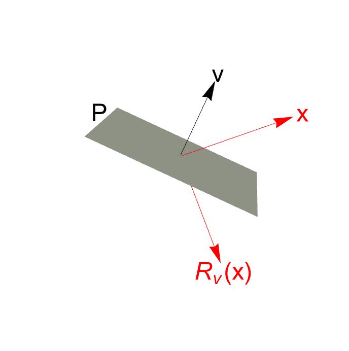
For any vector satisfying , consider the linear map
| (21) |
satisfies
| (22) |
Therefore, is an isometry of . Since we have
| (23) | ||||
can be viewed as a reflection about the hyperplane and such is called a hyperbolic reflection Iversen 1992. It is worth noting that a hyperbolic reflection can be identified with its normal vector or its reflecting plane .
Appendix B Constructing the {3,5,3} crystal in the hyperboloid model
In this section, we use hyperbolic reflections to construct hyperbolic crystal . There are three steps in the construction. First, construct a pyramid that is of one hyperbolic icosahedron in . Second, reflect by three of its four surfaces to form the central hyperbolic icosahedron . Third, reflect by its surfaces and we get the entire crystal.

We first construct the pyramid . Let be the four surfaces of , be the corresponding normal vectors under and be the corresponding hyperbolic reflections. In the tiling, satisfies
| (24) |
where
| (25) |
The corresponding vectors satisfies
| (26) |
’s are unique up to global rotations and we can take them to be
| (27) | ||||
Then we move by the group (a group of order 120) generated by to form the central hyperbolic icosahedron . The 20 surfaces of corresponds to reflections . Finally, we use the 20 surfaces of to reflect and get the entire crystal Coxeter and Coxeter 1999.
Appendix C The relation between the hyperboloid model and the Poincaré ball model
The hyperboloid model reviewed above is convenient for calculations of hyperbolic reflections, but the Poincaré ball model, which we use in the main text, is more convenient to visualize the hyperbolic space Iversen 1992. Here we review their relations.
The Poincaré ball model consists of an open unit ball
| (28) |
in and a metric
| (29) |
If we identify the Poincaré ball with , it is then related to the hyperboloid model projectively. If we have a point in the hyperboloid model, we may project it onto the hyperplane by intersecting it with a line drawn through . The result is the corresponding point of the Poincaré disk model. To put it explicitly, the projection sends to and is an isometry between and . Let be a hyperplane in and be a reflection in , then the corresponding hyperplane in is
| (30) |
and the corresponding reflection in the Poincaré ball model is given by
| (31) |
All constructions in the hyperboloid model carry over to constructions in the Poincaré ball model via (30) and (31).

Appendix D Reference fundamental forms of flat surfaces and spheres in hyperbolic space
In this section we calculate reference fundamental forms of spheres and surfaces equidistant to a geodesic in hyperbolic space, and show that both of them can be reduced to the case of horospheres discussed in the main text.
D.1 Spheres
Let be the hyperbolic radius of a hyperbolic sphere centered at the origin of the Poincare ball, in the Poincaré ball model. The sphere is described by . We use spherical coordinate to parametrize the sphere via
| (32) | ||||
The metric tensor under coordinate system is
| (33) |
The reference fundamental forms are
| (34) | ||||
In the large limit, near the equator
| (35) |
reducing to the horosphere case. Other parts of the sphere exhibit the same mode of geometric frustration given the rotational symmetry of the sphere, although they require a different choice of coordinate system to reduce to this particular form of the first and second reference fundamental forms.
D.2 Surfaces equidistant to a geodesic
A geodesic connecting points is the shortest curve joining . We choose a geodesic in the hyperboloid model. Let be the surface consisting of points in of distance to the geodesic . We can parametrize using coordinate by
| (36) | ||||
The metric tensor under coordinate system is
| (37) | ||||
The reference fundamental forms are
| (38) | ||||
In the large limit,
| (39) |
reducing to the horosphere case.
Appendix E Energy minimization and morphology of in Euclidean space
In this section, we show the minimization procedure of . For a disk of radius on the horosphere, since stereographic projection gives an isometry between the horosphere and a plane, the coordinates of the disk of radius in the horosphere form a disk of the same radius in Euclidean space. The geometric frustration, however, is reflected in the reference second fundamental form where the next layer (small increment of ) shrinks relative to the horosphere.
We triangulate the disk for computational minimization of the energy. For a given embedding from the nodes of the triangulation into , we use the method in reference Grinspun et al. 2006 to compute its fundamental forms and set , to calculate the elastic energy. We also put a total charge of (the coefficient is choosen so that the elastic energy is of the same order as the repulsion energy) on the entire disk, evenly distribute these charge to each node and use
| (40) |
to calculate the repulsion energy under the embedding . In this way, is a function of nodes positions in . we then do gradient descent with respect to nodes positions starting from many different initial configurations and pick the final configuration with minimal energy. After minimization, for radius we obtained the stretching energy , the bending energy and the elastic energy .
After obtaining the morphology of the mid-surface, we reconstruct the discrete assembly of icosahedra on using the following method. There are 31 icosahedra intersecting with the disk for the case of radius 5 and we project the centers of the 31 icosahedra onto the horosphere along the line, obtaining their corresponding coordinates and find these points ({}) on the embedding surface in . Then we calculate the hyperbolic distance between the centers of the 31 icosahedra to the horosphere respectively ({}). Next, we place Euclidean icosahedra of the same size as the hyperbolic icosahedra (in terms of the body-center to face-center distance) to the Euclidean space such that the icosahedron lies above/below the point on midsurface by distance . Finally, we rotate the icosahedra so that the overlapping among them is the smallest. The result is shown in Fig. 4h.
References
- Sadoc and Mosseri (1999) J.-F. Sadoc and R. Mosseri, Geometrical Frustration, Collection Alea-Saclay: Monographs and Texts in Statistical Physics (Cambridge University Press, 1999).
- Bruss and Grason (2012) I. R. Bruss and G. M. Grason, Proceedings of the National Academy of Sciences 109, 10781 (2012).
- Irvine et al. (2010) W. T. Irvine, V. Vitelli, and P. M. Chaikin, Nature 468, 947 (2010).
- Grason (2016) G. M. Grason, The Journal of Chemical Physics 145, 110901 (2016).
- Lenz and Witten (2017) M. Lenz and T. A. Witten, Nature physics 13, 1100 (2017).
- Travesset (2017) A. Travesset, Physical Review Letters 119, 115701 (2017).
- Haddad et al. (2019) A. Haddad, H. Aharoni, E. Sharon, A. G. Shtukenberg, B. Kahr, and E. Efrati, Soft Matter 15, 116 (2019).
- Sadoc et al. (2020) J.-F. Sadoc, R. Mosseri, and J. V. Selinger, New Journal of Physics 22, 093036 (2020).
- Li et al. (2020) C. Li, A. G. Shtukenberg, L. Vogt-Maranto, E. Efrati, P. Raiteri, J. D. Gale, A. L. Rohl, and B. Kahr, The Journal of Physical Chemistry C 124, 15616 (2020).
- Meiri and Efrati (2021) S. Meiri and E. Efrati, Physical Review E 104, 054601 (2021).
- Serafin et al. (2021) F. Serafin, J. Lu, N. Kotov, K. Sun, and X. Mao, Nature Communications 12, 4925 (2021).
- Hall et al. (2023) D. M. Hall, M. J. Stevens, and G. M. Grason, Soft Matter 19, 858 (2023).
- Hackney et al. (2023) N. W. Hackney, C. Amey, and G. M. Grason, arXiv preprint arXiv:2303.02121 (2023).
- Modes and Kamien (2007) C. D. Modes and R. D. Kamien, Physical review letters 99, 235701 (2007).
- Ackerman and Smalyukh (2017) P. J. Ackerman and I. I. Smalyukh, Physical Review X 7, 011006 (2017).
- Schönhöfer et al. (2023) P. W. Schönhöfer, K. Sun, X. Mao, and S. C. Glotzer, arXiv preprint arXiv:2305.07786 (2023).
- Hofmeister (1998) H. Hofmeister, Crystal Research and Technology: Journal of Experimental and Industrial Crystallography 33, 3 (1998).
- De Nijs et al. (2015) B. De Nijs, S. Dussi, F. Smallenburg, J. D. Meeldijk, D. J. Groenendijk, L. Filion, A. Imhof, A. Van Blaaderen, and M. Dijkstra, Nature materials 14, 56 (2015).
- Yan et al. (2019) J. Yan, W. Feng, J.-Y. Kim, J. Lu, P. Kumar, Z. Mu, X. Wu, X. Mao, and N. A. Kotov, Chemistry of Materials 32, 476 (2019).
- Kollár et al. (2019) A. J. Kollár, M. Fitzpatrick, and A. A. Houck, Nature 571, 45 (2019).
- Maciejko and Rayan (2021) J. Maciejko and S. Rayan, Science advances 7, eabe9170 (2021).
- Yu et al. (2020) S. Yu, X. Piao, and N. Park, Physical Review Letters 125, 053901 (2020).
- Cheng et al. (2022) N. Cheng, F. Serafin, J. McInerney, Z. Rocklin, K. Sun, and X. Mao, Physical Review Letters 129, 088002 (2022).
- Maciejko and Rayan (2022) J. Maciejko and S. Rayan, Proceedings of the National Academy of Sciences 119, e2116869119 (2022).
- Urwyler et al. (2022) D. M. Urwyler, P. M. Lenggenhager, I. Boettcher, R. Thomale, T. Neupert, and T. Bzdušek, Physical Review Letters 129, 246402 (2022).
- Bzdušek and Maciejko (2022) T. Bzdušek and J. Maciejko, Physical Review B 106, 155146 (2022).
- Coxeter and Coxeter (1999) H. Coxeter and H. Coxeter, The Beauty of Geometry: Twelve Essays, Dover books on mathematics (Dover Publications, 1999).
- Iversen (1992) B. Iversen, Hyperbolic Geometry, London Mathematical Society Student Texts (Cambridge University Press, 1992).
- Grinspun et al. (2006) E. Grinspun, Y. Gingold, J. Reisman, and D. Zorin, Computer Graphics Forum 25, 547 (2006), https://onlinelibrary.wiley.com/doi/pdf/10.1111/j.1467-8659.2006.00974.x .