Balanced Training of Energy-Based Models with Adaptive Flow Sampling

Louis Grenioux Affiliation: CMAP, CNRS, Ecole Polytechnique, Institut Polytechnique de Paris, 91120 Palaiseau, France Correspondence to: louis.grenioux@polytechnique.edu Éric Moulines Affiliation: CMAP, CNRS, Ecole Polytechnique, Institut Polytechnique de Paris, 91120 Palaiseau, France Correspondence to: eric.moulines@polytechnique.edu Marylou Gabrié Affiliation: CMAP, CNRS, Ecole Polytechnique, Institut Polytechnique de Paris, 91120 Palaiseau, France Correspondence to: marylou.gabrie@polytechnique.edu

Abstract

Energy-based models (EBMs) are versatile density estimation models that directly parameterize an unnormalized log density. Although very flexible, EBMs lack a specified normalization constant of the model, making the likelihood of the model computationally intractable. Several approximate samplers and variational inference techniques have been proposed to estimate the likelihood gradients for training. These techniques have shown promising results in generating samples, but little attention has been paid to the statistical accuracy of the estimated density, such as determining the relative importance of different classes in a dataset. In this work, we propose a new maximum likelihood training algorithm for EBMs that uses a different type of generative model, normalizing flows (NF), which have recently been proposed to facilitate sampling. Our method fits an NF to an EBM during training so that an NF-assisted sampling scheme provides an accurate gradient for the EBMs at all times, ultimately leading to a fast sampler for generating new data.

Keywords:

Energy-based models, Normalizing flows, MCMC, Sampling

1 Introduction

An Energy based model (EBM) defines a probability distribution over $x\in\mathcal{X}\subset\mathbb{R}^{d}$ by a parameterized energy function $E_{\theta}:\mathbb{R}^{d}\to\mathbb{R}$ with parameters $\theta\in\Theta$ as

p_{\theta}(x)=\frac{1}{Z_{\theta}}\exp\left(-E_{\theta}(x)\right)\,.

(1)

These conceptually simple models are very flexible, since the functional class of $E_{\theta}$ is unrestricted, provided that it must ensure that $\exp(-E_{\theta}(x))$ is integrable. However, this flexibility comes at the price of an unknown normalization constant $Z_{\theta}=\int\exp(-E_{\theta}(x))\mathrm{d}x$ , which is difficult to calculate in practice, and the lack of a simple sampling procedure for the model. As a result, it is difficult to train EBMs by maximum likelihood methods and to use them as generative models. To overcome these difficulties, various Monte Carlo Markov chains (MCMC) algorithms, from the simplest (e.g., (Hinton 2012)) to the most complicated (e.g., (Béreux et al. 2023)), as well as various variational inference methods (VI) (Welling & Hinton 2002; Gabrié et al. 2015; Dai et al. 2019; Grathwohl et al. 2021) were considered to approximate the likelihood gradients. Alternatively, weaker learning objectives have been proposed to avoid sampling $p_{\theta}(x)$ , including Score Matching (Hyvärinen 2005; Song & Ermon 2019), Noise Constrative Estimation (Gutmann & Hyvärinen 2010), and Minimum Stein Discrepancy (Grathwohl et al. 2020) - see (Song & Kingma 2021) for a recent methodological review of EBMs.

One of the main challenges common to all these training approaches is the correct estimation of the density of multimodal distributions, that is, datasets with several different clusters in the data. This is due to the difficulty for MCMCs and VIs to accurately represent multimodal distributions, or the difficulty for weaker learning objectives that rely on scores $\nabla_{x}\log p_{\theta}(x)$ to capture this information (see, e.g., (Song & Ermon 2019), Section 3.2.1). Meanwhile, the highly flexible parameterization of EBMs makes them particularly well suited to the multimodal setting, compared to the competing class of generative models parameterized as push-forward distributions, such as generative adversarial networks (GANs) or normalizing flows (NFs), whose ability to partition mass into multiple modes is inherently limited (Cornish et al. 2020; Salmona et al. 2022).

However, a number of recent works have shown that some generative push-forward models, namely NFs, facilitate the sampling of multimodal distributions (see references in Section 2). Building on these results, we propose joint learning of an EBM with a companion NF, which allows efficient sampling of the EBM at any point in the training and, as a result, accurate maximum likelihood training of the EBM. As described in the Related Work section, several proposals have already been made to combine EBMs with NFs. Our works goes a step further in this direction by employing a calibrated NF-assisted MCMC (Gabrie et al. 2022; Samsonov et al. 2022) recently shown to be particularly robust in the multimodal setting (Grenioux et al. 2023).

2 Background

EBM maximum likelihood training

Given a training data distribution $p^{\star}$ , the EBM log-likelihood can be written as $\ell_{\rm EBM}(\theta)=\mathbb{E}_{p^{\star}}[\log p_{\theta}(X)]$ . This quantity is intractable due to the unknown $Z_{\theta}$ of Equation 1, which translates into an expectation over $p_{\theta}$ in its gradient:

\nabla_{\theta}\ell_{\rm EBM}(\theta)=\mathbb{E}_{p^{\star}}[\nabla_{\theta}E_{\theta}(X)]-\mathbb{E}_{p_{\theta}}[\nabla_{\theta}E_{\theta}(X)].

(2)

A Monte-Carlo estimation of $\nabla_{\theta}\ell_{\rm EBM}(\theta)$ requires training samples $x^{(+)}_{i}\sim p^{\star}(x)$ , commonly referred to as positive samples in the EBM context, and samples from the current model $x^{(-)}_{i}\sim p_{\theta}(x)$ , respectively called negative samples. Collecting $n$ samples of these two kinds yields the approximation for gradient (2) $\widehat{\nabla_{\theta}\ell_{\rm EBM}}(\theta,\{x^{(-)}_{i},x^{(+)}_{i}\}_{i=1}^{n})=$

\displaystyle-\frac{1}{n}\left(\sum_{i=1}^{n}\nabla_{\theta}E_{\theta_{k}}(x^{(-)}_{i})-\sum_{i=1}^{n}\nabla_{\theta}E_{\theta_{k}}(x^{(+)}_{i})\right).

(3)

Yet, obtaining exact samples from $p_{\theta_{k}}$ requires converging an MCMC, which is a costly procedure to repeat. As a result, approximate sampling procedures have been proposed: in contrastive divergence (CD) (Hinton 2002), a fixed small number of MCMC steps is ran starting from training samples at each gradient computation. In persistent CD (PCD), this simple idea was further refined by propagating the MCMC chains the negative samples across gradient updates (Tieleman 2008). For real valued-valued EBMs, CD and PCD most commonly employ Uncalibrated Langevin Algorithm (ULA) (Roberts & Tweedie 1996), a local gradient-based sampler, which at step $k$ updates $x^{(k)}$ as

x^{(t+1)}=x^{(t)}-\eta\nabla\log E_{\theta}(x^{(t)})+\sqrt{2\eta}z^{(t)}\,

(4)

where $\eta$ is the step size of the algorithm and $z^{(t)}\sim\mathcal{N}(0,I)$ .

If ULA samples the target distribution $p_{\theta}$ asymptotically in time, it typically cannot converge in a manageable number of iterations for distribution that are multimodal. While recent research suggests that using a non-convergent MCMC for drawing negative samples does not compromise sample quality if a consistent sampling scheme is employed during and after training (Nijkamp et al. 2019; Nijkamp et al. 2020b; Nijkamp et al. 2020a; An et al. 2021; Xie et al. 2022), it is not guaranteed that an EBM trained in this fashion captures the overall mass distribution between different modes (see the motivating example of 4).

NF-Assisted sampling

Normalizing flows (NF) combine a base distribution $\rho$ on $\mathbb{R}^{d}$ and a bijective transport map $T_{\alpha}:\mathbb{R}^{d}\to\mathbb{R}^{d}$ with parameters $\alpha\in\mathbb{A}$ to define a generative model with density:

\displaystyle\lambda_{T_{\alpha}}^{\rho}(x)=\rho(T_{\alpha}^{-1}(x))\left\lvert J_{T_{\alpha}^{-1}}(x)\right\rvert,

(5)

from which samples are straightforwardly obtained as $X=T_{\alpha}(Z)$ with $Z\sim\rho$ . NFs can be trained on training data to maximize the explicit likelihood. We point the reader to the reviews (Papamakarios et al. 2021; Kobyzev et al. 2021).

Thanks to their tractable densities and direct sampling procedure, NFs have found applications in statistical inference either as a variational family (Rezende & Mohamed 2015; Wu et al. 2019) or as helpers in sampling algorithms (Parno & Marzouk 2018; Albergo et al. 2019; Noé et al. 2019; Müller et al. 2019; McNaughton et al. 2020; Hackett et al. 2021) (among others). Given a target distribution $\pi$ , known up to a normalization constant, the general idea of NF-assisted inference is to train the map $T_{\alpha}$ such that $\lambda_{T_{\alpha}}^{\rho}$ approaches $\pi$ . In this context, since no training sample is available a priori, the flow is trained either by minimizing the reverse Kulleback-Leibler (KL) divergence $\mathrm{KL}(\lambda_{T_{\alpha}}^{\rho}||\pi)=\mathbb{E}_{\lambda_{T_{\alpha}}^{\rho}}[\log\lambda_{T_{\alpha}}^{\rho}(x)/\pi(x)]$ (Rezende & Mohamed 2015) or through an adaptive MCMC procedure maximizing a proxy of the likelihood (Parno & Marzouk 2018; McNaughton et al. 2020; Naesseth et al. 2021; Gabrie et al. 2022). When $\pi$ is multimodal, the reverse KL is prone to mode collapse (Jerfel et al. 2021; Hackett et al. 2021), while the adaptive MCMC training can leverage prior knowledge of the different modes’ basins to seed the learning of a model covering all the regions of interest. Once trained, samples from the flow $\lambda_{T_{\alpha}}^{\rho}$ approximating the target $\pi$ can be debiased via importance sampling or various MCMC schemes. A recent comparative study (Grenioux et al. 2023) shows that methods based on independent proposals from the flow, such as independent Metropolis-Hastings (e.g., (Nicoli et al. 2020)), are more robust to sample multimodal distributions compared to re-parametrization schemes such as neutra-MCMC (Hoffman et al. 2019). In the context of EBM training, these observations suggest the use a of flow-based adaptive MCMC using independent proposals, FlowMC (Algorithm 5 in Appendix A), to provide accurate negative samples.

3 EBMs with Flow Sampling

Refer to caption — Figure 1: Comparison of PCD and flowMC EBM training on toy 2d mixture with 2:1 weight ratio. The EBM learned with flowMC (f) captured correctly the relative weights, unlike the EBM trained with ULA (b), as is also clear from the conditional densities along the axis going trough the centroids (d,h). This statistical accuracy is promoted by the fast mixing NF-assisted sampling (g). (Right) Estimated weight of the top right mode during the training of ULA-EBM and flowMC-EBM (Details in Section C.2)

We suggest to train a NF to maintain a good overlap between the flow’s $\lambda_{T_{\alpha}}^{\rho}$ and EBM’s $p_{\theta}$ throughout training so as to implement an NF-assisted sampler to draw negative samples (Algorithm 1). For this symbiosis to work in practice, that is $\lambda_{T_{\alpha_{t}}}^{\rho}\approx p_{\theta_{t}}^{\rho}$ at all times, we slightly modify the EBM definition Equation 1 using the flow base distribution $\rho$ as a tilt¹¹ 1 Note that this change does not modify the gradient of $\ell_{\rm EBM}(\theta)$ (see Equation 2) see proof in Appendix B.:

p_{\theta}^{\rho}(x)=\frac{1}{Z_{\theta}}\exp\left(-E_{\theta}(x)\right)\rho(x)\,.

(6)

Choosing initially $\theta_{0}$ such that $E_{\theta_{0}}(\cdot)=0$ and $\alpha_{0}$ such that $T_{\alpha_{0}}(\cdot)={\rm Id}(\cdot)$ leads to a perfect equality at initialization $p_{\theta_{0}}^{\rho}=\rho=\lambda_{T_{\alpha_{0}}}^{\rho}$ . Then, the learning rates $\gamma_{\rm EBM}$ and $\gamma_{\rm flow}$ in Algorithm 1 need to be co-adjusted for the matching to be approximately maintained all along.

Unlike strategies using ULA to obtain negative samples, our proposition is statistically reliable as it uses a calibrated MCMC sampler which handles multimodality. Thanks to the good agreement between $\lambda_{T_{\alpha_{t}}}^{\rho}$ and $p_{\theta_{t}}^{\rho}$ , non-local moves proposed by the NF in the flowMC sampler allow rapid-mixing between modes. This coupled learning of two generative models takes the best of both: the constrained but tractable NF approximates an unconstrained but intractable EBM. Additionally, it provides a natural and efficient way to sample the resulting EBM through FlowMC.

Algorithm 1 flowMC-EBM training step on data distribution

\rho^{\star}

with persistent initialization

Input: EBM parameter

\theta_{k}

, flow parameters

\alpha_{k}

, learning rates

\gamma_{\rm EBM}

and

\gamma_{\rm flow}

, batch size

n

, local step size

\eta

, number of MCMC steps

N

, persistent state

\{\tilde{x}_{i}\}_{i=1}^{n}

Output:

\theta_{k+1}

\alpha_{k+1}

, updated

\{\tilde{x}_{i}\}_{i=1}^{n}

1. Draw positive samples

\{x^{(+)}_{i}\}_{i=1}^{n}\sim\rho^{\star}

2. Draw negative samples from

p_{\theta_{k}}

using flow

T_{\alpha_{k}}

x^{(-)}_{i}=\mathrm{flowMC}(p_{\theta_{k}}^{\rho},\tilde{x}_{i},T_{\alpha_{k}},\rho,\eta,N)\text{ for all }i

3. Update the persistent state

\{\tilde{x}_{i}\}_{i=1}^{n}=\{x^{(-)}_{i}\}_{i=1}^{n}

4. Perform EBM gradient descent step

\theta_{k+1}=\theta_{k}-\gamma_{\rm EBM}\widehat{\nabla_{\theta}\ell_{\rm EBM}}(\theta_{k},\{x^{(-)}_{i},x^{(+)}_{i}\}_{i=1}^{n})

5. Perform EBM gradient ascent on NF likelihood

\alpha_{k+1}=\alpha_{k}+\gamma_{\rm flow}\left(\frac{1}{n}\sum_{i=1}^{n}\nabla_{\alpha}\ln\lambda_{T_{\alpha_{k}}}^{\rho}(x^{(-)}_{i})\right)

Related works

Several directions have already been explored combining energy based models with push-forward generative models to leverage their complementary strenghts. (Xie et al. 2018; Xie et al. 2021) suggested to use a Variational Autoencoder (VAE) and (Xie et al. 2022) a NF (CoopFlow algorithm) to provide initial negative samples before running short chains during maximum likelihood training, reporting good sample quality but no guarantee of statistical accuracy.

Closer to this work in their concern to resort to a calibrated and converged sampler (NT-EBM algorithm) (Xiao et al. 2020; Nijkamp et al. 2022) leverage an alternative type of NF-assisted sampler using the flow bijective mapping as a preconditionner (Parno & Marzouk 2018; Hoffman et al. 2019). Yet recent work suggest that a multimodal problem remains so when re-parametrized by a flow and therefore that chains mixing is not guaranteed (Grenioux et al. 2023). This approach was also performed using VAE in (Xiao et al. 2021). Another occurrence of a tilted EBM with a pushforward model was also explored with Generative Adversarial Networks (Arbel et al. 2021) using a Langevin sampler in latent space without assessment of the statistical performance on multimodal datasets.

Lastly, a set of works considered the simulatenous learning of an auxiliary model for sampling along with the EBM using the Fenchel dual description of the intractable partition function (Dai et al. 2019; Grathwohl et al. 2021).Yet this strategy amounts to minimizing the reverse KL objective, prone to mode-collapse, and the statistical robustness of the methods to multimodal targets was untested.

4 Numerical experiments

Motivating example

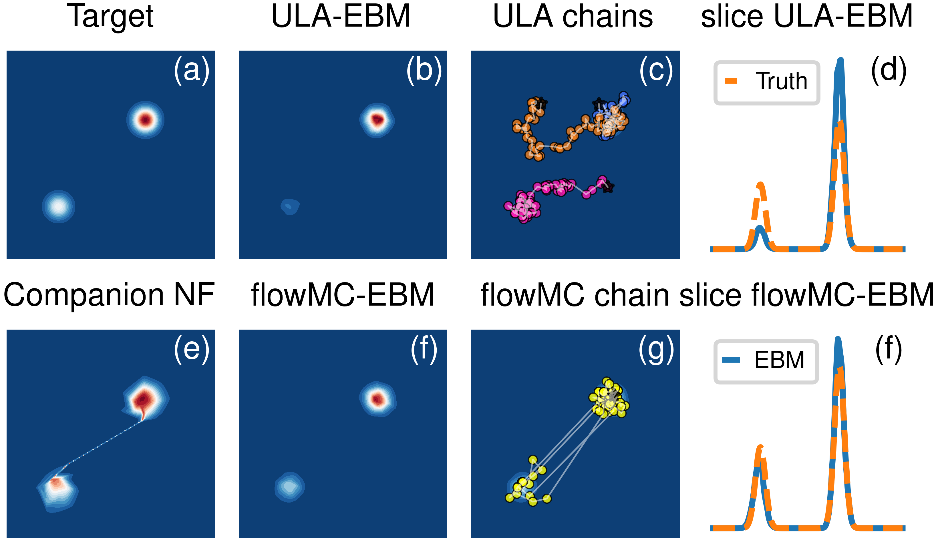
We first illustrate the difficulty of learning relative weights with persistent ULA-EBM training on a 2D mixture of Gaussians (Figure 1). The incapacity of ULA to mix between the modes ((c) versus (g)), introduces a biais in the estimation of the gradient (2), which leads to an over-correction of mismatched weights: ULA-EBM entirely entirely erases a mode multiple times during training, before recreating it and the final weight at which the EBM training stops is not a robust estimation of the target weights (Figure 1 Right). In flowMC-EBM training on the other hand, calibrated negative samples lead to a stable estimation of the weights during learning and a final accurate density estimation ((f) and (h)). The companion flow (e), more constrained in its parametrization, does not achieve a fit as accurate as the EBM, yet its match with the EBM remains good enough to facilitate the fast-mixing MCMC key to success. A detailed comparison including more algorithms from Related Works is also presented in Section C.3.

Table 1: Median squared error on log-density (

\underset{x}{\operatorname{med}}(\log\rho_{\theta}(x)-\log\rho^{\star}(x))^{2})

. Best metrics in bold.

	8 Gaussians	Rings
ULA-EBM	1.86	5.39
NT-EBM	0.97	0.62
CoopFlow	58.75	7.78
flowMC-EBM	0.94	0.40

2D distributions with more modes and complicated geometries.

We benchmark approaches combining EBMs and NFs on the 2D distributions 8-Gaussians and rings. The different models shared the same EBM/flow architecture and were trained for the same number of iterations. The final densities displayed in Figure 2 highlight that our algorithm outperforms competitors in weighting the different modes. This is quantitatively confirmed by the energy errors computed in Table 1. See Section C.4 for more details.

High dimensional mixture

Table 2: Maximum

\hat{R}

across dimension of negative samples on Gaussian mixture computed on 128 independent chains started from the persistent state (or from the flow for CoopFlow). Figure 6 in Section C.5 )

	Dim. 16	Dim. 32	Dim. 64
CoopFlow	20.52	44.12	51.66
NT-EBM	2.02	2.50	3.10
ULA-EBM	7.30	9.29	90.90
flowMC-EBM	1.01	1.01	1.05

We now consider an equally-weighted mixture of 4 Gaussians in dimensions 16, 32 and 64. We compare here again flowMC-EBM with NT-EBM and CoopFlow, yet focusing this time on characterizing the mixing of the chains throughout learning. Using identical EBM/flow architectures trained for the same number of iterations, we report the $\hat{R}$ metric of the negative chains for each model at the end of training in Table 2 for the end of training and in Section C.5 throughout training. Meant to compare the intra-chain variance and the inter-chains variance, reaching a $\hat{R}$ close to 1 is a necessary criteria of convergence of an MCMC (Vehtari et al. 2021). flowMC-EBM is the only algorithm allowing proper mixing. See Section C.5 for more details.

CIFAR 10

Given our computational budget, we were able to train a flowMC-EBM producing samples of medium quality (see Figure 8 of Section C.6 along with training details). Nonetheless, negative chains mix between modes as the companion NF proposal’s are accepted around 5-10% of the time. Given the number of parameters reported in related work, we expect that a more expressive flow and energy parametrization would improve the outcome.

5 Conclusion

By combining an EBM and NF, we manage to tackle the generative models trilemma described in (Xiao et al. 2022). The trilemma states that among the desirable properties of (i) fast sampling, (ii) high-quality samples and (iii) mode-coverage/diversity of the produced samples, a generative model typically only features two out of three. Our numerical experiments show that the cost of training two models is compensated by obtaining a strategy without compromises with respect to the three aspects. Going even further than mode-coverage, we show that our algorithm enables a precise evaluation of the mode relative weights, a topic rarely discussed in the literature.

Acknowledgements

M.G. thanks Eric Vanden-Eijnden for insightful discussions. L.G. and M.G. acknowledge funding from Hi! Paris. The work was partly supported by ANR-19-CHIA-0002-01 “SCAI”. Part of this research has been carried out under the auspice of the Lagrange Center for Mathematics and Computing.

References

Albergo et al. (2019) Albergo, M., Kanwar, G., and Shanahan, P. Flow-based generative models for Markov chain Monte Carlo in lattice field theory. Physical Review D, 100(3):034515, August 2019. ISSN 2470-0010, 2470-0029. doi: 10.1103/PhysRevD.100.034515. URL https://link.aps.org/doi/10.1103/PhysRevD.100.034515.
An et al. (2021) An, D., Xie, J., and Li, P. Learning deep latent variable models by short-run mcmc inference with optimal transport correction. In Proceedings of the IEEE/CVF Conference on Computer Vision and Pattern Recognition (CVPR), pp. 15415–15424, June 2021.
Arbel et al. (2021) Arbel, M., Zhou, L., and Gretton, A. Generalized energy based models. In International Conference on Learning Representations, 2021. URL https://openreview.net/forum?id=0PtUPB9z6qK.
Béreux et al. (2023) Béreux, N., Decelle, A., Furtlehner, C., and Seoane, B. Learning a restricted Boltzmann machine using biased Monte Carlo sampling. SciPost Physics, 14(3):032, March 2023. ISSN 2542-4653. doi: 10.21468/SciPostPhys.14.3.032. URL https://scipost.org/10.21468/SciPostPhys.14.3.032.
Cornish et al. (2020) Cornish, R., Caterini, A., Deligiannidis, G., and Doucet, A. Relaxing Bijectivity Constraints with Continuously Indexed Normalising Flows. Proceedings of the 37 th International Conference on Machine Learning, PMLR 119, 2020.
Dai et al. (2019) Dai, B., Liu, Z., Dai, H., He, N., Gretton, A., Song, L., and Schuurmans, D. Exponential Family Estimation via Adversarial Dynamics Embedding. In Wallach, H., Larochelle, H., Beygelzimer, A., Alché-Buc, F. d., Fox, E., and Garnett, R. (eds.), Advances in Neural Information Processing Systems, volume 32. Curran Associates, Inc., 2019. URL https://proceedings.neurips.cc/paper_files/paper/2019/file/767d01b4bac1a1e8824c9b9f7cc79a04-Paper.pdf.
Dinh et al. (2017) Dinh, L., Sohl-Dickstein, J., and Bengio, S. Density estimation using real NVP. In International Conference on Learning Representations, 2017. URL https://openreview.net/forum?id=HkpbnH9lx.
Du & Mordatch (2019) Du, Y. and Mordatch, I. Implicit Generation and Modeling with Energy Based Models. In Advances in Neural Information Processing Systems, volume 32. Curran Associates, Inc., 2019. URL https://papers.nips.cc/paper_files/paper/2019/hash/378a063b8fdb1db941e34f4bde584c7d-Abstract.html.
Gabrie et al. (2022) Gabrie, M., Rotskoff, G. M., and Vanden-Eijnden, E. Adaptive monte carlo augmented with normalizing flows. Proceedings of the National Academy of Sciences, 119(10):e2109420119, 2022. doi: 10.1073/pnas.2109420119. URL https://www.pnas.org/doi/abs/10.1073/pnas.2109420119.
Gabrié et al. (2015) Gabrié, M., Tramel, E. W., and Krzakala, F. Training Restricted Boltzmann Machines via the Thouless-Anderson-Palmer Free Energy. Advances in Neural Information Processing Systems 28, pp. 640–648, June 2015. ISSN 1063-6919. doi: 10.1109/CVPRW.2009.5206577. URL http://arxiv.org/abs/1506.02914. arXiv: 1506.02914 Publisher: IEEE ISBN: 9781424439935.
Grathwohl et al. (2020) Grathwohl, W., Wang, K.-C., Jacobsen, J.-H., Duvenaud, D., and Zemel, R. Learning the stein discrepancy for training and evaluating energy-based models without sampling. In III, H. D. and Singh, A. (eds.), Proceedings of the 37th International Conference on Machine Learning, volume 119 of Proceedings of Machine Learning Research, pp. 3732–3747. PMLR, 13–18 Jul 2020. URL https://proceedings.mlr.press/v119/grathwohl20a.html.
Grathwohl et al. (2021) Grathwohl, W. S., Kelly, J. J., Hashemi, M., Norouzi, M., Swersky, K., and Duvenaud, D. No {mcmc} for me: Amortized sampling for fast and stable training of energy-based models. In International Conference on Learning Representations, 2021. URL https://openreview.net/forum?id=ixpSxO9flk3.
Grenioux et al. (2023) Grenioux, L., Durmus, A., Moulines, E., and Gabrie, M. On sampling with approximate transport maps. arXiv preprint 2302.04763, 2023. doi: 10.48550/ARXIV.2302.04763. URL https://arxiv.org/abs/2302.04763.
Gutmann & Hyvärinen (2010) Gutmann, M. and Hyvärinen, A. Noise-contrastive estimation: A new estimation principle for unnormalized statistical models. In Teh, Y. W. and Titterington, M. (eds.), Proceedings of the Thirteenth International Conference on Artificial Intelligence and Statistics, volume 9 of Proceedings of Machine Learning Research, pp. 297–304, Chia Laguna Resort, Sardinia, Italy, 13–15 May 2010. PMLR. URL https://proceedings.mlr.press/v9/gutmann10a.html.
Hackett et al. (2021) Hackett, D. C., Hsieh, C.-C., Albergo, M. S., Boyda, D., Chen, J.-W., Chen, K.-F., Cranmer, K., Kanwar, G., and Shanahan, P. E. Flow-based sampling for multimodal distributions in lattice field theory, July 2021. URL http://arxiv.org/abs/2107.00734. arXiv:2107.00734 [cond-mat, physics:hep-lat].
Hinton (2002) Hinton, G. E. Training products of experts by minimizing Contrastive divergence. Neural computation, 14:1771–1800, 2002.
Hinton (2012) Hinton, G. E. A practical guide to training restricted boltzmann machines. Neural Networks: Tricks of the Trade: Second Edition, pp. 599–619, 2012.
Hoffman et al. (2019) Hoffman, M. D., Sountsov, P., Dillon, J. V., Langmore, I., Tran, D., and Vasudevan, S. NeuTra-lizing Bad Geometry in Hamiltonian Monte Carlo Using Neural Transport. In 1st Symposium on Advances in Approximate Bayesian Inference, 2018 1–5, 2019. URL http://arxiv.org/abs/1903.03704.
Hyvärinen (2005) Hyvärinen, A. Estimation of Non-Normalized Statistical Models by Score Matching. Journal of Machine Learning Research, 6(24):695–709, 2005. URL http://jmlr.org/papers/v6/hyvarinen05a.html.
Jerfel et al. (2021) Jerfel, G., Wang, S., Wong-Fannjiang, C., Heller, K. A., Ma, Y., and Jordan, M. I. Variational refinement for importance sampling using the forward kullback-leibler divergence. In Uncertainty in Artificial Intelligence, pp. 1819–1829. PMLR, 2021.
Kobyzev et al. (2021) Kobyzev, I., Prince, S. J., and Brubaker, M. A. Normalizing flows: An introduction and review of current methods. IEEE Transactions on Pattern Analysis and Machine Intelligence, 43(11):3964–3979, 2021. doi: 10.1109/TPAMI.2020.2992934.
McNaughton et al. (2020) McNaughton, B., Milošević, M. V., Perali, A., and Pilati, S. Boosting Monte Carlo simulations of spin glasses using autoregressive neural networks. Physical Review E, 101(5):053312, May 2020. ISSN 2470-0045, 2470-0053. doi: 10.1103/PhysRevE.101.053312. URL http://arxiv.org/abs/2002.04292. arXiv:2002.04292 [cond-mat, physics:physics].
Müller et al. (2019) Müller, T., Mcwilliams, B., Rousselle, F., Gross, M., and Novák, J. Neural Importance Sampling. ACM Transactions on Graphics, 38(5):1–19, October 2019. ISSN 0730-0301, 1557-7368. doi: 10.1145/3341156. URL https://dl.acm.org/doi/10.1145/3341156.
Naesseth et al. (2021) Naesseth, C. A., Lindsten, F., and Blei, D. Markovian Score Climbing: Variational Inference with KL(p||q), February 2021. URL http://arxiv.org/abs/2003.10374. arXiv:2003.10374 [cs, stat].
Nicoli et al. (2020) Nicoli, K. A., Nakajima, S., Strodthoff, N., Samek, W., M üller, K.-R., and Kessel, P. Asymptotically unbiased estimation of physical observables with neural samplers. Physical Review E, 101(2):023304, February 2020. ISSN 2470-0045, 2470-0053. doi: 10.1103/PhysRevE.101.023304. URL http://arxiv.org/abs/1910.13496. arXiv:1910.13496 [cond-mat, stat].
Nijkamp et al. (2019) Nijkamp, E., Hill, M., Zhu, S.-C., and Wu, Y. N. Learning non-convergent non-persistent short-run mcmc toward energy-based model. In Wallach, H., Larochelle, H., Beygelzimer, A., d'Alché-Buc, F., Fox, E., and Garnett, R. (eds.), Advances in Neural Information Processing Systems, volume 32. Curran Associates, Inc., 2019. URL https://proceedings.neurips.cc/paper_files/paper/2019/file/2bc8ae25856bc2a6a1333d1331a3b7a6-Paper.pdf.
Nijkamp et al. (2020a) Nijkamp, E., Hill, M., Han, T., Zhu, S.-C., and Wu, Y. N. On the anatomy of mcmc-based maximum likelihood learning of energy-based models. Proceedings of the AAAI Conference on Artificial Intelligence, 34(04):5272–5280, Apr. 2020a. doi: 10.1609/aaai.v34i04.5973. URL https://ojs.aaai.org/index.php/AAAI/article/view/5973.
Nijkamp et al. (2020b) Nijkamp, E., Pang, B., Han, T., Zhou, L., Zhu, S.-C., and Wu, Y. N. Learning multi-layer latent variable model via variational optimization of short run mcmc for approximate inference. In Vedaldi, A., Bischof, H., Brox, T., and Frahm, J.-M. (eds.), Computer Vision – ECCV 2020, pp. 361–378, Cham, 2020b. Springer International Publishing. ISBN 978-3-030-58539-6.
Nijkamp et al. (2022) Nijkamp, E., Gao, R., Sountsov, P., Vasudevan, S., Pang, B., Zhu, S.-C., and Wu, Y. N. MCMC should mix: Learning energy-based model with neural transport latent space MCMC. In International Conference on Learning Representations, 2022. URL https://openreview.net/forum?id=4C93Qvn-tz.
Noé et al. (2019) Noé, F., Olsson, S., Köhler, J., and Wu, H. Boltzmann generators: Sampling equilibrium states of many-body systems with deep learning. Science, 365(6457):eaaw1147, September 2019. ISSN 0036-8075, 1095-9203. doi: 10.1126/science.aaw1147. URL https://www.science.org/doi/10.1126/science.aaw1147.
Papamakarios et al. (2021) Papamakarios, G., Nalisnick, E., Rezende, D. J., Mohamed, S., and Lakshminarayanan, B. Normalizing flows for probabilistic modeling and inference. Journal of Machine Learning Research, 22(57):1–64, 2021. URL http://jmlr.org/papers/v22/19-1028.html.
Parno & Marzouk (2018) Parno, M. D. and Marzouk, Y. M. Transport Map Accelerated Markov Chain Monte Carlo. SIAM/ASA Journal on Uncertainty Quantification, 6(2):645–682, January 2018. ISSN 2166-2525. doi: 10.1137/17M1134640. URL https://epubs.siam.org/doi/10.1137/17M1134640.
Rezende & Mohamed (2015) Rezende, D. and Mohamed, S. Variational Inference with Normalizing Flows. In Proceedings of the 32nd International Conference on Machine Learning, pp. 1530–1538. PMLR, June 2015. URL https://proceedings.mlr.press/v37/rezende15.html. ISSN: 1938-7228.
Roberts & Tweedie (1996) Roberts, G. O. and Tweedie, R. L. Exponential convergence of langevin distributions and their discrete approximations. Bernoulli, 2(4):341–363, 1996. ISSN 13507265. URL http://www.jstor.org/stable/3318418.
Rubin (1987) Rubin, D. B. The calculation of posterior distributions by data augmentation: Comment: A noniterative sampling/importance resampling alternative to the data augmentation algorithm for creating a few imputations when fractions of missing information are modest: The sir algorithm. Journal of the American Statistical Association, 82(398):543–546, 1987. ISSN 01621459. URL http://www.jstor.org/stable/2289460.
Salmona et al. (2022) Salmona, A., De Bortoli, V., Delon, J., and Desolneux, A. Can Push-forward Generative Models Fit Multimodal Distributions? In Koyejo, S., Mohamed, S., Agarwal, A., Belgrave, D., Cho, K., and Oh, A. (eds.), Advances in Neural Information Processing Systems, volume 35, pp. 10766–10779. Curran Associates, Inc., 2022. URL https://proceedings.neurips.cc/paper_files/paper/2022/file/45f0d179ef7e10eb7366550cd4e574ae-Paper-Conference.pdf.
Samsonov et al. (2022) Samsonov, S., Lagutin, E., Gabrié, M., Durmus, A., Naumov, A., and Moulines, E. Local-global mcmc kernels: the best of both worlds. In Advances in Neural Information Processing Systems, 2022.
Song & Ermon (2019) Song, Y. and Ermon, S. Generative Modeling by Estimating Gradients of the Data Distribution. In Wallach, H., Larochelle, H., Beygelzimer, A., Alché-Buc, F. d., Fox, E., and Garnett, R. (eds.), Advances in Neural Information Processing Systems, volume 32. Curran Associates, Inc., 2019. URL https://proceedings.neurips.cc/paper_files/paper/2019/file/3001ef257407d5a371a96dcd947c7d93-Paper.pdf.
Song & Kingma (2021) Song, Y. and Kingma, D. P. How to train your energy-based models, 2021.
Tieleman (2008) Tieleman, T. Training restricted Boltzmann machines using approximations to the likelihood gradient. In Proceedings of the 25th international conference on Machine learning - ICML ’08, pp. 1064–1071, Helsinki, Finland, 2008. ACM Press. ISBN 978-1-60558-205-4. doi: 10.1145/1390156.1390290. URL http://portal.acm.org/citation.cfm?doid=1390156.1390290.
Vehtari et al. (2021) Vehtari, A., Gelman, A., Simpson, D., Carpenter, B., and Bürkner, P.-C. Rank-Normalization, Folding, and Localization: An Improved $\widehat{R}$ for Assessing Convergence of MCMC (with Discussion). Bayesian Analysis, 16(2):667 – 718, 2021. doi: 10.1214/20-BA1221. URL https://doi.org/10.1214/20-BA1221.
Welling & Hinton (2002) Welling, M. and Hinton, G. E. A New Learning Algorithm for Mean Field Boltzmann Machines. In Dorronsoro, J. R. (ed.), Artificial Neural Networks — ICANN 2002, pp. 351–357, Berlin, Heidelberg, 2002. Springer Berlin Heidelberg. ISBN 978-3-540-46084-8.
Wu et al. (2019) Wu, D., Wang, L., and Zhang, P. Solving Statistical Mechanics Using Variational Autoregressive Networks. Physical Review Letters, 122(8):080602, February 2019. ISSN 0031-9007, 1079-7114. doi: 10.1103/PhysRevLett.122.080602. URL http://arxiv.org/abs/1809.10606. arXiv:1809.10606 [cond-mat, stat].
Xiao et al. (2020) Xiao, Z., Yan, Q., and Amit, Y. Exponential tilting of generative models: Improving sample quality by training and sampling from latent energy, 2020.
Xiao et al. (2021) Xiao, Z., Kreis, K., Kautz, J., and Vahdat, A. Vaebm: A symbiosis between variational autoencoders and energy-based models. In International Conference on Learning Representations, 2021. URL https://openreview.net/forum?id=5m3SEczOV8L.
Xiao et al. (2022) Xiao, Z., Kreis, K., and Vahdat, A. Tackling the generative learning trilemma with denoising diffusion GANs. In International Conference on Learning Representations, 2022. URL https://openreview.net/forum?id=JprM0p-q0Co.
Xie et al. (2018) Xie, J., Lu, Y., Gao, R., and Wu, Y. N. Cooperative learning of energy-based model and latent variable model via mcmc teaching. Proceedings of the AAAI Conference on Artificial Intelligence, 32(1), Apr. 2018. doi: 10.1609/aaai.v32i1.11834. URL https://ojs.aaai.org/index.php/AAAI/article/view/11834.
Xie et al. (2021) Xie, J., Zheng, Z., and Li, P. Learning energy-based model with variational auto-encoder as amortized sampler. Proceedings of the AAAI Conference on Artificial Intelligence, 35(12):10441–10451, May 2021. doi: 10.1609/aaai.v35i12.17250. URL https://ojs.aaai.org/index.php/AAAI/article/view/17250.
Xie et al. (2022) Xie, J., Zhu, Y., Li, J., and Li, P. A tale of two flows: Cooperative learning of langevin flow and normalizing flow toward energy-based model. In International Conference on Learning Representations, 2022. URL https://openreview.net/forum?id=31d5RLCUuXC.

Appendix A Algorithms

We recall useful algorithms: the Unagjusted Langevin (ULA) in Algorithm 2, the persistent ULA-EBM training in Algorithm 3, the Metropolis Adjusted Langevin Algorithm (MALA) in Algorithm 4 and finally the flowMC sampler in Algorithm 5. We also recall the Iterated Sampling Importance Resampling (i-SIR) in Algorithm 6 which can be used as a drop-in replacement of steps 1.a-1.b of the flowMC algorithm (Algorithm 5) as suggested by (Samsonov et al. 2022).

Algorithm 2 Unadjusted Langevin algorithm (ULA) with target distribution

\pi

Input:

x^{(0)}

initial sample,

\eta

step-size,

L

number of MCMC steps

Output:

(x^{(k)})_{k=1}^{L}

samples according to

\pi

while

k<L;k=1

x^{(k)}\sim\mathcal{N}(x^{(k-1)}+\eta\nabla\log\pi(x^{(k-1)}),2\eta I_{d})

end while

Algorithm 3 ULA-EBM training step with persistent initialization (Du & Mordatch 2019; Nijkamp et al. 2020a)

Input: Data distribution

p^{\star}

, EBM parameter

\theta_{k}

, learning rate

\gamma

, batch size

n

, ULA step size

\eta

, number of ULA steps

L

, persistent state

\{\tilde{x}_{i}\}_{i=1}^{n}

Output: New EBM parameter

\theta_{k+1}

1. Draw positive samples

\{x^{(+)}_{i}\}_{i=1}^{n}\sim p^{\star}

2. Draw negative samples

x^{(-)}_{i}=\mathrm{ULA}(-E_{\theta_{k}},\tilde{x}_{i},\eta,L)\text{ for }i=1\dots n\;

3. Update persistent state

\{\tilde{x}_{i}\}_{i=1}^{n}=\{x^{(-)}_{i}\}_{i=1}^{n}

4. Perform a GD step on

-\ell_{\rm EBM}(\theta)

(cf Equation 2)

Algorithm 4 Metropolis-adjusted Langevin algorithm (MALA) with target distribution

\pi

Input:

x^{(0)}

initial sample,

\eta

step-size,

L

number of MCMC steps

Output:

(x^{(k)})_{k=1}^{L}

samples according to

\pi

while

k<L;k=1

1. Sample the local proposal

x^{(k)}\sim\mathcal{N}(x^{(k-1)}+\eta\nabla\log\pi(x^{(k-1)}),2\eta I_{d})

2. Metropolis-Hastings accept-reject

x^{(k)}=x^{(k-1)}\text{ with prob. }

1-\min\left[1,\frac{\pi(x^{(k)})q(x^{(k-1)}|x^{(k)})}{\pi(x^{(k-1)})q(x^{(k)}|x^{(k-1)})}\right]

where

q(x^{\prime}|x)=\exp(-\left\lVert x^{\prime}-x-\eta\nabla\log\pi(x)\right\rVert^{2}/(4\eta))

end while

Algorithm 5 FlowMC adaptive sampling of target distribution

\pi

(Gabrie et al. 2022)

Input:

x^{(0)}

initial sample,

T_{\alpha}

initial flow,

\rho

base distribution,

\eta

MALA step-size,

\gamma

flow learning rate,

n_{\rm MALA}

number of MALA steps,

L

number of MCMC steps

Output:

(x^{(k)})_{k=1}^{L}

samples according to

\pi

while

k<N;k=1

1.a Sample the flow

x^{(k)}\sim\lambda_{T_{\alpha}}^{\rho}(x)

1.b Metropolis-Hastings accept-reject

x^{(k)}=x^{(k-1)}\text{ with prob. }

1-\min\left[1,\frac{\pi(x^{(k)})\lambda_{T_{\alpha}}^{\rho}(x^{(k-1)})}{\pi(x^{(k-1)})\lambda_{T_{\alpha}}^{\rho}(x^{(k)})}\right]

2. Sample with MALA from

x^{(k)}

x^{(k+1:k+n_{\rm MALA}+1)}=\mathrm{MALA}(\log\pi,x^{(k)},\eta,n_{\rm MALA})

k=k+1+n_{\rm MALA}

3. Likelihood ascent step on the flow

\alpha=\alpha+\gamma\sum_{k^{\prime}<k}\ln\lambda_{T_{\alpha}}^{\rho}(x^{(k^{\prime})})

end while

Algorithm 6 Iterated Sampling Importance Resampling (i-SIR) (Rubin 1987)

Input:

x^{(0)}

initial sample,

\lambda

proposal distribution,

N

number of particles,

L

number of MCMC steps

Output:

(x^{(k)})_{k=1}^{L}

samples according to

\pi

while

k<L;k=1

1. Draw a pool of proposals

y_{2:N}^{(k+1)}\sim\lambda

2. Set the

x^{(k)}

as the first element of the pool

y_{1}^{(k+1}=x^{(k)}

3. Compute the importance weights

w_{i}^{(k+1)}=w(y_{i}^{(k+1)})/\sum_{j=1}^{N}w(y_{j}^{(k+1)})

for all

i=1,\ldots,N

where

w=\pi/\lambda

4. Select the next state

i^{(k+1)}\sim\mathcal{M}(w_{1}^{(k+1)},\ldots,w_{N}^{(k+1)})

5. Update the next state

x^{(k+1)}=y_{i^{(k+1)}}^{(k+1)}

end while

Appendix B Gradients of tilted distribution

This section provides the proof of the remark at the beginning of Section 3. Let’s consider a tilted EBM as in Equation 6 with $E_{\theta}:\mathbb{R}^{d}\to\mathbb{R}$ a parametrized energy function, $Z_{\theta}$ the associated normalizing constant of $p_{\theta}^{\rho}$ and $\rho$ the base distribution. We have that $\nabla_{\theta}\log p_{\theta}^{\rho}(x)=-\nabla_{\theta}E_{\theta}(x)-\nabla_{\theta}\log Z_{\theta}$ . The second term can be expressed as an expectation over $p_{\theta}^{\rho}$

	$\displaystyle\nabla_{\theta}\log Z_{\theta}$	$\displaystyle=\nabla_{\theta}\log\int\exp(-E_{\theta}(x))\rho(x)\mathrm{d}x$
		$\displaystyle=\left(\int\exp(-E_{\theta}(x))\rho(x)\mathrm{d}x\right)^{-1}\nabla_{\theta}\int\exp(-E_{\theta}(x))\rho(x)\mathrm{d}x$
		$\displaystyle=\left(\int\exp(-E_{\theta}(x))\rho(x)\mathrm{d}x\right)^{-1}\int\nabla_{\theta}\exp(-E_{\theta}(x))\rho(x)\mathrm{d}x$
		$\displaystyle=\left(\int\exp(-E_{\theta}(x))\rho(x)\mathrm{d}x\right)^{-1}\int\exp(-E_{\theta}(x))(-\nabla_{\theta}E_{\theta}(x))\rho(x)\mathrm{d}x$
		$\displaystyle=\int\left(\int\exp(-E_{\theta}(y))\rho(y)\mathrm{d}y\right)^{-1}\exp(-E_{\theta}(x))(-\nabla_{\theta}E_{\theta}(x))\rho(x)\mathrm{d}x$
		$\displaystyle=\int(-\nabla_{\theta}E_{\theta}(x))p_{\theta}^{\rho}(x)\mathrm{d}x$
		$\displaystyle=\mathbb{E}_{p_{\theta}^{\rho}}[-\nabla_{\theta}E_{\theta}(X)]\,.$

The gradient of the maximum likelihood objective can then be formulated as

	$\displaystyle\nabla_{\theta}\ell_{\rm EBM}(\theta)$	$\displaystyle=\mathbb{E}_{p^{\star}}[\nabla_{\theta}\log p_{\theta}(X)]$
		$\displaystyle=\mathbb{E}_{p^{\star}}[-\nabla_{\theta}E_{\theta}(X)-\nabla_{\theta}\log Z_{\theta}]$
		$\displaystyle=-\mathbb{E}_{p^{\star}}[\nabla_{\theta}E_{\theta}(X)]+\mathbb{E}_{p_{\theta}^{\rho}}[\nabla_{\theta}E_{\theta}(X)]\,.$

Appendix C Experiments

C.1 Common remarks on implementation of the different EBM training algorithms throughout the numerics

While Hamiltonian Monte Carlo (HMC) can be used instead of Langevin as a local MCMC sampler (Nijkamp et al. 2022), we stick to MALA in our implementations of CoopFlow, NT-EBM and flowMC-EBM for two reasons : (i) it is much faster than HMC ²² 2 Only one gradient per generated sample. (ii) it makes the comparison between models easier. Moreover, most of the EBM training algorithms in the literature originally used only a few MCMC steps at each iteration. In our benchmark of these algorithms, we typically use more MCMC steps. Finally, we used specific version of CoopFlow and ULA-EBM algorithms.

Coop Flow

For CoopFlow (Xie et al. 2022) we used the ”best” version of their algorithm where the flow is pre-trained on samples from $p^{\star}$ . During the coupled training of the EBM, the pre-trained flow will be initially frozen for less than 5% of the total training time. We also disabled the noise in Langevin steps as advised by the authors.

ULA-EBM

For the ULA-EBM, the hyper-parameters (custom temperature and learning rate) were selected using the recommendations from (Nijkamp et al. 2020a).

FlowMC with i-SIR updates

In practice, we use the flowMC algorithm (Algorithm 5) with the i-SIR algorithm (Algorithm 6) as a global sampler (i.e. for steps 1.a to 1.b of the flowMC algorithm). As it accepts one flow proposal from a large pool of samples, this algorithm enables shorter decorelation times provided enough memory and parallel computation capabilities.

C.2 Motivating example

The first example from Section 4 uses an unequilibrated mixture of two multivariate normal distributions in 2D

p^{\star}(x)=\frac{1}{3}\mathcal{N}(-1.5\mathbf{1}_{2},0.05I_{2})+\frac{2}{3}\mathcal{N}(+1.5\mathbf{1}_{2},0.1I_{2})\,

where $\mathbf{1}_{d}$ is the vector with only unit coordinates in dimension $d$ . Both models were trained for 75 epochs on a dataset of length 16384 using a persistent state of size 1024 and a batch size of 64 with a learning rate of 0.01 (same one for the flow and the EBM). The global steps are i-SIR steps with 32 particles. The Langevin samplers used a step size of 0.01. The classic EBM used 10 MCMC steps at each step and the flowMC-EBM used the same number of steps decomposed with 2 global steps between two sequence of 4 local steps. We used the same parameterization for the EBM as in (Nijkamp et al. 2020a) (about 10k parameters). The flow is a RealNVP (Dinh et al. 2017) with 4 layers each one featuring MLPs with 16 neurons on 3 layers (about 1k parameters total).

C.3 Extended motivating example

This additional motivating example aims at building intuition on why other methods are failing at relative weights estimation. This experiment uses an 2D unequilibrated mixture of four Gaussians $p^{\star}=\sum_{i=1}^{4}w_{i}\mathcal{N}(\mu_{i},0.05I_{2})$ where the $\mu_{i}$ are evenly distributed on a horizontal axis between $x=-3$ and $x=3$ and $w=(0.1,0.2,0.3,0.4)$ .

[Uncaptioned image] — Figure 3: Estimated energies using different algorithms on the extended motivating example.

Algorithm	MSE of the init. wrt $E_{\theta}$	MSE of the neg. samples wrt $E_{\theta}$	MSE of $E_{\theta}$ wrt $-\log p^{\star}$
ULA-EBM	1.19e-03	1.79e-03	1.24e-03
CoopFlow	1.21e-01	1.11e-01	1.24e-01
NT-EBM	9.27e-04	3.85e-04	9.87e-04
flowMC-EBM	5.19e-04	3.12e-05	4.29e-04

The obtained EBMs are presented in Figure 3. Table 3 provides a quantitative comparison between the different algorithms. The mean squared error of samples $X$ with respect to distribution $p$ are computed by partitioning the space in as much regions as the number of modes of $p$ (see Figure 4) and then building an histogram of the samples $X$ depending on which zone each sample is. The error is computed against the weights of the distribution $p$ . For the distribution $E_{\theta}$ , the weights are computed by manually summing the mass in each region corresponding to the modes of $p^{\star}$ .

The second column of Table 3 represents the quality of the initialisation of the negative chains with respect to the current EBM - this is the error that CoopFlow should minimize by using a flow. The third column represents the error of the negative samples with respect to the current EBM - this is the error that NT-EBM should minimize by mixing in the latent space. Table 3 shows that our algorithm is the only one minimizing both errors leading to a better EBM (see the fourth column). Our algorithm improves the initialization by using calibrated MCMC algorithms and improves negative samples by using the companion normalizing flow to visit even more modes during the sampling phase.

The failure of CoopFlow at providing good initialization is likely due to the fact that pre-training the flow on data provide bad starting samples if the current EBM’s weights are not close to the data weights : at the end of training, the weights of its flow are $(0.11,0.20,0.29,0.40)$ which is very accurate with respect to data but the MSE with respect to the EBM is of order $10^{-1}$ . This is worsen by the lack of any MCMC calibration on the initialisation and the negative samples. The failure of NT-EBM at improving its initialization error is likely due to the fact that the local sampler isn’t mixing in the latent space (as suggested by (Grenioux et al. 2023)) as shown in Figure 5.

The hyper-parameters of each algorithm are summarized in Table 5. The Use only last step ? column correspond to whether the negative samples are the last elements of the MCMC chains or not. The learning rates is $10^{-2}$ for EBM and NT-EBM and $10^{-3}$ for CoopFlow and our algorithm (flow and EBM). The dataset is 60000 samples large with a batch size of 256 and a persistent size of 8192. The training lasted 100 epochs for each algorithm. The EBM and the flow are the same is in Section C.2. When required, the flows were pretrained for 1024 steps at a $10^{-2}$ learning rate with the reverse KL objective. The global sampler is i-SIR with 64 particles.

Table 4: EBM hyper-parameters for the extended motivating example

Algorithm	MCMC Sampler	# MCMC steps	Use only last step ?	Starting strategy
ULA-EBM	ula with $(1.25\times 10^{-1})^{2}/2$ step size	$512$	yes	uniform
NT-EBM	mala with target acceptance $75\%$	$128$	yes	flow
CoopFlow	ula with $5\times 10^{-4}$ step size	$256$	yes	flow
flowMC-EBM	flowMC with 1 global step and 24 mala local steps	$128$	no	flow

C.4 2D distributions with more modes and complicated geometries.

The 8 Gaussians distribution is a mixture of 8 equally weighted Gaussians $\mathcal{N}(\mu_{i},0.15^{2}I_{2})$ where $\mu_{i}=(\cos(2\pi t_{i}),\sin(2\pi t_{i}))$ and $t_{i}=i/8$ with $i\in\{0,\ldots,7\}$ . The rings distributions is the inverse polar reparametrization of a distribution $p_{z}$ which has itself a decomposition into two univariate marginals $p_{r}$ and $p_{\theta}$ . $p_{r}$ is a mixture of 4 Gaussians $\mathcal{N}(i+1,0.15^{2})$ with $i\in\{0,\ldots,3\}$ describing the radial position and $p_{\theta}$ is a uniform distribution over $[0,2\pi]$ which describe the angular position of the samples.

The hyper-parameters of each algorithm are summarized in Table 5. The Use only last step ? column correspond to whether the negative samples are the last elements of the MCMC chain or not. If subsampling by k is mentioned in the this column, it means that we divided the number of parallel MCMC chains by $k$ and subsampled the resulting chains evenly $k$ times. The learning rates was $10^{-2}$ for EBM and NT-EBM and $10^{-3}$ for CoopFlow and our algorithm (flow and EBM). The dataset was 60000 samples large with a batch size of 256 and a persistent size of 8192. The training lasted 100 epochs for each algorithm. The EBM and the flow are the same is in Section C.2. When required, the flows were pretrained for 1024 steps at a $10^{-2}$ learning rate with the reverse KL objective. The global sampler is i-SIR with 64 particles.

Table 5: EBM hyper-parameters for 8 Gaussians / Rings experiments

Algorithm	MCMC Sampler	# MCMC steps	Use only last step ?	Starting strategy
ULA-EBM	ula with $(1.25\times 10^{-1})^{2}/2$ step size	$512$	yes	uniform
NT-EBM	mala with target acceptance $75\%$	$128$	yes	flow
CoopFlow	ula with $5\times 10^{-4}$ step size	$256$	yes	flow
flowMC-EBM	flowMC with 1 global step and 127 mala local steps	$128$	subsampling by 4	flow

C.5 High-dimensional example

Figure 6: Extended version of figure Table 2 where the

\hat{R}

is displaying along training time

In this experiment, $p^{\star}$ is a mixture of 4 equally weighted isotropic Gaussians $p^{\star}_{i}=\mathcal{N}(\mu_{i},I_{d})$ where the $\mu_{i}$ are defined as $\mu_{1}=a\times(1,1,1,\ldots,1,1,1)$ , $\mu_{2}=a\times(-1,-1,-1,\ldots,1,1,1)$ , $\mu_{2}=-\mu_{2}$ and $\mu_{4}=-\mu_{1}$ and $a=0.5919$ . This specific value of $a$ guarantees that if $X\sim p^{\star}_{i}$ then $\forall j\neq i,\mathbb{P}(\|X-\mu_{j}\|<\|X-\mu_{i}\|)\leq 10^{-10}$ for any dimension $d$ .

The hyper-parameters of each algorithm are summarized in Table 7. The Use only last step ? column correspond to whether the negative samples are the last elements of the MCMC chains or not. If stacked is mentionned in the # MCMC steps column, it means that the $k_{g}$ global steps and $k_{l}$ local steps are considered as a single MCMC step. The learning rates was $10^{-2}$ for EBM and NT-EBM and $10^{-3}$ for CoopFlow and our algorithm (flow and EBM). The dataset was 50000 samples large with a batch size of 128 and a persistent size of 8192. The training lasted 150 epochs for each algorithm. The EBM parametrization is the same as the one described in (Nijkamp et al. 2020a). The global sampler is i-SIR with 128 particles. The flows used here are RealNVPs. The base of the flow is $\rho=\mathcal{N}(0,\sigma^{2}I_{d})$ where $\sigma^{2}$ is the maximum variance of $\pi$ along each dimension. All the coupling layers have 3 hidden layers initialized with very small weights $(\simeq 10^{-6})$ . The other hyper-parameters can be found in table Table 6. When required, the flows were pretrained for 512 steps at a $10^{-2}$ learning rate with the reverse KL objective.

Table 6: RealNVP architecture for the high-dimensional Gaussian mixture

Dimension	Size of hidden layers	# RealNVP blocks
16	32	2
32	39	2
64	51	2

Table 7: EBM hyper-parameters for the high-dimensional mixture experiment

Algorithm	MCMC Sampler	# MCMC steps	Use only last step ?	Starting strategy
ULA-EBM	ula with $10^{-3}$ step size	$512$	yes	gaussian
NT-EBM	mala with target acceptance $75\%$	$128$	yes	flow
CoopFlow	ula with $10^{-4}$ step size	$256$	yes	flow
flowMC-EBM	flowMC with 1 global step and 8 mala local steps	$16$ (stacked)	no	flow

C.6 Image distribution

Figure 7: Energy histograms of our algorithm trained on CIFAR10

We tested our algorithm on the CIFAR10 dataset (see training details below). Given our computational budget, the resulting generative model can produce samples of medium quality (see Figure 8). The global sampler proposals are getting accepted 5-10% of the time. Given number of parameters reported in related work, we expect that a more expressive flow and energy parametrization would improve the outcome. Following the experiments of (Dai et al. 2019), we compute the energy distribution of the generated samples and compare it against the data samples (see Figure 7). The EBM produces sample in the right energy range but not as diverse as the training data.

The flowMC-EBM was trained on the CIFAR10 dataset using a batch size of 128 and for 70 epochs and a persistent size of 1024. The learning rates of the flow and the EBM was $10^{-4}$ with a decay by $0.99$ every 50 batches. We used an L2 regularization with coefficient $10^{-4}$ on the EBM loss i.e., we added a $\ell_{\text{reg}}$ term where $\ell_{\text{reg}}(\theta,\{x^{(-)}_{i},x^{(+)}_{i}\}_{i=1}^{n})=\lambda\sum_{i=1}^{n}(E_{\theta}(x^{(-)}_{i}))^{2}+(E_{\theta}(x^{(+)}_{i}))^{2}$ with $\lambda=10^{-4}$ . The sampler stacked 1 i-SIR global step with 128 particles and 32 local steps of MALA three times in total to build the negative samples.

The dataset was centered between -1 and 1 and also dequantized (ie. if $x$ is an image with integer pixels in range $[0,255]$ then its dequantization is $\tilde{x}=(255x+U)/256$ where $U\sim\mathcal{U}([0,1])$ ). The dataset was augmented with random horizontal flipping.

The EBM used was the one described in (Du & Mordatch 2019) and used in (Xie et al. 2022) with a smaller last MLP layer (about 4.5M parameters only). The flow is a RealNVP taken from this Github repository with base_dim to 64 and 6 residual blocks (about 4M parameters). The flow was stacked with an affine transformation bringing the images in $[0,1]$ and the logisitic transformation described in (Dinh et al. 2017). The base of the flow is a standard centered multivariate Gaussian $\mathbf{N}(0,I_{3\times 32\times 32})$ and the prior of the EBM (see Equation 6) was pushed through the additional transformations stacked onto the flow.