跳到论文正文
W Papers独立论文阅读器 arXiv:2306.00308 论文正文 计算阅读时间 · 0%
引用这篇论文根据当前论文元数据生成,正式投稿前建议核对。


License: CC BY 4.0
arXiv:2306.00308v1 [cs.PL] 01 Jun 2023

A Formal Model for Secure Multiparty Computations

Amy Rathore Affiliation: Department of Computer Science and Engineering, University at Buffalo    Marina Blanton Affiliation: Department of Computer Science and Engineering, University at Buffalo    Marco Gaboardi Affiliation: Department of Computer Science, Boston University    Lukasz Ziarek Affiliation: Department of Computer Science and Engineering, University at Buffalo
Abstract

Although Secure Multiparty Computation (SMC) has seen considerable development in recent years, its use is challenging, resulting in complex code which obscures whether the security properties or correctness guarantees hold in practice. For this reason, several works have investigated the use of formal methods to provide guarantees for SMC systems. However, these approaches have been applied mostly to domain specific languages (DSL), neglecting general-purpose approaches. In this paper, we consider a formal model for an SMC system for annotated C programs. We choose C due to its popularity in the cryptographic community and being the only general-purpose language for which SMC compilers exist. Our formalization supports all key features of C – including private-conditioned branching statements, mutable arrays (including out of bound array access), pointers to private data, etc. We use this formalization to characterize correctness and security properties of annotated C, with the latter being a form of non-interference on execution traces. We realize our formalism as an implementation in the PICCO SMC compiler and provide evaluation results on SMC programs written in C.

1 Introduction

Secure Multiparty Computation (SMC) allows multiple parties to jointly compute over private data, revealing only the outcomes of the computation to designated recipients. Secure computation is needed in many domains, particularly the medical, military, and financial sectors. SMC is commonly implemented using low-level techniques like secret sharing [37], garbled circuits [41], or homomorphic encryption [12, 29]. These low-level techniques are designed to enable computations among parties which are secure and efficient. While these low-level techniques provide efficiency, their use makes programming SMC applications challenging and error prone. To address this concern, several works have proposed high-level languages, DSLs, or language extensions providing abstractions, which can then be compiled down to low-level SMC primitives, to support programmers in writing SMC applications. As a result, there now exists a plethora of languages providing different expressivity, offering different features and performance trade-offs, using different threat models, and suitable for different domains. Similarly, there exist a number of SMC DSLs. Although DSLs can make it easier to write SMC programs, there remains a disconnect between the DSL and its integration with the language of the underlying implementation of the compiled protocol.

In the effort to unify our knowledge in this space, a recent work [15] compared several compilers and tools in terms of their expressivity and usability. We highlight two items among the lessons learned and recommendations to the community. First, there were numerous correctness issues and undocumented limitations present in the works surveyed. This finding is also echoed in [27], which found correctness issues in several two-party compilers. Second, the authors of [15] recommend that the community take a more principled approach to language design and verification, e.g., by defining and implementing type rules. This would help with ensuring correctness as well as reduce security-related corner cases overlooked by the compiler designers.

To help achieves these goals, in this paper, we present a formalism of a general-purpose SMC system designed for C. We choose C because it provides the low level language framework targeted by most DSLs and there exist numerous direct language extensions for which multiple SMC compilers have been developed. This allows programmers to write secure multiparty programs in C, which the compiler will translate into secure computation protocols, avoiding managing the interactions between different languages. Given the maturity of SMC compilers today, modern implementations provide support for all C features, allowing private-conditioned branches (i.e., if-else statements whose conditional expressions use private data), use of private arrays, private indexing into arrays, and working with pointers to private data; all while ensuring that no private data is leaked over the execution of any given program. However, formally modeling semantics and translation of these features as done by SMC compilers presents non-trivial challenges not attempted in any prior work. Furthermore, what is interesting about C (and not present in the available well-typed DSLs) is that features such as pointer manipulation allow one to write programs that erroneously access unintended regions in memory. However, even in those circumstances, it is possible to show that the compiled protocol will not reveal any unintended information about private data that it handles.

Our contributions in this paper are:

  1. 1.

    a formal model for a general-purpose secure multiparty computation compiler, formalizing state of the art SMC techniques in C. Our formal model supports distributed multi-party computation in the presence of private-conditioned branches, pointers to private data, pointer arithmetic and general pointer operations in private-conditioned branches.

  2. 2.

    a formal proof based on this model that common SMC approaches guarantee correctness and a strong form of non-interference over execution traces consisting of multiple computing parties. This shows that pointer operations can be safely managed with no restrictions on the program.

  3. 3.

    an implementation of our formal model in the PICCO SMC compiler and evaluation over micro-benchmarks and SMC programs.

We present an overview of related work in the next section. Section 3 provides an overview of SMC, specifically highlighting features present in C extensions that support SMC, it presents SMC compiler background, and a motivating examples. Section 4 defines our semantics, introducing a model that ensures correctness and non-interference for SMC programs with full support for pointers. Section 5 formalizes our metatheory and provides proof sketches. Section 6 details our implementation of our model in the PICCO SMC compiler and discusses a bug in the private-conditioned branch implementation that our implementation solved. Section 7 provides evaluation results of our implementation. We conclude and provide remarks on future work in Section 8. The appendices provide additional information including definitions, algorithms, theorems and proofs. Additional details, results, and proofs are available in [35].

2 Related Work

SMC compilers

Work on SMC compilers was initiated in 2004 and a significant body of work has been developed. Notable examples include two-party computation compilers and tools Fairplay [25], TASTY [16], ABY [10], PCF [19], TinyGarble [39], Frigate [27], SCVM [23], and ObliVM [24]; three-party Sharemind [7]; and multi-party FairplayMP [5], VIFF [8], and more recently SCALE-MAMBA, which evolved from [6, 9, 28]. These compilers use custom DSLs to represent user programs, and notable exceptions are CBMC-GC [17] (intended to support general-purpose ANSI-C programs in the two-party setting, but not all features were realized at the time) and PICCO [43, 42] (takes programs written in an extension of C, supports all C features, and produces multi-party protocols). The above compilers did not come with a formalism of their type system 11 1 The ObliVM publication [24] suggests that there is a type system behind the ObliVM language, but no further information could be found., while this was later developed for Sharemind [38]. There are also SMC DSLs with formal models, such as Wysteria [33] with a formal model based on an operational semantics and Wys* [34] which provides support for SMC by means of an embedded DSL hosted in F*, a dependently typed language supporting full verification. A different approach is given in [31] with an automated technique to prove SMC protocols secure.

We provide a summary of significant features supported in recent compilers in Table 1 (Wys* [34] inherits its expressivity from Wysteria and is omitted).

Compiler Supported features
loops priv. mixed float. dyn. seman.
cond. mode point mem. formal.
Fairplay [25] ◗ ● ❍ ❍ ❍ ❍
Sharemind [7, 18] ● ◗ ● ● ❍ ●
CBMC-GC [17] ◗ ● ❍ ◗ ❍ ❍
PICCO [43, 42] ● ● ● ● ● ❍
SCALE-MAMBA ● ● ● ● ❍ ❍
Wysteria [33] ● ● ● ❍ ❍ ●
Frigate [27] ● ● ❍ ❍ ❍ ❍
ABY [10] ◗ ◗ ● ● ❍ ❍
ObliVM [24] ● ● ● ● ● ❍
SCVM [23] ● ● ● ❍ ❍ ●
Table 1: Language features supported in SMC compilers.

They are supporting loops, private-conditioned branches, supporting both private and public values (mixed mode), floating point arithmetic on private values, dynamically allocated memory, and having semantic formalism. Note that compilers that translate computation into Boolean circuits such as CBMC-GC need to unroll loops and thus can only support a bounded number of loop iterations, denoted as ◗ in the table. ABY also appears to have this limitation and for that reason expects input sizes at compile time. Recent compilers that work with a circuit representation (e.g., Wysteria, ObliVM) store compiled programs using intermediate representation and perform loop unrolling and circuit generation at runtime. To the best of our knowledge, Sharemind permits updating only a single variable in a private-conditioned branch (i.e., if (cond) a = b; else a = c;). Similarly, in ABY the programmer has to encode all logic associated with conditional statements using multiplexers. CBMC-GC did not support floating point arithmetic based on open-source software at the time of publication.

Dynamic memory management is often not discussed in prior work. CBMC-GC is said to support dynamic memory allocation, as long as this can be encoded as a bounded program, but the use of dynamic arrays and memory deallocation is not mentioned. PICCO explicitly supports C-style memory allocation and deallocation as well as dynamic arrays. ObliVM does not explicitly discuss dynamically allocated arrays, but we believe they are supported. Similarly, out-of-bounds array access in user programs is also not typically discussed in the SMC literature. Therefore, it is difficult to tell what the behavior might be, i.e., whether the compiler checks for this and, if not, whether the behavior of the corresponding compiled program is undefined. Wysteria and PICCO are two notable exceptions: Wysteria has a strongly typed language and will prevent such programs from compiling (recall that it supports only static sizes). PICCO will compile programs with out-of-bounds memory accesses. While the behavior of such programs is undefined in C (and no correctness guarantees can be provided), its analysis demonstrates that no privacy violations take place. We formalize this behavior in this work.

Non-interference

Non-interference is a standard information flow security property guaranteeing that information about private data does not directly affect publicly observable data. We will show non-interference over executions of programs using the formal model and its extension developed in this paper to prove security when SMC techniques and C language primitives are composed. Non-interference and its several variants have been extensively studied by means of language-based techniques, including type systems [40, 1], runtime monitor [4, 36], and multi-execution [11], to cite a few. One of the challenges in guaranteeing non-interference when attackers can inspect the state of the computation is to guarantee that private information is not implicitly leaked by means of the control flow path, i.e., that the computation is data-oblivious. Several language-based methods have been designed to guarantee that systems are secure against leakage from branching statements, including timing analysis [13] and multi-path execution [32, 26, 21]. In particular, [26] considered an approach similar to the one we use here. However, these approaches do not prevent private data leakage from explicit memory management. Building on these early works, several recent works [30, 2] have shown that in the context of secure compilation the natural notion that one needs to consider is a form of non-interference extended to traces. Inspired by this work, this is the notion we use in this paper when reasoning about non-interference.

3 Overview

1 public int numParticipants=100, maxInput=100, inputSize[numParticipants];
2 public int historicFemaleSalAvg, historicMaleSalAvg, i, j;
3 private int salary[numParticipants][maxInput], maleCount=0;
4 private int gender[numParticipants][maxInput], femaleCount=0;
5 private int avgMaleSalary=0, avgFemaleSalary=0;
6
7 smcinput(historicFemaleSalAvg,1); smcinput(historicMaleSalAvg,1);
8 for (i=0; i<numParticipants; i++)
9 smcinput(inputSize[i], i+1);
10 smcinput(gender[i], inputSize[i], i+1);
11 smcinput(salary[i], inputSize[i], i+1);
12
13 for (i=0; i<numParticipants; i++)
14 for (j=0; j<inputSize[i]; j++)
15 if (gender[i][j]==0) {
16 avgFemaleSalary+=salary[i][j];
17 femaleCount++;}
18 else {
19 avgMaleSalary+=salary[i][j];
20 maleCount++;}
21
22 avgFemaleSalary=(avgFemaleSalary/femaleCount)/2+historicFemaleSalAvg/2;
23 avgMaleSalary=(avgMaleSalary/maleCount)/2+historicMaleSalAvg/2;
24
25 for (i=1; i<numParticipants+1; i++)
26 smcoutput(avgFemaleSalary, i); smcoutput(avgMaleSalary, i);
Figure 1: Securely calculating the gender pay gap for 100 organizations.

We next motivate the need for formalization and discuss the challenges formalizing main language features presents. Let us consider an example SMC program that demonstrates how computation with private values can be specified and carried out. Figure 1 presents an SMC program that securely computes the average salary of employees in a particular field by gender. This is representative of a real-world SMC deployment in the City of Boston gender pay gap study [20], which evaluated pay inequalities by gender and race. While we list a simple program, the computation can be extended to securely compute comprehensive statistical information by gender, race, and other relevant attributes.

In this example, there are 100 organizations (line 1), each contributing a number of records about their employees, specified in the form of salary-gender pairs (lines 3–4). All records are private and must be protected from all participants. The computation proceeds by checking the gender field in a record and using the corresponding salary in the computation of either female or male average salary. Once the average salaries are computed privately, they are combined with publicly available historical averages using weighted average computation (lines 22-23).

When we talk about secure computation, we need to distinguish between the values which must be protected throughout the computation (and are not revealed to the participants) and the values requiring no protection which are therefore observable during the computation. In our specification, the former are marked as private (e.g., salary-gender pairs and information derived from them) and the latter are marked as public (e.g., the number of records that each organization contributes and historical average salaries). The ability to combine computation with private and public values is called mixed-mode execution.

In our example, all inputs (public or private) are entered into the computation using the smcinput interface that expects the variable name, its dimension(s) (for array variables) and the index of the party supplying the input. When a private input enters the computation, it uses a different, cryptographically protected representation in accordance with the underlying secure multi-party computation techniques. That representation is maintained throughout the execution, which means that all operations on private data are carried out using the corresponding secure multi-party protocols and their true values are not observable. All public values are handled in the same way as in conventional computation, i.e., an SMC compiler does not modify the computation and the values are observable by any participant running the computation. Upon computation completion, any output is communicated to the intended recipient via the smcoutput interface. If smcoutput is used with a private variable, its true value can be recovered from its cryptographically protected representation by the output recipient only (and remains unknown to all other parties). Because output recovery happens after the computation completes, the disclosed output is the intended outcome of secure computation and is not subject to the security guarantees maintained during the computation (such as non-interference).

The above interface distinguishes between different types of participants: those who supply inputs, those who learn outputs, and the parties carrying out the computation. The computational parties can be different from input owners and output recipients and their selection may be based on the properties of the underlying secure multi-party computation techniques. For example, there are often constraints with respect to what fraction of computational parties can collude, i.e., combine their individual views during the computation, in order to maintain security of private values. This means that in our example, the participants can select a subset of them to run the computation or employ other parties such as cloud computing providers.

The main property this design guarantees is that a computational party that is not an output recipient should learn nothing about the private values it handles during the computation. To formalize this property about SMC programs we will show non-interference between private and public computations in mixed-mode programs. Non-interference ensures that private data does not directly affect publicly observable data and is crucial for mixed-mode execution. For the example given in Figure 1, non-interference ensures that the private data (e.g., salary[i][j]) does not affect any public data (e.g., historicFemaleSalaryAvg).

This is a distributed, mixed-mode computation, computed between multiple participants. Each individual salary should be kept private and none of the participants should be able to deduce the salary (up to some number of colluding computational parties – this is dependent on the cryptographic protocols used). The computation is mixed-mode as it includes portions which are protected – computations over private data (e.g., finding the sum of all the salaries and counting the total number of males and females), and portions which are unprotected – local computations over public data (e.g., dividing the historic salaries by 2 in line 22 and 23). Secure computations by definition are distributed and governed by cryptographic protocols (e.g., conditional addition sumFemaleSalary += salary[i][j]; on line 11). This occurs because to do the increment operation to compute the total sum, each participant must interact during the operation.

Given a program such as the one in our example, an SMC compiler will perform certain transformations such as substituting an operation on private values with the corresponding SMC protocol for performing that operation securely. In addition, the SMC compiler also has to perform structural transformations to programs to ensure that there is no information flow from private to public variables based on the instructions that a computational party executes. This is called data-oblivious (or data-independent) execution. This means that for private-conditioned branches, the execution must not reveal which branch gets executed. Given that our formal model must also ensure data-oblivious execution, we have designed our formal model to embody these transformations, using big-step semantics to transform the original operations into the secure operations. We formalize this by showing that non-interference holds not only when considering the input-output functional behavior of a program, but also when considering the traces of execution of programs.

4 Semantics

In this section we introduce our semantic and memory model. Our goal is to formalize a general purpose SMC compiler, showing correctness with respect to standard C semantics and non-interference to guarantee no leakage of private data. We therefore introduce two models, C (referred to as Vanilla C) as well as the semantics for the SMC compiler (referred to as SMC2). We do not abstract away memory, instead we introduce a byte-level memory model, inspired by the memory model used by CompCert [22], a formally verified C compiler. Specifically, we build from their approach of byte-level representation of data and permissions.

C::=ϵ|(p,γ,σ,Δ,acc,s)|Cγ::=[]∣γ[x→(l,𝑡𝑦)]σ::=[]∣σ[l→(ω,𝑡𝑦,n,PermL)PermL::=[]|[(0,a0,p0),…,(κ,aκ,pκ)]p::=Freeable|Noneκ::=τ⁡(𝑡𝑦)⋅n−1Δ::=[]|δ::Δδ::=[]|((l,μ)→(v1,v2,j,𝑡𝑦))::δℒ::=ϵ|(p,L)|ℒL::=[]|(l,μ)::L𝒟::=ϵ|(p,D)|𝒟D::=[]|d::D\begin{array}[]{r l}C::=&\epsilon\mid(\mathrm{{p}},\gamma,\sigma,\Delta,\mathrm{acc},s)\-\ \|\ C\\ \\ \gamma::=&[\-\ ]\ \mid\ \gamma[x\ \to\ (l,\ \mathit{ty})]\\ \sigma::=&[\-\ ]\ \mid\ \sigma[l\ \to\ (\omega,\ \mathit{ty},\ n,\ \mathrm{PermL})\\ \mathrm{PermL}::=&[\-\ ]\ \mid\ [(0,\ a_{0},\ p_{0}),...,(\kappa,a_{\kappa},p_{\kappa})]\\ p::=&\mathrm{Freeable}\mid\mathrm{None}\\ \kappa::=&\tau(\mathit{ty})\cdot n-1\\ \Delta::=&[\-\ ]\mid\delta::\Delta\\ \delta::=&[\-\ ]\mid((l,\mu)\to(v_{1},v_{2},j,\mathit{ty}))::\delta\\ \\ \mathcal{L}::=&\epsilon\mid(\mathrm{{p}},L)\-\ \|\ \mathcal{L}\\ L::=&[\-\ ]\mid(l,\mu)::L\\ \mathcal{D}::=&\epsilon\mid(\mathrm{{p}},D)\-\ \|\ \mathcal{D}\\ D::=&[\-\ ]\mid d::D\end{array} Figure 3: Configuration: party identifier p\mathrm{{p}}, environment γ\gamma, memory σ\sigma, location map Δ\Delta, accumulator acc\mathrm{acc}, and statement ss.

𝑡𝑦:⁣:=a𝑏𝑡𝑦∣a𝑏𝑡𝑦∗∣𝑏𝑡𝑦∣𝑏𝑡𝑦∗∣𝑡𝑦𝐿→𝑡𝑦𝑏𝑡𝑦:⁣:=int​∣float∣​voida:⁣:=private|public𝑡𝑦𝐿:⁣:=[]|𝑡𝑦::𝑡𝑦𝐿s:⁣:=𝑣𝑎𝑟=e∣∗x=e∣s1;s2∣if(e)s1elses2∣𝑡𝑦​x​(P)​{s}∣​while​(e)​s|{s}​∣𝑑𝑒𝑐𝑙∣​ee:⁣:=e​𝑏𝑜𝑝​e​∣𝑢𝑜𝑝​x​∣𝑣𝑎𝑟∣​x​(E)∣​𝑝𝑟𝑖𝑚∣(𝑡𝑦)​e∣​(e)|v𝑑𝑒𝑐𝑙:⁣:=𝑡𝑦​𝑣𝑎𝑟|𝑡𝑦​x​(P)𝑣𝑎𝑟:⁣:=x|x⁡[e]v:⁣:=n​∣(l,μ)​∣[v0,…,vn]∣​NULL∣​skip𝑝𝑟𝑖𝑚:⁣:=malloc⁡(e)​∣pmalloc⁡(e,𝑡𝑦)∣​sizeof​(𝑡𝑦)∣free⁡(e)∣​pfree​(e)∣smcinput⁡(𝑣𝑎𝑟,e)∣​smcoutput​(𝑣𝑎𝑟,e)𝑏𝑜𝑝:⁣:=−∣+∣÷∣⋅∣==∣!=∣<𝑢𝑜𝑝:⁣:=&∣∗∣++E:⁣:=E,e​∣e∣​voidP:⁣:=P,𝑡𝑦​𝑣𝑎𝑟|𝑡𝑦​𝑣𝑎𝑟|void\begin{array}[]{l c l}\mathit{ty}&::=&{\color[rgb]{1,0,0}a\ \mathit{bty}}\mid{\color[rgb]{1,0,0}a\ \mathit{bty}*}\mid\mathit{bty}\mid{\mathit{bty}*}\mid\mathit{tyL}\to\mathit{ty}\\ \mathit{bty}&::=&\mathrm{int}\mid\mathrm{float}\mid\mathrm{void}\\ a&::=&{\color[rgb]{1,0,0}\mathrm{private}}\mid{\color[rgb]{1,0,0}\mathrm{public}}\\ \mathit{tyL}&::=&{[\ ]}\mid{\mathit{ty}::\mathit{tyL}}\\ \\ s&::=&{\mathit{var}=e}\mid{*x=e}\mid{s_{1};s_{2}}\mid{\mathrm{if}(e)\ s_{1}\ \mathrm{else}\ s_{2}}\par\\ &&\mid{\mathit{ty}\ x(P)\ \{s\}}\mid{\mathrm{while}(e)\ s}\mid{\{s\}}\mid\mathit{decl}\mid e\\ e&::=&e\ \mathit{bop}\ e\mid{\mathit{uop}\ x}\mid\mathit{var}\mid{x(E)}\mid\mathit{prim}\\ &&\mid{(\mathit{ty})\ e}\mid{(e)}\mid v\\ \mathit{decl}&::=&\mathit{ty}\ \mathit{var}\mid{\mathit{ty}\ x(P)}\\ \mathit{var}&::=&x\mid{x[e]}\\ v&::=&n\mid(l,\mu)\mid[{v_{0}},\ {...},\ {v_{n}}]\mid\mathrm{NULL}\mid\mathrm{skip}\\ \\ \mathit{prim}&::=&{\mathrm{malloc}(e)}\mid{\color[rgb]{1,0,0}\mathrm{pmalloc}(e,\ \mathit{ty})}\mid{\mathrm{sizeof}(\mathit{ty})}\\ &&\mid{\mathrm{free}(e)}\mid{\color[rgb]{1,0,0}\mathrm{pfree}(e)}\\ &&\mid{\color[rgb]{1,0,0}\mathrm{smcinput}(\mathit{var},e)}\mid{\color[rgb]{1,0,0}\mathrm{smcoutput}(\mathit{var},e)}\\ \mathit{bop}&::=&{-}\mid{+}\mid\div\mid\cdot\mid{==}\mid{!=}\mid{<}\\ \mathit{uop}&::=&\&\mid{*}\mid++\\ E&::=&{E,\ e}\mid e\mid\mathrm{void}\\ P&::=&P,\ \mathit{ty}\ \mathit{var}\mid{\mathit{ty}\ \mathit{var}}\mid\mathrm{void}\end{array}

Figure 2: Combined Vanilla C/SMC2 Grammar. The color red denotes terms specific to programs written in SMC2.

Figure 2 gives the combined Vanilla C and SMC2 grammar, which is a subset of the ANSI C grammar. We include one dimensional arrays, branches, loops, dynamic memory allocation, and pointers. Arrays are zero-indexed, and it is possible to overshoot their bounds. We chose not to include structs or multi-dimensional arrays, as they are an extension of this core subset. The interested reader can find the full semantics within the scope of the grammar given in Appendix B. We use the color red to denote terms in the SMC2 grammar that are not present in Vanilla C, including annotated types (a​𝑏𝑡𝑦a\ \mathit{bty}, a𝑏𝑡𝑦∗a\ \mathit{bty}*), privacy labels (public\mathrm{public}, private\mathrm{private}), and primitive functions (pmalloc\mathrm{pmalloc}, pfree\mathrm{pfree}) for allocation and deallocation of memory for private pointers.

We denote types as 𝑡𝑦\mathit{ty}, basic types as 𝑏𝑡𝑦\mathit{bty} (𝑏𝑡𝑦∗\mathit{bty}* as a pointer type), privacy annotations as aa, and function types as 𝑡𝑦𝐿→𝑡𝑦\mathit{tyL}\to\mathit{ty} (where 𝑡𝑦𝐿\mathit{tyL} is a type list, [][\ ] an empty list, and :⁣::: list concatenation). Values vv include numbers nn, locations (ll, μ\mu) consisting of a memory block identifier and an offset, lists of values, NULL\mathrm{NULL}, and skip\mathrm{skip} (to show a statement being reduced to completion). Declarations include variable and function declarations, where PP is the function parameter list. For unary operations, we include: &\&, to obtain the address of a variable; ∗*, to allow dereferencing pointers; and +⁣+++, to allow pre-incrementing and to model a basic pointer arithmetic.

4.1 Memory Model

We assume the existance nn communicating parties, each with a separate memory. Our memory model encodes each memory as a contiguous region of blocks, which are sequences of bytes and metadata. We introduce an execution environment γ\gamma and memory σ\sigma, shown in Figure 3. Each block is assigned an identifier ll (to be discussed more later in this section). Blocks are never recycled nor cleared when they are freed. We chose this view of memory to preserve all allocated data, which, in conjunction with data-oblivious execution, represents the worst case for maintaining privacy. Direct memory access through pointers or manipulation of array indices allows programs to access any block for which the memory address is computable (e.g., as an offset or direct pointer access). To obtain the byte representations of data we leverage functions similar to CompCert, using EncodeVal\mathrm{EncodeVal} for values, EncodePtr\mathrm{EncodePtr} for pointers, and EncodeFun\mathrm{EncodeFun} for functions. Likewise, to obtain the human-readable data back, we use respective decode functions such as DecodeVal\mathrm{DecodeVal}. We use a specialized version (DecodeArr\mathrm{DecodeArr}) for obtaining a specific index within an array data block. We introduce the particulars in the following subsections.

4.1.1 Environment

The environment, γ\gamma, maintains a mapping of each live variable xx to its memory block identifier (where the data xx is stored) and its type. At the start of a program, the environment is empty, i.e., γ=[]\gamma=[\-\ ]. Variables that are no longer live are removed from the environment, based on scoping. We use the environment to facilitate the lookup of variables (i.e., for reads, writes, function calls) in memory σ\sigma.

4.1.2 Memory Blocks and Identifiers

The memory, σ\sigma (shown in Figure 3), is a mapping of each identifier ll to its memory block, which contains the byte representation ω\omega of data stored there and metadata about the block. Metadata consists of a type 𝑡𝑦\mathit{ty} associated with the block, the number of elements nn of that type stored in ω\omega, and a list of byte-wise permissions tuples [(0,a0,p0),…,(κ,aκ,pκ)][(0,\ a_{0},\ p_{0}),...,(\kappa,\ a_{\kappa},\ p_{\kappa})], where κ=τ⁡(𝑡𝑦)⋅n−1\kappa=\tau(\mathit{ty})\cdot n-1 and function τ\tau provides the size of the given type in bytes. A new memory block identifier is obtained from function ϕ\phi. These identifiers are monotonically increasing with each allocation. Every block is added to memory σ\sigma on allocation, and is never cleared of data nor removed from σ\sigma upon deallocation. Metadata cannot be accessed or modified directly by the program (the semantic rules control modification). A memory block can be of an arbitrary size, which is constant and determined at allocation (with the exception of private pointers, to be discussed later in subsection 4.3.2). We represent a memory location as a two-tuple of a memory block identifier and an offset. This allows us to use pointers to refer to any arbitrary memory location, as in C.

4.1.3 Permissions

A permission pp can either be Freeable\mathrm{Freeable} (i.e., can be written to, read from, etc.) or None\mathrm{None} (i.e., already freed). These byte-wise permissions are modeled after a subset of those used by CompCert, and we extend their permission model by including a privacy label. Each memory block has a list of permission tuples, one for each byte of data stored in that block. A permission tuple consists of the position of the byte that it corresponds to, and the privacy label aa and permission pp for that byte of data. These permissions are important in reading and writing data to memory, especially when it comes to overshooting arrays and other out-of-bound memory accesses possible through the use of pointers. In particular, permissions allow us to keep track of deallocated memory (e.g. a block freed - note that the memory stored in the block itself is not overwritten or cleared and the block can still be accessed indirectly through direct memory manipulations). All permission tuples corresponding to a memory block of a function type will have public privacy labels, as the instructions for a function are accessible from the program itself. Those for a normal variable or an array will have privacy labels corresponding to their type (i.e., public for public types, private for private types); those for pointers are more complex and will be discussed later in subsection 4.3.2.

4.1.4 Malloc and Free

Allocation of dynamic memory in C is provided by malloc, which takes a number of bytes as its argument. When malloc is called, a new memory block with identifier ll is obtained, initialized as a void type of the given size, and returned. This block then needs to be cast to the desired type. However, when dealing with private data, the programmer is unlikely to know the internal representation and the size of the private data types. For that reason, when allocating memory for private data, we adopt PICCO’s pmalloc functionality which takes two arguments: the type and the number of elements of that type to be allocated. The semantics then handle sizing the new memory block for the given private type. When free or pfree is called, if the argument is a variable of a pointer type, the permissions for all bytes of the location the pointer refers to will be set to None\mathrm{None}, but the data stored there will not be erased. When pfree is called with a pointer with a single location, it behaves identically to free. The use of pfree with multiple locations is a bit more involved, to be discussed later in Subsection 4.3.3. It is important to note that memory allocation and deallocation are public side effects, and therefore are not allowed within private-conditioned branches.

4.1.5 Public vs. Private Blocks

To distinguish between public and private blocks, we assume that private blocks will be encrypted and we will use basic private primitives implementing specific operations to manage them. For modeling purposes, these primitives can decrypt the required blocks, perform the operations they are meant to implement, and encrypt the result. In our model, a program can also access private blocks by means of standard non-private operations or through of pointers. In this case, the operation will just interpret the encrypted value as a public value. This approach gives us a conceptual distinction between a concrete memory and its corresponding logical content, i.e. public values and values of the private data prior to encryption. Our model as described in the next section will work on concrete memories, but in Section 5.3, for the proof of noninterference, it will be convenient to refer to the logical content of a memory. We will use the notation σ​ℓ\sigma\ell to denote the logical content of σ\sigma.

Multiparty Binary Operation
((1,γ^,σ^,□,□,e^1)​‖…‖​(q,γ^,σ^,□,□,e^1))⇓′𝒟^1((1,γ^,σ^1,□,□,n^1)∥…∥(q,γ^,σ^1,□,□,n^1))((1,γ^,σ^1,□,□,e^2)​‖…‖​(q,γ^,σ^1,□,□,e^2))⇓′𝒟^2((1,γ^,σ^2,□,□,n^2)∥…∥(q,γ^,σ^2,□,□,n^2))n^1​𝑏𝑜𝑝​n^2=n^3𝑏𝑜𝑝∈{⋅,+,−,÷}((1,γ^,σ^,□,□,e^1𝑏𝑜𝑝e^2)∥…∥(q,γ^,σ^,□,□,e^1𝑏𝑜𝑝e^2))⇓′𝒟^1::𝒟^2::(ALL,[𝑚𝑝𝑏^])((1,γ^,σ^2,□,□,n^3)‖…‖​(q,γ^,σ^2,□,□,n^3))\frac{\begin{array}[]{l l}\begin{array}[]{l}\hskip 17.00024pt((\mathrm{{1}},\hat{\gamma},\hat{\sigma},\ \Box,\Box,\hat{e}_{1})\ \-\ \|\ ...\-\ \|\ (\mathrm{{q}},\hat{\gamma},\hat{\sigma},\ \Box,\Box,\hat{e}_{1}))\crcr\Downarrow^{\prime}_{\hat{\mathcal{D}}_{1}}((\mathrm{{1}},\hat{\gamma},\hat{\sigma}_{1},\Box,\Box,\hat{n}_{1})\-\ \|\ ...\-\ \|\ (\mathrm{{q}},\hat{\gamma},\hat{\sigma}_{1},\Box,\Box,\hat{n}_{1}))\crcr\hskip 17.00024pt((\mathrm{{1}},\hat{\gamma},\hat{\sigma}_{1},\Box,\Box,\hat{e}_{2})\ \-\ \|\ ...\-\ \|\ (\mathrm{{q}},\hat{\gamma},\hat{\sigma}_{1},\Box,\Box,\hat{e}_{2}))\crcr\Downarrow^{\prime}_{\hat{\mathcal{D}}_{2}}((\mathrm{{1}},\hat{\gamma},\hat{\sigma}_{2},\Box,\Box,\hat{n}_{2})\-\ \|\ ...\-\ \|\ (\mathrm{{q}},\hat{\gamma},\hat{\sigma}_{2},\Box,\Box,\hat{n}_{2}))\end{array}&\begin{array}[]{l}\hat{n}_{1}\mathit{bop}\ \hat{n}_{2}=\hat{n}_{3}\crcr\mathit{bop}\in\{\cdot,+,-,\div\}\end{array}\end{array}}{\begin{array}[]{l}((\mathrm{{1}},\hat{\gamma},\hat{\sigma},\ \Box,\Box,\hat{e}_{1}\mathit{bop}\ \hat{e}_{2})\-\ \|\ ...\-\ \|\ (\mathrm{{q}},\hat{\gamma},\hat{\sigma},\ \Box,\Box,\hat{e}_{1}\mathit{bop}\ \hat{e}_{2}))\Downarrow^{\prime}_{\hat{\mathcal{D}}_{1}::\hat{\mathcal{D}}_{2}::(\mathrm{ALL},[\mathit{\hat{mpb}}])}\crcr((\mathrm{{1}},\hat{\gamma},\hat{\sigma}_{2},\Box,\Box,\hat{n}_{3})\hskip 17.00024pt\ \-\ \|\ ...\-\ \|\ (\mathrm{{q}},\hat{\gamma},\hat{\sigma}_{2},\Box,\Box,\hat{n}_{3}))\end{array}}
Write
((p,γ^,σ^,□,□,e^)∥C^)⇓′𝒟^((p,γ^,σ^1,□,□,n^)∥C^1)γ^​(x^)=(l^,𝑏𝑡𝑦^)UpdateVal⁡(σ^1,l^,n^,𝑏𝑡𝑦^)=σ^2((p,γ^,σ^,□,□,x^=e^)∥C^)⇓′𝒟^::[(p,[w^])]((p,γ^,σ^2,□,□,skip)∥C^1)\frac{\begin{array}[]{l}((\mathrm{{p}},\hat{\gamma},\hat{\sigma},\Box,\Box,\hat{e})\-\ \|\ \hat{C})\Downarrow^{\prime}_{\hat{\mathcal{D}}}((\mathrm{{p}},\hat{\gamma},\hat{\sigma}_{1},\Box,\Box,\hat{n})\-\ \|\ \hat{C}_{1})\crcr\hat{\gamma}(\hat{x})=(\hat{l},\hat{\mathit{bty}})\hskip 17.00024pt\hskip 17.00024pt\mathrm{UpdateVal}(\hat{\sigma}_{1},\hat{l},\hat{n},\hat{\mathit{bty}})=\hat{\sigma}_{2}\end{array}}{((\mathrm{{p}},\hat{\gamma},\hat{\sigma},\Box,\Box,\hat{x}=\hat{e})\-\ \|\ \hat{C})\Downarrow^{\prime}_{\hat{\mathcal{D}}::[(\mathrm{{p}},[\mathit{\hat{w}}])]}((\mathrm{{p}},\hat{\gamma},\hat{\sigma}_{2},\Box,\Box,\mathrm{skip})\-\ \|\ \hat{C}_{1})}
Malloc
((p,γ^,σ^,□,□,e^)∥C^)⇓′𝒟^((p,γ^,σ^1,□,□,n^)∥C^1)l^=ϕ()σ^2=σ^1[l^→(NULL,void∗,n^,PermL(Freeable,void∗,public,n^))]((p,γ^,σ^,□,□,malloc(e^))∥C^)⇓′𝒟^::[(p,[𝑚𝑎𝑙^])]((p,γ^,σ^2,□,□,(l^,0))∥C^1)\frac{\begin{array}[]{l}((\mathrm{{p}},\hat{\gamma},\hat{\sigma},\Box,\Box,\hat{e})\-\ \|\ \hat{C})\Downarrow^{\prime}_{\hat{\mathcal{D}}}((\mathrm{{p}},\hat{\gamma},\hat{\sigma}_{1},\Box,\Box,\hat{n})\-\ \|\ \hat{C}_{1})\hskip 17.00024pt\hskip 17.00024pt\hat{l}=\phi()\crcr\hat{\sigma}_{2}=\hat{\sigma}_{1}\big[\hat{l}\to\big(\mathrm{NULL},\mathrm{void}*,\hat{n},\mathrm{PermL}(\mathrm{Freeable},\mathrm{void}*,\mathrm{public},\hat{n})\big)\big]\end{array}}{((\mathrm{{p}},\hat{\gamma},\hat{\sigma},\Box,\Box,\mathrm{malloc}(\hat{e}))\-\ \|\ \hat{C})\Downarrow^{\prime}_{\hat{\mathcal{D}}::[(\mathrm{{p}},[\mathit{\hat{mal}}])]}((\mathrm{{p}},\hat{\gamma},\hat{\sigma}_{2},\Box,\Box,(\hat{l},0))\-\ \|\ \hat{C}_{1})}
Multiparty Free
γ^(x^)=(l^,𝑏𝑡𝑦^∗)σ^(l^)=(ω^,𝑏𝑡𝑦^∗,1,PermL_Ptr(Freeable,𝑏𝑡𝑦^∗,public,1))DecodePtr(𝑏𝑡𝑦^∗,1,ω^)=[1,[(l^1,0)],[1],1]CheckFreeable⁡(γ^,[(l^1,0)],[1],σ^)=1Free⁡(σ^,l^1)=σ^1((1,γ^,σ^,□,□,free(x))∥…∥(q,γ^,σ^,□,□,free(x)))⇓′(ALL,[𝑓𝑟𝑒^])((1,γ^,σ^1,□,□,skip)​‖…‖​(q,γ^,σ^1,□,□,skip))\frac{\begin{array}[]{l}\hat{\gamma}(\hat{x})=(\hat{l},\hat{\mathit{bty}}*)\hskip 17.00024pt\hskip 17.00024pt\hat{\sigma}(\hat{l})=(\hat{\omega},{\hat{\mathit{bty}}*},1,\mathrm{PermL}\_\mathrm{Ptr}(\mathrm{Freeable},\hat{\mathit{bty}}*,\mathrm{public},1))\crcr\mathrm{DecodePtr}({\hat{\mathit{bty}}*},1,\hat{\omega})=[1,[({\hat{l}_{1}},0)],[1],1]\crcr\mathrm{CheckFreeable}(\hat{\gamma},[({\hat{l}_{1}},0)],[1],\hat{\sigma})=1\hskip 17.00024pt\hskip 17.00024pt\mathrm{Free}(\hat{\sigma},\hat{l}_{1})=\hat{\sigma}_{1}\end{array}}{\begin{array}[]{l}((\mathrm{{1}},\hat{\gamma},\hat{\sigma},\Box,\Box,\mathrm{free}(x))\-\ \|\ ...\-\ \|\ (\mathrm{{q}},\hat{\gamma},\hat{\sigma},\Box,\Box,\mathrm{free}(x)))\Downarrow^{\prime}_{(\mathrm{ALL},[\mathit{\hat{fre}}])}\crcr((\mathrm{{1}},\hat{\gamma},\hat{\sigma}_{1},\Box,\Box,\mathrm{skip})\-\ \|\ ...\-\ \|\ (\mathrm{{q}},\hat{\gamma},\hat{\sigma}_{1},\Box,\Box,\mathrm{skip}))\end{array}}
Pointer Declaration
(𝑡𝑦^=𝑏𝑡𝑦^∗)l^=ϕ⁡()γ^1=γ^[x^→(l^,𝑡𝑦^)]GetIndirection⁡(∗)=i^ω^=EncodePtr(𝑡𝑦^∗,[1,[(l^𝑑𝑒𝑓𝑎𝑢𝑙𝑡,0)],[1],i^])σ^1=σ^[l^→(ω^,𝑡𝑦^,0,PermL_Ptr(Freeable,𝑡𝑦^,public,0))]((p,γ^,σ^,□,□,𝑡𝑦^x^)∥C^)⇓′[(p,[𝑑𝑝^])]((p,γ^1,σ^1,□,□,skip)∥C^)\frac{\begin{array}[]{l l}\begin{array}[]{l}(\hat{\mathit{ty}}=\hat{\mathit{bty}}*)\crcr\hat{l}=\phi()\crcr\hat{\gamma}_{1}=\hat{\gamma}[\hat{x}\to(\hat{l},\hat{\mathit{ty}})]\end{array}&\begin{array}[]{l}\mathrm{GetIndirection}(*)=\hat{i}\crcr\hat{\omega}=\mathrm{EncodePtr}(\hat{\mathit{ty}}*,[1,[(\hat{l}_{\mathit{default}},0)],[1],\hat{i}])\crcr\hat{\sigma}_{1}=\hat{\sigma}[\hat{l}\to(\hat{\omega},\hat{\mathit{ty}},0,\mathrm{PermL}\_\mathrm{Ptr}(\mathrm{Freeable},\hat{\mathit{ty}},\mathrm{public},0))]\end{array}\end{array}}{((\mathrm{{p}},\hat{\gamma},\hat{\sigma},\Box,\Box,\hat{\mathit{ty}}\hat{x})\-\ \|\ \hat{C})\Downarrow^{\prime}_{[(\mathrm{{p}},[\mathit{\hat{dp}}])]}((\mathrm{{p}},\hat{\gamma}_{1},\hat{\sigma}_{1},\Box,\Box,\mathrm{skip})\-\ \|\ \hat{C})}
Multiparty Array Read
γ^(x^)=(l^,const𝑏𝑡𝑦^∗)((1,γ^,σ^,□,□,e^)∥…∥(q,γ^,σ^,□,□,e^))⇓′𝒟^((1,γ^,σ^1,□,□,i^)∥…∥(q,γ^,σ^1,□,□,i^))σ^1(l^)=(ω^,const𝑏𝑡𝑦^∗,1,PermL_Ptr(Freeable,const𝑏𝑡𝑦^∗,public,1))DecodePtr(const𝑏𝑡𝑦^∗,1,ω^)=[1,[(l^1,0)],[1],1]σ^1​(l^1)=(ω^1,𝑏𝑡𝑦^,α^,PermL⁡(Freeable,𝑏𝑡𝑦^,public,α^))0≤i^≤α^−1DecodeArr⁡(𝑏𝑡𝑦^,i^,ω^1)=n^i^((1,γ^,σ^,□,□,x^[e^])∥…∥(q,γ^,σ^,□,□,x^[e^]))⇓′𝒟^::(ALL,[𝑚𝑝𝑟𝑎^])((1,γ^,σ^1,□,□,n^i^)‖…‖​(q,γ^,σ^1,□,□,n^i^))\frac{\begin{array}[]{l}\hat{\gamma}(\hat{x})=(\hat{l},\mathrm{const}\ \hat{\mathit{bty}}*)\crcr((\mathrm{{1}},\hat{\gamma},\hat{\sigma},\Box,\Box,\hat{e})\-\ \|\ ...\-\ \|\ (\mathrm{{q}},\hat{\gamma},\hat{\sigma},\Box,\Box,\hat{e}))\Downarrow^{\prime}_{\hat{\mathcal{D}}}((\mathrm{{1}},\hat{\gamma},\hat{\sigma}_{1},\Box,\Box,\hat{i})\-\ \|\ ...\-\ \|\ (\mathrm{{q}},\hat{\gamma},\hat{\sigma}_{1},\Box,\Box,\hat{i}))\crcr\hat{\sigma}_{1}(\hat{l})=(\hat{\omega},\mathrm{const}\ \hat{\mathit{bty}}*,1,\mathrm{PermL}\_\mathrm{Ptr}(\mathrm{Freeable},\mathrm{const}\ \hat{\mathit{bty}}*,\mathrm{public},1))\crcr\mathrm{DecodePtr}(\mathrm{const}\ \hat{\mathit{bty}}*,1,\hat{\omega})=[1,[(\hat{l}_{1},0)],[1],1]\crcr\hat{\sigma}_{1}(\hat{l}_{1})=(\hat{\omega}_{1},\hat{\mathit{bty}},\hat{\alpha},\mathrm{PermL}(\mathrm{Freeable},\hat{\mathit{bty}},\mathrm{public},\hat{\alpha}))\hskip 17.00024pt\hskip 17.00024pt0\leq\hat{i}\leq\hat{\alpha}-1\crcr\mathrm{DecodeArr}({\hat{\mathit{bty}}},\ \hat{i},\ {\hat{\omega}_{1}})=\hat{n}_{\hat{i}}\end{array}}{\begin{array}[]{l}((\mathrm{{1}},\hat{\gamma},\hat{\sigma},\ \Box,\Box,\hat{x}[\hat{e}])\-\ \|\ ...\-\ \|\ (\mathrm{{q}},\hat{\gamma},\hat{\sigma},\ \Box,\Box,\hat{x}[\hat{e}]))\Downarrow^{\prime}_{\hat{\mathcal{D}}::(\mathrm{ALL},[\mathit{\hat{mpra}}])}\crcr((\mathrm{{1}},\hat{\gamma},\hat{\sigma}_{1},\Box,\Box,\hat{n}_{\hat{i}})\ \ \-\ \|\ ...\-\ \|\ (\mathrm{{q}},\hat{\gamma},\hat{\sigma}_{1},\Box,\Box,\hat{n}_{\hat{i}}))\end{array}}
Figure 4: Vanilla C semantic rules.

4.2 Vanilla C Semantics

In order to facilitate the correspondence between the Vanilla C and SMC2 semantics, we model our semantics using big-step evaluation judgements and define our C semantics with respect to multiple non interacting parties that evaluate the same program. These judgements are defined over a six-tuple configuration C=((p,γ,σ,Δ,acc,s)∥C1)C=((\mathrm{{p}},\gamma,\sigma,\Delta,\mathrm{acc},s)\-\ \|\ C_{1}), where each rule is a reduction from one configuration to a subsequent. In the semantics, we denote the party identifier p\mathrm{{p}}; the environment as γ\gamma; memory as σ\sigma; a mapping structure for location-based tracking of changes at each level of nesting of private-conditioned branches Δ\Delta; the level of nesting of private-conditioned branches as acc\mathrm{acc}; and a big-step evaluation of a statement ss to a value vv using ⇓\Downarrow. We use a ^\hat{\ } and ⇓′\Downarrow^{\prime} to distinguish the Vanilla C semantics from those we use in the next section for SMC2, as well as □\Box in Vanilla C as a placeholder for acc\mathrm{acc} and Δ\Delta to maintain the same shape of configurations as that of SMC2 used in the next section. We annotate each evaluation with party-wise lists of the evaluation codes of all rules that were used during the execution of the rule (i.e., ⇓′𝒟^\Downarrow^{\prime}_{\hat{\mathcal{D}}}) to facilitate reasoning over evaluation trees. We extend the list concatenation operator :⁣::: to also work over party-wise lists such as 𝒟^\hat{\mathcal{D}}, defining its behavior as concatenating the lists within 𝒟^\hat{\mathcal{D}} by party (i.e., [(1,D^11),(2,D^12)]::[(1,D^21)]=[(1,D^11::D^21),(2,D^12)][(1,\hat{D}^{1}_{1}),(2,\hat{D}^{2}_{1})]::[(1,\hat{D}^{1}_{2})]=[(1,\hat{D}^{1}_{1}::\hat{D}^{1}_{2}),(2,\hat{D}^{2}_{1})]). The assertions in each semantic rule can be read in sequential order, from left to right and top to bottom.

We present a subset of the Vanilla C semantics rules in Figure 4, focusing on the most interesting rules. Specifically, we present rules for arrays and pointers which we will compare with the rules for the SMC2 semantics in Section 4.3. Because the semantics rules are mostly standard, we will describe one rule to familiarize the reader with our notation.

Rule Multiparty Binary Operation is an example of a rule for the evaluation of a binary operation (comparison operations are handled separately). In Vanilla C, multiparty rules occur at the same time in all parties, but without any communication between the parties. We have the starting state ((1CLOSECLOSE,((\mathrm{{1}}, γ^,\hat{\gamma}, σ^,\hat{\sigma}, □,\Box, □,\Box, OPENe^1​𝑏𝑜𝑝​e^2)\hat{e}_{1}\ \mathit{bop}\ \hat{e}_{2}) ‖…‖\-\ \|\ ...\-\ \|\ (qCLOSE,(\mathrm{{q}}, γ^,\hat{\gamma}, σ^,\hat{\sigma}, □,\Box, □,\Box, OPENOPENe^1​𝑏𝑜𝑝​e^2))\hat{e}_{1}\ \mathit{bop}\ \hat{e}_{2})), with all parties at current environment γ^\hat{\gamma}, current memory σ^\hat{\sigma}, and the starting statement e^1​𝑏𝑜𝑝​e^2\hat{e}_{1}\ \mathit{bop}\ \hat{e}_{2}. First, all parties evaluate expression e^1\hat{e}_{1}, using the current environment and memory states, resulting in environment γ^\hat{\gamma}, memory σ^1\hat{\sigma}_{1}, and number n^1\hat{n}_{1}. We repeat this for e^2\hat{e}_{2}. We then evaluate n^1​𝑏𝑜𝑝​n^2=n^3\hat{n}_{1}\ \mathit{bop}\ \hat{n}_{2}=\hat{n}_{3} here, and we will return n^3\hat{n}_{3}. The end state is then ((1,γ^,σ^2,□,□,n^3)CLOSE((\mathrm{{1}},\hat{\gamma},\hat{\sigma}_{2},\Box,\Box,\hat{n}_{3}) ‖…‖\-\ \|\ ...\-\ \|\ OPEN(q,γ^,σ^2,□,□,n^3))(\mathrm{{q}},\hat{\gamma},\hat{\sigma}_{2},\Box,\Box,\hat{n}_{3})).

Multiparty Binary Operation
((1,γ1,σ1,Δ1,acc,e1)​‖…‖​(q,γq,σq,Δq,acc,e1))⇓ℒ1𝒟1((1,γ1,σ11,Δ11,acc,n11)∥…∥(q,γq,σq1,Δq1,acc,nq1))((1,γ1,σ11,Δ11,acc,e2)​‖…‖​(q,γq,σ1q,Δ1q,acc,e2))⇓ℒ2𝒟2((1,γ1,σ12,Δ12,acc,n12)∥…∥(q,γq,σq2,Δq2,acc,nq2))MPCb​(𝑏𝑜𝑝,[n11,…,n1q],[n21,…,n2q])=(n31,…,n3q){(e1,e2)⊢γp}p=1q𝑏𝑜𝑝∈{⋅,+,−,÷}((1,γ1,σ1,Δ1,acc,e1𝑏𝑜𝑝e2)∥…∥(q,γq,σq,Δq,acc,e1𝑏𝑜𝑝e2))⇓ℒ1::ℒ2𝒟1::𝒟2::(ALL,[𝑚𝑝𝑏])((1,γ1,σ21,Δ21,acc,n31)‖…‖​(q,γq,σq,Δ2q,acc,n3q))\frac{\begin{array}[]{l l}\begin{array}[]{l}\hskip 17.00024pt((\mathrm{{1}},\gamma^{\mathrm{{1}}},\sigma^{\mathrm{{1}}},\Delta^{\mathrm{{1}}},\mathrm{acc},e_{1})\-\ \|\ ...\-\ \|\ (\mathrm{{q}},\gamma^{\mathrm{{q}}},\sigma^{\mathrm{{q}}},\Delta^{\mathrm{{q}}},\mathrm{acc},e_{1}))\crcr\Downarrow^{\mathcal{L}_{1}}_{\mathit{\mathcal{D}_{1}}}((\mathrm{{1}},\gamma^{\mathrm{{1}}},\sigma^{\mathrm{{1}}}_{1},\Delta^{\mathrm{{1}}}_{1},\mathrm{acc},n^{\mathrm{{1}}}_{1})\-\ \|\ ...\-\ \|\ (\mathrm{{q}},\gamma^{\mathrm{{q}}},\sigma^{\mathrm{{q}}}_{1},\Delta^{\mathrm{{q}}}_{1},\mathrm{acc},n^{\mathrm{{q}}}_{1}))\crcr\hskip 17.00024pt((\mathrm{{1}},\gamma^{\mathrm{{1}}},\sigma^{\mathrm{{1}}}_{1},\Delta^{\mathrm{{1}}}_{1},\mathrm{acc},e_{2})\-\ \|\ ...\-\ \|\ (\mathrm{{q}},\gamma^{\mathrm{{q}}},\sigma^{\mathrm{{q}}}_{1},\Delta^{\mathrm{{q}}}_{1},\mathrm{acc},e_{2}))\crcr\Downarrow^{\mathcal{L}_{2}}_{\mathit{\mathcal{D}_{2}}}((\mathrm{{1}},\gamma^{\mathrm{{1}}},\sigma^{\mathrm{{1}}}_{2},\Delta^{\mathrm{{1}}}_{2},\mathrm{acc},n^{\mathrm{{1}}}_{2})\-\ \|\ ...\-\ \|\ (\mathrm{{q}},\gamma^{\mathrm{{q}}},\sigma^{\mathrm{{q}}}_{2},\Delta^{\mathrm{{q}}}_{2},\mathrm{acc},n^{\mathrm{{q}}}_{2}))\crcr\mathrm{MPC}_{\mathit{{b}}}(\mathit{bop},[n^{\mathrm{{1}}}_{1},...,n^{\mathrm{{q}}}_{1}],[n^{\mathrm{{1}}}_{2},...,n^{\mathrm{{q}}}_{2}])=(n^{\mathrm{{1}}}_{3},...,n^{\mathrm{{q}}}_{3})\end{array}&\begin{array}[]{l}\{(e_{1},e_{2})\vdash\gamma^{\mathrm{{p}}}\}^{\mathrm{{q}}}_{\mathrm{{p}}=\mathrm{{1}}}\crcr\mathit{bop}\in\{\cdot,+,-,\div\}\end{array}\end{array}}{\begin{array}[]{l}((\mathrm{{1}},\gamma^{\mathrm{{1}}},\sigma^{\mathrm{{1}}},\Delta^{\mathrm{{1}}},\mathrm{acc},{e_{1}\ \mathit{bop}\ e_{2}})\-\ \|\ ...\-\ \|\ (\mathrm{{q}},\gamma^{\mathrm{{q}}},\sigma^{\mathrm{{q}}},\Delta^{\mathrm{{q}}},\mathrm{acc},{e_{1}\ \mathit{bop}\ e_{2}}))\Downarrow^{\mathcal{L}_{1}::\mathcal{L}_{2}}_{\mathit{\mathcal{D}_{1}::\mathcal{D}_{2}::(\mathrm{ALL},[\mathit{mpb}])}}\crcr((\mathrm{{1}},\gamma^{\mathrm{{1}}},\sigma^{\mathrm{{1}}}_{2},\Delta^{\mathrm{{1}}}_{2},\mathrm{acc},n^{\mathrm{{1}}}_{3})\hskip 17.00024pt\-\ \-\ \-\ \-\ \|\ ...\-\ \|\ (\mathrm{{q}},\gamma^{\mathrm{{q}}},\sigma^{\mathrm{{q}}},\Delta^{\mathrm{{q}}}_{2},\mathrm{acc},n^{\mathrm{{q}}}_{3}))\end{array}}
Write Private Variable Public Value
(e)⊬γγ⁡(x)=(l,private​𝑏𝑡𝑦)((p,γ,σ,Δ,acc,e)∥C)⇓ℒ1𝒟1((p,γ,σ1,Δ1,acc,n)∥C1)UpdateVal(σ1,l,encrypt(n),acc,private𝑏𝑡𝑦)=σ2((p,γ,σ,Δ,acc,x=e)∥C)⇓ℒ1::(p,[(l,0)])𝒟1::(p,[w2])((p,γ,σ2,Δ1,acc,skip)∥C1)\frac{\begin{array}[]{l l}\begin{array}[]{l}(e)\nvdash\gamma\crcr\gamma(x)=(l,{\mathrm{private}\ \mathit{bty}})\end{array}&\begin{array}[]{l}((\mathrm{{p}},\gamma,\sigma,{\Delta},\mathrm{acc},e)\-\ \|\ C)\Downarrow^{\mathcal{L}_{1}}_{\mathit{\mathcal{D}_{1}}}((\mathrm{{p}},\gamma,\sigma{{}_{1}},{\Delta_{1}},\mathrm{acc},n)\-\ \|\ C_{1})\crcr\mathrm{UpdateVal}(\sigma{{}_{1}},l,\mathrm{encrypt}(n),\mathrm{acc},\mathrm{private}\ \mathit{bty})=\sigma{{}_{2}}\end{array}\end{array}}{((\mathrm{{p}},\gamma,\ \sigma,\ {\Delta},\ \mathrm{acc},\ {x=e})\-\ \|\ C)\ \Downarrow^{\mathcal{L}_{1}::(\mathrm{{p}},[(l,0)])}_{\mathit{\mathcal{D}_{1}::(\mathrm{{p}},[\mathit{w2}])}}((\mathrm{{p}},\gamma,\ \sigma{{}_{2}},\ {\Delta_{1}},\ \mathrm{acc},\ \mathrm{skip})\-\ \|\ C_{1})}
Private Malloc
(e)⊬γacc=0(𝑡𝑦=private𝑏𝑡𝑦∗)∨(𝑡𝑦=private𝑏𝑡𝑦)l=ϕ()((p,γ,σ,Δ,acc,e)∥C)⇓ℒ1𝒟1((p,γ,σ1,Δ,acc,n)∥C1)σ2=σ1[l→(NULL,void∗,n⋅τ(𝑡𝑦),PermL(Freeable,void∗,private,n⋅τ(𝑡𝑦)))]((p,γ,σ,Δ,acc,pmalloc(e,𝑡𝑦))∥C)⇓ℒ1::(p,[(l,0)])𝒟1::(p,[𝑚𝑎𝑙𝑝])((p,γ,σ2,Δ,acc,(l,0))∥C1)\frac{\begin{array}[]{l}(e)\nvdash\gamma\hskip 17.00024pt\hskip 17.00024pt\mathrm{acc}=0\hskip 17.00024pt\hskip 17.00024pt(\mathit{ty}={\mathrm{private}\ \mathit{bty}*})\lor(\mathit{ty}={\mathrm{private}\ \mathit{bty}})\crcr l=\phi()\hskip 17.00024pt\hskip 17.00024pt((\mathrm{{p}},\gamma,\ \sigma,\ {\Delta},\ \mathrm{acc},\ e)\-\ \|\ C)\ \Downarrow^{\mathcal{L}_{1}}_{\mathit{\mathcal{D}_{1}}}((\mathrm{{p}},\gamma,\ \sigma{{}_{1}},\ {\Delta},\ \mathrm{acc},\ {n})\-\ \|\ C_{1})\crcr\sigma_{2}=\sigma{{}_{1}}\big[l\to\big(\mathrm{NULL},\ \mathrm{void}*,\ {n\cdot\tau(\mathit{ty})},\ \mathrm{PermL}(\mathrm{Freeable},\mathrm{void}*,\mathrm{private},n\cdot\tau(\mathit{ty}))\big)\big]\end{array}}{\begin{array}[]{l}((\mathrm{{p}},\gamma,\ \sigma,\ {\Delta},\ \mathrm{acc},\ {\mathrm{pmalloc}(e,\ \mathit{ty})})\-\ \|\ C)\Downarrow^{\mathcal{L}_{1}::(\mathrm{{p}},[(l,0)])}_{\mathit{\mathcal{D}_{1}::(\mathrm{{p}},[\mathit{malp}])}}((\mathrm{{p}},\gamma,\ \sigma{{}_{2}},\ {\Delta},\ \mathrm{acc},\ (l,0))\-\ \|\ C_{1})\end{array}}
Multiparty Private Free
{γp(x)=(lp,private𝑏𝑡𝑦∗)}qp=1acc=0(𝑏𝑡𝑦=int)∨(𝑏𝑡𝑦=float){σp(lp)=(ωp,private𝑏𝑡𝑦∗,α,PermL_Ptr(Freeable,private𝑏𝑡𝑦∗,private,α))}qp=1{[α,LpJp,i]=DecodePtr(private𝑏𝑡𝑦∗,α,ωp)}qp=1{α>1}qp=1if(i>1){𝑡𝑦=private𝑏𝑡𝑦∗}else{𝑡𝑦=private𝑏𝑡𝑦}{CheckFreeable(γp,Lp,Jp,σp)=1}qp=1{∀(lpm,0)∈L.σp(lpm)=(ωpm,𝑡𝑦,n,PermL(Freeable,𝑡𝑦,private,n))}qp=1MPC𝑓𝑟𝑒𝑒​([[ω01,…,ωα−11],…,[ω0q,…,ωα−1q]],[J1,…​Jq])=([[ω0′1,…,ωα−1′1],…,[ω0′q,…,ωα−1′q]],[J′1,…,J′q]){UpdateBytesFree(σp,Lp,[ω′p0,…,ω′pα−1])=σp1}qp=1{σp2=UpdatePointerLocations(σp1,Lp[1:α−1],Jp[1:α−1],Lp[0],Jp[0])}qp=1((1,γ1,σ1,Δ1,acc,pfree(x))∥…∥(q,γq,σq,Δq,acc,pfree(x)))⇓(1,L1)​‖…‖​(q,Lq)(ALL,[𝑚𝑝𝑓𝑟𝑒])((1,γ1,σ21,Δ1,acc,skip)‖…‖​(q,γq,σ2q,Δq,acc,skip))\frac{\begin{array}[]{l}\{\gamma^{\mathrm{{p}}}(x)=(l^{\mathrm{{p}}},\ {\mathrm{private}\ \mathit{bty}*})\}^{\mathrm{{q}}}_{\mathrm{{p}}=\mathrm{{1}}}\hskip 17.00024pt\hskip 17.00024pt\mathrm{acc}=0\hskip 17.00024pt\hskip 17.00024pt(\mathit{bty}=\mathrm{int})\lor(\mathit{bty}=\mathrm{float})\crcr\{\sigma^{\mathrm{{p}}}(l^{\mathrm{{p}}})=(\omega^{\mathrm{{p}}},\mathrm{private}\ \mathit{bty}*,\alpha,\mathrm{PermL}\_\mathrm{Ptr}(\mathrm{Freeable},\mathrm{private}\ \mathit{bty}*,\mathrm{private},\alpha))\}^{\mathrm{{q}}}_{\mathrm{{p}}=\mathrm{{1}}}\crcr\{[\alpha,\ L^{\mathrm{{p}}}\ J^{\mathrm{{p}}},\ i]=\mathrm{DecodePtr}({\mathrm{private}\ \mathit{bty}*},\ \alpha,\ \omega^{\mathrm{{p}}})\}^{\mathrm{{q}}}_{\mathrm{{p}}=\mathrm{{1}}}\hskip 17.00024pt\hskip 17.00024pt\{\alpha>1\}^{\mathrm{{q}}}_{\mathrm{{p}}=\mathrm{{1}}}\crcr\mathrm{if}(i>1)\{\mathit{ty}=\mathrm{private}\ \mathit{bty}*\}\ \mathrm{else}\ \{\mathit{ty}=\mathrm{private}\ \mathit{bty}\}\crcr\{\mathrm{CheckFreeable}(\gamma^{\mathrm{{p}}},L^{\mathrm{{p}}},J^{\mathrm{{p}}},\sigma^{\mathrm{{p}}})=1\}^{\mathrm{{q}}}_{\mathrm{{p}}=\mathrm{{1}}}\crcr\{\forall(l^{\mathrm{{p}}}_{m},0)\in L.\hskip 8.50012pt\sigma^{\mathrm{{p}}}(l^{\mathrm{{p}}}_{m})=(\omega^{\mathrm{{p}}}_{m},\mathit{ty},n,\mathrm{PermL}(\mathrm{Freeable},\mathit{ty},\mathrm{private},n))\}^{\mathrm{{q}}}_{\mathrm{{p}}=\mathrm{{1}}}\crcr\mathrm{MPC}_{\mathit{{free}}}([[\omega^{\mathrm{{1}}}_{0},...,\omega^{\mathrm{{1}}}_{\alpha-1}],...,[\omega^{\mathrm{{q}}}_{0},...,\omega^{\mathrm{{q}}}_{\alpha-1}]],[J^{\mathrm{{1}}},...J^{\mathrm{{q}}}])\crcr\hskip 17.00024pt\hskip 17.00024pt=([[\omega^{\prime\mathrm{{1}}}_{0},...,\omega^{\prime\mathrm{{1}}}_{\alpha-1}],...,[\omega^{\prime\mathrm{{q}}}_{0},...,\omega^{\prime\mathrm{{q}}}_{\alpha-1}]],[J^{\prime\mathrm{{1}}},...,J^{\prime\mathrm{{q}}}])\crcr\{\mathrm{UpdateBytesFree}(\sigma^{\mathrm{{p}}},L^{\mathrm{{p}}},[\omega^{\prime\mathrm{{p}}}_{0},...,\omega^{\prime\mathrm{{p}}}_{\alpha-1}])=\sigma^{\mathrm{{p}}}_{1}\}^{\mathrm{{q}}}_{\mathrm{{p}}=\mathrm{{1}}}\crcr\{\sigma^{\mathrm{{p}}}_{2}=\mathrm{UpdatePointerLocations}(\sigma^{\mathrm{{p}}}_{1},L^{\mathrm{{p}}}[1:\alpha-1],J^{\mathrm{{p}}}[1:\alpha-1],L^{\mathrm{{p}}}[0],J^{\mathrm{{p}}}[0])\}^{\mathrm{{q}}}_{\mathrm{{p}}=\mathrm{{1}}}\end{array}}{\begin{array}[]{l}((\mathrm{{1}},\gamma^{\mathrm{{1}}},\sigma^{\mathrm{{1}}},\Delta^{\mathrm{{1}}},\mathrm{acc},{\mathrm{pfree}(x)})\-\ \|\ ...\-\ \|\ (\mathrm{{q}},\gamma^{\mathrm{{q}}},\sigma^{\mathrm{{q}}},\Delta^{\mathrm{{q}}},\mathrm{acc},{\mathrm{pfree}(x)}))\Downarrow^{(\mathrm{{1}},L^{\mathrm{{1}}})\-\ \|\ ...\-\ \|\ (\mathrm{{q}},L^{\mathrm{{q}}})}_{\mathit{(\mathrm{ALL},[\mathit{mpfre}])}}\crcr((\mathrm{{1}},\gamma^{\mathrm{{1}}},\sigma^{\mathrm{{1}}}_{2},\Delta^{\mathrm{{1}}},\mathrm{acc},\mathrm{skip})\hskip 8.50012pt\-\ \ \-\ \|\ ...\-\ \|\ (\mathrm{{q}},\gamma^{\mathrm{{q}}},\sigma^{\mathrm{{q}}}_{2},\Delta^{\mathrm{{q}}},\mathrm{acc},\mathrm{skip}))\end{array}}
Private Pointer Declaration
GetIndirection⁡(∗)=i((𝑡𝑦=𝑏𝑡𝑦∗)∨(𝑡𝑦=private𝑏𝑡𝑦∗))∧((𝑏𝑡𝑦=int)∨(𝑏𝑡𝑦=float))l=ϕ⁡()γ1=γ[x→(l,private𝑏𝑡𝑦∗)]ω=EncodePtr(private𝑏𝑡𝑦∗,[1,[(l𝑑𝑒𝑓𝑎𝑢𝑙𝑡,0)],[1],i])σ1=σ[l→(ω,private𝑏𝑡𝑦∗,1,PermL_Ptr(Freeable,private𝑏𝑡𝑦∗,private,1))]((p,γ,σ,Δ,acc,𝑡𝑦x)∥C)⇓(p,[(l,0)])(p,[dp1])((p,γ1,σ1,Δ,acc,skip)∥C)\frac{\begin{array}[]{l}\begin{array}[]{l l}\mathrm{GetIndirection}(*)=i&((\mathit{ty}={\mathit{bty}*})\lor(\mathit{ty}={\mathrm{private}\ \mathit{bty}*}))\land((\mathit{bty}=\mathrm{int})\lor(\mathit{bty}=\mathrm{float}))\end{array}\crcr\begin{array}[]{l l l}l=\phi()&\gamma{{}_{1}}=\gamma[x\to(l,\mathrm{private}\ \mathit{bty}*)]\end{array}\crcr\begin{array}[]{l}\omega=\mathrm{EncodePtr}(\mathrm{private}\ \mathit{bty}*,[1,[(l_{\mathit{default}},0)],[1],i])\crcr\sigma{{}_{1}}=\sigma[l\to(\omega,\mathrm{private}\ \mathit{bty}*,1,\mathrm{PermL}\_\mathrm{Ptr}(\mathrm{Freeable},\mathrm{private}\ \mathit{bty}*,\mathrm{private},1))]\end{array}\end{array}}{((\mathrm{{p}},\gamma,\ \sigma,\ {\Delta},\ \mathrm{acc},\ {\mathit{ty}\ x})\-\ \|\ C)\ \Downarrow^{(\mathrm{{p}},[(l,0)])}_{\mathit{(\mathrm{{p}},[\mathit{dp1}])}}((\mathrm{{p}},\gamma{{}_{1}},\ \sigma{{}_{1}},\ {\Delta},\ \mathrm{acc},\ \mathrm{skip})\-\ \|\ C)}
Multiparty Array Read Private Index
((1,γ1,σ1,Δ1,acc,e)​‖…‖​(q,γq,σq,Δq,acc,e)){(e)⊢γp}p=1q⇓ℒ1𝒟1((1,γ1,σ11,Δ11,acc,i1)∥…∥(q,γq,σq1,Δq1,acc,iq)){γp(x)=(lp,consta𝑏𝑡𝑦∗)}qp=1{σp1(lp)=(ωp,aconst𝑏𝑡𝑦∗,1,PermL_Ptr(Freeable,aconst𝑏𝑡𝑦∗,a,1))}qp=1{DecodePtr(aconst𝑏𝑡𝑦∗, 1,ωp)=[1,[(lp1,0)],[1], 1]}qp=1{σp1(lp1)=(ωp1,a𝑏𝑡𝑦,α,PermL(Freeable,a𝑏𝑡𝑦,a,α))}qp=1{∀i∈{0…α−1}DecodeArr(a𝑏𝑡𝑦,i,ωp1)=npi}qp=1MPC𝑎𝑟​((i1,[n01,…,nα−11]),…,(iq,[n0q,…,nα−1q]))=(n1,…,nq){(np)⊢γp}p=1qℒ2=(1,[(l1,0),(l11,0),…,(l11,α−1)])|…|(q,[(lq,0),(l1q,0),…,(l1q,α−1)])((1,γ1,σ1,Δ1,acc,x[e])∥…∥(q,γq,σq,Δq,acc,x[e]))⇓ℒ1::ℒ2𝒟1::(ALL,[𝑚𝑝𝑟𝑎])((1,γ1,σ11,Δ11,acc,n1)​‖…‖​(q,γq,σ1q,Δ1q,acc,nq))\frac{\begin{array}[]{l}\hskip 17.00024pt((\mathrm{{1}},\gamma^{\mathrm{{1}}},\sigma^{\mathrm{{1}}},\Delta^{\mathrm{{1}}},\mathrm{acc},e)\ \-\ \|\ ...\-\ \|\ (\mathrm{{q}},\gamma^{\mathrm{{q}}},\sigma^{\mathrm{{q}}},\Delta^{\mathrm{{q}}},\mathrm{acc},e))\hskip 17.00024pt\ \ \{(e)\vdash\gamma^{\mathrm{{p}}}\}^{\mathrm{{q}}}_{\mathrm{{p}}=\mathrm{{1}}}\crcr\Downarrow^{\mathcal{L}_{1}}_{\mathit{\mathcal{D}_{1}}}((\mathrm{{1}},\gamma^{\mathrm{{1}}},\sigma^{\mathrm{{1}}}_{1},\Delta^{\mathrm{{1}}}_{1},\mathrm{acc},i^{\mathrm{{1}}})\-\ \|\ ...\-\ \|\ (\mathrm{{q}},\gamma^{\mathrm{{q}}},\sigma^{\mathrm{{q}}}_{1},\Delta^{\mathrm{{q}}}_{1},\mathrm{acc},i^{\mathrm{{q}}}))\hskip 17.00024pt\ \{\gamma^{\mathrm{{p}}}(x)=(l^{\mathrm{{p}}},\mathrm{const}\ a\ \mathit{bty}*)\}^{\mathrm{{q}}}_{\mathrm{{p}}=\mathrm{{1}}}\crcr\{\sigma^{\mathrm{{p}}}_{1}(l^{\mathrm{{p}}})=(\omega^{\mathrm{{p}}},\ {a\ \mathrm{const}\ \mathit{bty}*},1,\mathrm{PermL}\_\mathrm{Ptr}(\mathrm{Freeable},{a\ \mathrm{const}\ \mathit{bty}*},a,1))\}^{\mathrm{{q}}}_{\mathrm{{p}}=\mathrm{{1}}}\crcr\{\mathrm{DecodePtr}({a\ \mathrm{const}\ \mathit{bty}*},\ 1,\ \omega^{\mathrm{{p}}})=[1,\ [({l^{\mathrm{{p}}}_{1}},0)],\ [1],\ 1]\}^{\mathrm{{q}}}_{\mathrm{{p}}=\mathrm{{1}}}\crcr\{\sigma^{\mathrm{{p}}}_{1}({l^{\mathrm{{p}}}_{1}})=({\omega^{\mathrm{{p}}}_{1}},{a\ \mathit{bty}},{\alpha},\mathrm{PermL}(\mathrm{Freeable},a\ \mathit{bty},a,{\alpha}))\}^{\mathrm{{q}}}_{\mathrm{{p}}=\mathrm{{1}}}\crcr\{\forall i\in\{0...\alpha-1\}\hskip 8.50012pt\mathrm{DecodeArr}({a\ \mathit{bty}},i,{\omega^{\mathrm{{p}}}_{1}})=n^{\mathrm{{p}}}_{i}\}^{\mathrm{{q}}}_{\mathrm{{p}}=\mathrm{{1}}}\crcr\mathrm{MPC}_{\mathit{{ar}}}((i^{\mathrm{{1}}},[n^{\mathrm{{1}}}_{0},...,n^{\mathrm{{1}}}_{\alpha-1}]),...,(i^{\mathrm{{q}}},[n^{\mathrm{{q}}}_{0},...,n^{\mathrm{{q}}}_{\alpha-1}]))=(n^{\mathrm{{1}}},...,n^{\mathrm{{q}}})\hskip 17.00024pt\hskip 17.00024pt\{(n^{\mathrm{{p}}})\vdash\gamma^{\mathrm{{p}}}\}^{\mathrm{{q}}}_{\mathrm{{p}}=\mathrm{{1}}}\crcr\mathcal{L}_{2}=(\mathrm{{1}},[(l^{\mathrm{{1}}},0),(l^{\mathrm{{1}}}_{1},0),...,(l^{\mathrm{{1}}}_{1},\alpha-1)])\-\ \|\ ...\-\ \|\ (\mathrm{{q}},[(l^{\mathrm{{q}}},0),(l^{\mathrm{{q}}}_{1},0),...,(l^{\mathrm{{q}}}_{1},\alpha-1)])\end{array}}{\begin{array}[]{l}((\mathrm{{1}},\gamma^{\mathrm{{1}}},\sigma^{\mathrm{{1}}},\Delta^{\mathrm{{1}}},\mathrm{acc},x[e])\-\ \|\ ...\-\ \|\ (\mathrm{{q}},\gamma^{\mathrm{{q}}},\sigma^{\mathrm{{q}}},\Delta^{\mathrm{{q}}},\mathrm{acc},x[e]))\Downarrow^{\mathcal{L}_{1}::\mathcal{L}_{2}}_{\mathit{\mathcal{D}_{1}::(\mathrm{ALL},[\mathit{mpra}])}}\crcr((\mathrm{{1}},\gamma^{\mathrm{{1}}},\sigma^{\mathrm{{1}}}_{1},\Delta^{\mathrm{{1}}}_{1},\mathrm{acc},n^{\mathrm{{1}}})\-\ \-\ \|\ ...\-\ \|\ (\mathrm{{q}},\gamma^{\mathrm{{q}}},\sigma^{\mathrm{{q}}}_{1},\Delta^{\mathrm{{q}}}_{1},\mathrm{acc},n^{\mathrm{{q}}}))\end{array}}
Figure 5: SMC2 semantic rules.

4.3 SMC2 Semantics

The SMC2 semantics are defined over multiple interacting parties. The SMC2 semantics used to define the behavior of parties are mostly standard, with non-interactive semantic rules identical to those of Vanilla C semantics aside from additional assertions over the privacy labels of data and properly managing the private data. A few notable exceptions are interactive SMC operations (and in general operations over private values) and the private-conditioned if else statement, discussed in later in this section. To prevent leakage from within private-conditioned branches, we restrict all public side effects (i.e., the use of functions with public side effects, allocation and deallocation of memory, and any modifications to public variables). Additionally, in the case of pointer dereference write and array write statements, we have an additional check for when this occurs within a private-conditioned branch, as we need to perform additional analysis to ensure the location being written to is tracked properly due to the potential for the pointer’s location being modified or an out-of-bounds array write. To enforce these restrictions, we use the assertion acc=0\mathrm{acc}=0 within each restricted rule – as the accumulator acc\mathrm{acc} is incremented at each level of nesting of a private-conditioned branch, this will result in a runtime failure. We annotate each evaluation with party-wise lists of the evaluation codes 𝒟\mathcal{D} of all rules that were used during the execution of the rule (i.e., ⇓ℒ𝒟\Downarrow^{\mathcal{L}}_{\mathit{\mathcal{D}}}) in order to keep an accurate evaluation tree, and party-wise lists of locations accessed ℒ\mathcal{L} in order to show data-obliviousness (i.e., that given the same program and public data, we will always access the same set of locations).

4.3.1 Basic Evaluation

To better illustrate the correspondence between SMC2 and Vanilla C let us consider the Multiparty Binary Operation rule. SMC2 rule Multiparty Binary Operation asserts that one of the given binary operators (⋅,+,−,÷\cdot,+,-,\div) is used and additionally that either expression contains private data with relation to the environment. We use the notation (e1,e2)⊢γ(e_{1},e_{2})\vdash\gamma to show this relation, and notation {…}p=1q\{...\}^{\mathrm{{q}}}_{\mathrm{{p}}=\mathrm{{1}}} to show that all parties will ensure that property holds locally. We then use the multiparty protocol MPCb\mathrm{MPC}_{\mathit{{b}}}, passing the given binary operator and the current values of n1pn^{\mathrm{{p}}}_{1} and n2pn^{\mathrm{{p}}}_{2} for each party p\mathrm{{p}}. This protocol will dictate how communication occurs and what data is exchanged between parties. We receive n3pn^{\mathrm{{p}}}_{3} as the result for each party, which we then return appropriately. We assume that the protocol is implemented correctly (i.e. provided by the underlying SMC cryptographic library) and define this assumption formally, its impact on our noninterferences proof, and how to reason if a library adheres to our assumption later in Section 5.3. Within the multiparty rules, each party maintains control of their own data, only sharing it with other parties in the ways dictated by the multiparty protocols. We choose to show the execution of the entire computational process here in order to emphasize what data is involved, and that each of the parties will take part in this computation.

In rule Write Private Variable Public Value, we assert that ee contains only public data, then evaluate ee to nn. We look up xx in γ\gamma, asserting that it is a private​𝑏𝑡𝑦\mathrm{private}\ \mathit{bty} at location ll. When we call UpdateVal\mathrm{UpdateVal} to store this value to memory, we must pass encrypt⁡(n)\mathrm{encrypt}(n) as xx is private and we are assigning it the public value nn.

4.3.2 Pointer Evaluations

In order to maintain data-oblivious execution, we need to allow storing multiple locations for pointers when they are modified within a private-conditioned branching statement. To achieve this, the structure of the data stored by pointers is as follows: the number α\alpha of locations being pointed to; a list of α\alpha locations being pointed to; a list of α\alpha tags; and the level of indirection of the pointer. The privacy labels of the byte-wise permissions corresponding to the number α\alpha of locations to which the pointer refers, the list of α\alpha locations, and the level of indirection will always be public, as it is visible to an observer of memory the number and which locations are touched by a pointer, and the level of indirection is visible in the source program. The privacy labels of the permissions corresponding to the tags of public pointers will always be public; for private pointers, they will be private, as these protect an observer of memory from being able to tell which location is the true location. In rule Private Pointer Declaration, we assert that the type of the variable being declared is an int or float pointer that is either declared as private or missing a privacy label (i.e., 𝑏𝑡𝑦∗\mathit{bty}*) and therefore is assumed to be private. As with the Vanilla C pointer declaration, we check the level of indirection and add the appropriate mappings to the environment and memory.

4.3.3 Memory Allocation and Deallocation

When allocating private memory, we provide the pmalloc builtin function to internally handle obtaining the size of the private type; the programmer to only needs to know how many elements of the given type they desire to allocate. In rule Private Malloc, we assert that the given type is either private int or private float, as this function only handles those types, and that the accumulator acc\mathrm{acc} is 00 (i.e., we are not inside an if else statement branching on private data, as this function causes public side effects). Then we evaluate ee to nn and obtain the next open memory location ll from ϕ\phi. We add to σ1\sigma{{}_{1}} the new mapping from ll to the tuple of a NULL\mathrm{NULL} set of bytes; the type 𝑡𝑦\mathit{ty}; the size nn; and a list of private\mathrm{private}, Freeable\mathrm{Freeable} permissions. As with public malloc, we return the new location, (l,0)(l,0).

When deallocating private memory, we provide the pfree builtin function to handle private pointers potentially having multiple locations. In the case of a single location, it behaves identically to Public Free; however, with multiple locations, we need to deterministically free a single location (which may or may not be the true location that was intended to be freed) to maintain data-obliviousness. We describe this case in more detail here. In rule Multiparty Private Free, we assert that xx is a private pointer of type int or float, we are not inside a private-conditioned branch (acc\mathrm{acc} is 00, as this rule causes public side effects), and that the number of locations the pointer refers to (α\alpha) is greater than 1 for all parties. We then assert that all locations referred to by xx are freeable (i.e., they are all memory blocks that were allocated via malloc) and proceed to retrieve the data that is stored for each of these locations. This data and the tag lists are then passed to MPC𝑓𝑟𝑒𝑒\mathrm{MPC}_{\mathit{{free}}}, as this is what we will need in order to privately free a location without revealing if it was the true location.

To accomplish this, we must free one location based on publicly available information, regardless of the true location of the pointer. For that reason, and without loss of generality, we free the first location, l0l_{0}. Since l0l_{0} may not be the true location and may be in use by other pointers, we need to do additional computation to maintain correctness without disclosing whether or not this was the true location. In particular, if l0l_{0} is not the true location, we preserve the content of l0l_{0} by obliviously copying it to the pointer’s true location prior to freeing. This behavior is defined in function MPC𝑓𝑟𝑒𝑒\mathrm{MPC}_{\mathit{{free}}}, and follows the strategy suggested in [42]. MPC𝑓𝑟𝑒𝑒\mathrm{MPC}_{\mathit{{free}}} returns the modified bytes and tag lists. UpdateBytesFree\mathrm{UpdateBytesFree} then updates these in their corresponding locations in memory and marks the permissions of l0l_{0} as None\mathrm{None} (i.e., this block has been freed). The remaining step is to update other pointers that stored l0l_{0} on their lists to point to the updated location instead of l0l_{0}, which is accomplished by UpdatePointerLocations\mathrm{UpdatePointerLocations}.

4.3.4 Array Evaluations

With array evaluations, all evaluations that use a public index behave nearly identically to those over public data. The difference is that we have an additional check within array writes at a public index to see if we are in a private-conditioned branch; if so, we must ensure we properly track the modification made (this is because a public index that is not hard-coded could have lead to an out-of-bounds array write). We will discuss this further in the following section. When we have a private index, it is necessary to hide which location we a reading from or writing to to maintain data-obliviousness. One such semantic rule is Multiparty Array Read Private Index. Here, we assert that the privacy label of ee is private as this rule handles private indexing into a public array. We assert that xx is a public array of type int or float, as we must return a private value when using a private index. Then we evaluate ee to the private index ii, and perform lookups to obtain the data of the array. Now, because we have a private index, we must obtain the value without revealing which location we are taking the value from. To do this, we use multiparty protocol MPC𝑎𝑟\mathrm{MPC}_{\mathit{{ar}}}, which returns a private number containing the value from the desired location. It is important to note here that even if the private index is beyond the bounds of the array, we do not access beyond the elements within the array, as that would reveal information about the private index. An example of how this protocol can be implemented is to iterate over all values stored in the array; at each value, we encrypt the current index number mm, privately compare it to ii, and perform a bitwise and operation over this and the encrypted value nmn_{m} stored at index mm. We perform a bitwise or operation over each such value obtained from the array to attain our final encrypted value nn, which is returned.

4.3.5 SMC2 If Else

The public if else rules are nearly identical to the Vanilla C rules, (e.g., Vanilla C rule If Else True shown in Figure 6(d)), with the added assertion that the guard of the conditional is public (i.e., does not contain private data): (e)⊬γ(e)\nvdash\gamma. The private if else rules, shown in Figures 6(c) and 7(c), are more interesting. Our strategy for dealing with private-conditioned branches involves executing both branches as a sequence of statements (with some additional helper algorithms to aid in storing changes, restoration between branches, and resolution of true values). We chose to use big-step semantics to facilitate the comparison of the SMC2 semantics with the Vanilla C semantics, and for its proof of correctness that we will discuss in the next Section. We give also an example of SMC2 code in Figure 6(a) and 7(a), and the corresponding execution in Figure 6(b) and 7(b). We use coloring throughout Figure 6 and 7 to highlight the corresponding sections of code and rule execution.

The starting and ending states of the SMC2 Private If Else rules are essentially the same as the starting and ending states of the corresponding Vanilla C If Else rule; however, there are several additional assertions that guarantee that both of the private-conditioned branches are executed. The assertions of these semantic rules are listed sequentially, from top to bottom. We have two different styles of tracking modifications within conditional code blocks that are used within these rules: variable tracking and location tracking. Variable tracking is used when there are only single-level changes within the private-conditioned branches, whereas location tracking is used when we have multi-level changes (i.e., a branch contains a pointer dereference write) or potential out-of-bounds changes (i.e., array write at a public index).

The main idea of both styles is to first store the original value of each variable that is modified within either branch; execute the then branch; save the resulting values from the then branch and restore all modified variables to their original values; execute the else branch; and finally, to securely resolve which values should be kept – those from the then branch or those from the else branch. In the variable style of tracking, we utilize temporary variables to keep track of all modifications made during either branch – initializing the else temporary with the original value, storing the result of the then branch in the then temporary and using the else temporary to restore the original value, and finally using the result of the private-conditional and what is stored in each variable at the end of the else branch as well as it’s corresponding then temporary to securely resolve what values to continue evaluating the program with.

This style of tracking is robust enough for many uses, however, there are two notable exceptions where we run into issues, both involving the potential of the location we track not being the location that is actually modified. The first exception involves pointer dereference writes – these alone are not an issue, but when location the pointer refers to is modified and we also perform pointer dereference writes, it becomes clear that variable tracking cannot easily find and handle these cases. The second exception involves array writes at public indices – these become problematic due to the potential for writing out-of-bounds. As most array indices are not hard-coded, it isn’t obvious that the write will be within bounds until execution, and to ensure we catch all of these cases we must use a more robust style of tracking to catch out-of-bounds writes. We stress here that array writes at private indices do not fall within this exception, as this operation will securely update the array within its bounds (as updating beyond the bounds of the array would leak that this private value is larger than the size of the array), and as such we can simply track the entire array properly using variable tracking. It is possible to ensure that we find all of the locations that are modified in both of these cases by dynamically adding these types of modifications as they are evaluated, which is the goal of the location tracking. In the location style of tracking, we still follow a similar evaluation pattern as with variable tracking, storing the original values for locations we know will be modified first, then restoring between branches, and resolving at the end. As we evaluate each branch and come upon one of these special cases, we will check to see if we have already marked that location for tracking, and if not we add that location and its original value before the modification occurs. It is worthwhile to stress again the role of the accumulator here with respect to other statements. We increment it when we evaluate the then and else statements, so that if we attempt to evaluate a (sub)statement with public side effects or restricted operations, we have an (oblivious) runtime failure. It also facilitates scoping of temporary variables within nested private-conditioned if else statements. We proceed to further describe the different assertions and specifics of both styles next.

   
1 private int a=3,b=7,c=0;
2 if (a<b) c=a;
3 else c=b;
(a) SMC2 code.
1 private int a=3,b=7,c=0,res=a<b,c_t=c,c_e=c;
2 c=a; c_t=c; c=c_e;
3 c=b; c=(res⋅c_t)+((1-res)⋅c);{\color[rgb]{1,0.48,0.2}\texttt{c=(res}\cdot\texttt{c\_t)+((1-res)}\cdot\texttt{c);}}
(b) Variable-tracking execution.

((1,γ1,σ1,Δ1,acc,e)‖…‖​(q,γq,σq,Δq,acc,e))⇓ℒ1𝒟1((1,γ1,σ11,Δ11,acc,n1)∥…∥(q,γq,σq1,Δq1,acc,nq)){(e)⊢γp}qp=1{Extract(s1,s2,γp)=(x𝑙𝑖𝑠𝑡,0)}qp=1{InitializeVariables(x𝑙𝑖𝑠𝑡,γp,σp1,np,acc+1)=(γp1,σp2,Lp2)}qp=1((1,γ11,σ21,Δ11,acc+1,s1)‖…‖​(q,γ1q,σ2q,Δ1q,acc+1,s1))⇓ℒ3𝒟2((1,γ12,σ13,Δ12,acc+1,skip)∥…∥(q,γq2,σq3,Δq2,acc+1,skip)){RestoreVariables(x𝑙𝑖𝑠𝑡,γp1,σp3,acc+1)=(σp4,Lp4)}qp=1((1,γ11,σ41,Δ21,acc+1,s2)‖…‖​(q,γ1q,σ4q,Δ2q,acc+1,s2))⇓ℒ5𝒟3((1,γ13,σ15,Δ13,acc+1,skip)∥…∥(q,γq3,σq5,Δq3,acc+1,skip)){ResolveVariables_Retrieve(x𝑙𝑖𝑠𝑡,acc+1,γp1,σp5)=([(vpt​1,vpe​1),…,(vpt​m,vpe​m)],np,Lp6)}qp=1MPC𝑟𝑒𝑠𝑜𝑙𝑣𝑒([n1,…,nq],[[(v1t​1,v1e​1),…,(v1t​m,v1e​m)]],…,[(vqt​1,vqe​1),…,(vqt​m,vqe​m)]])=[[v11,…,vm1],…​[v1q,…,vmq]]{ResolveVariables_Store(x𝑙𝑖𝑠𝑡,acc+1,γp1,σp5,[vp1,…,vpm])=(σp6,Lp7)}qp=1ℒ6=ℒ1::(1,L21)​‖…‖​(q,L2q)::ℒ3::(1,L41)​‖…‖​(q,L4q)::ℒ5::(1,L61)|…|(q,L6q)ℒ7=ℒ6::(1,L17)∥…∥(q,Lq7)𝒟4=𝒟1::𝒟2::𝒟3((1,γ1,σ1,Δ1,acc,if(e)s1elses2)∥…∥(q,γq,σq,Δq,acc,if(e)s1elses2))⇓ℒ7𝒟4::(p,[𝑖𝑒𝑝])((1,γ1,σ61,Δ31,acc,skip)‖…‖​(q,γq,σ6q,Δ3q,acc,skip))\frac{\begin{array}[]{l}\hskip 17.00024pt{\color[rgb]{0,0,1}((\mathrm{{1}},\gamma^{\mathrm{{1}}},\sigma^{\mathrm{{1}}},\Delta^{\mathrm{{1}}},\mathrm{acc},e)\ \ \-\ \|\ ...\-\ \|\ (\mathrm{{q}},\gamma^{\mathrm{{q}}},\sigma^{\mathrm{{q}}},\Delta^{\mathrm{{q}}},\mathrm{acc},e))}\crcr{\color[rgb]{0,0,1}\Downarrow^{\mathcal{L}_{1}}_{\mathit{\mathcal{D}_{1}}}((\mathrm{{1}},\gamma^{\mathrm{{1}}},\sigma^{\mathrm{{1}}}_{1},\Delta^{\mathrm{{1}}}_{1},\mathrm{acc},n^{\mathrm{{1}}})\-\ \|\ ...\-\ \|\ (\mathrm{{q}},\gamma^{\mathrm{{q}}},\sigma^{\mathrm{{q}}}_{1},\Delta^{\mathrm{{q}}}_{1},\mathrm{acc},n^{\mathrm{{q}}}))}\hskip 17.00024pt\hskip 17.00024pt\{({\color[rgb]{0,0,1}e})\vdash\gamma^{\mathrm{{p}}}\}^{\mathrm{{q}}}_{\mathrm{{p}}=\mathrm{{1}}}\crcr{\color[rgb]{0,0.63,0.27}\{\mathrm{Extract}(}{\color[rgb]{0,1,1}s_{1}}{\color[rgb]{0,0.63,0.27},}\ {\color[rgb]{0.67,0.4,0.73}s_{2}}{\color[rgb]{0,0.63,0.27},\gamma^{\mathrm{{p}}})=(x_{\mathit{list}},0)\}^{\mathrm{{q}}}_{\mathrm{{p}}=\mathrm{{1}}}}\crcr{\color[rgb]{1,0,0}\{\mathrm{InitializeVariables}(}{\color[rgb]{0,0.63,0.27}x_{\mathit{list}}}{\color[rgb]{1,0,0},\ \gamma^{\mathrm{{p}}},\sigma^{\mathrm{{p}}}_{1},{\color[rgb]{0,0,1}n^{\mathrm{{p}}}},\ \mathrm{acc}+1)=(\gamma^{\mathrm{{p}}}_{1},\sigma^{\mathrm{{p}}}_{2},L^{\mathrm{{p}}}_{2})\}^{\mathrm{{q}}}_{\mathrm{{p}}=\mathrm{{1}}}}\crcr\hskip 17.00024pt{\color[rgb]{0,1,1}((\mathrm{{1}},\gamma^{\mathrm{{1}}}_{1},\sigma^{\mathrm{{1}}}_{2},\Delta^{\mathrm{{1}}}_{1},\mathrm{acc}+1,s_{1})\ \ \ \-\ \|\ ...\-\ \|\ (\mathrm{{q}},\gamma^{\mathrm{{q}}}_{1},\sigma^{\mathrm{{q}}}_{2},\Delta^{\mathrm{{q}}}_{1},\mathrm{acc}+1,s_{1}))}\crcr{\color[rgb]{0,1,1}\Downarrow^{\mathcal{L}_{3}}_{\mathit{\mathcal{D}_{2}}}((\mathrm{{1}},\gamma^{\mathrm{{1}}}_{2},\sigma^{\mathrm{{1}}}_{3},\Delta^{\mathrm{{1}}}_{2},\mathrm{acc}+1,\mathrm{skip})\-\ \|\ ...\-\ \|\ (\mathrm{{q}},\gamma^{\mathrm{{q}}}_{2},\sigma^{\mathrm{{q}}}_{3},\Delta^{\mathrm{{q}}}_{2},\mathrm{acc}+1,\mathrm{skip}))}\crcr{\color[rgb]{0.84,0.648,0.2}\{\mathrm{RestoreVariables}(}{\color[rgb]{0,0.63,0.27}x_{\mathit{list}}}{\color[rgb]{0.84,0.648,0.2},\ \gamma^{\mathrm{{p}}}_{1},\ \sigma^{\mathrm{{p}}}_{3},\ \mathrm{acc}+1)=(\sigma^{\mathrm{{p}}}_{4},L^{\mathrm{{p}}}_{4})\}^{\mathrm{{q}}}_{\mathrm{{p}}=\mathrm{{1}}}}\crcr\hskip 17.00024pt{\color[rgb]{0.67,0.4,0.73}((\mathrm{{1}},\gamma^{\mathrm{{1}}}_{1},\sigma^{\mathrm{{1}}}_{4},\Delta^{\mathrm{{1}}}_{2},\mathrm{acc}+1,s_{2})\ \ \ \-\ \|\ ...\-\ \|\ (\mathrm{{q}},\gamma^{\mathrm{{q}}}_{1},\sigma^{\mathrm{{q}}}_{4},\Delta^{\mathrm{{q}}}_{2},\mathrm{acc}+1,s_{2}))}\crcr{\color[rgb]{0.67,0.4,0.73}\Downarrow^{\mathcal{L}_{5}}_{\mathit{\mathcal{D}_{3}}}((\mathrm{{1}},\gamma^{\mathrm{{1}}}_{3},\sigma^{\mathrm{{1}}}_{5},\Delta^{\mathrm{{1}}}_{3},\mathrm{acc}+1,\mathrm{skip})\-\ \|\ ...\-\ \|\ (\mathrm{{q}},\gamma^{\mathrm{{q}}}_{3},\sigma^{\mathrm{{q}}}_{5},\Delta^{\mathrm{{q}}}_{3},\mathrm{acc}+1,\mathrm{skip}))}\crcr{\color[rgb]{1,0.48,0.2}\{\mathrm{ResolveVariables}\_\mathrm{Retrieve}({\color[rgb]{0,0.63,0.27}x_{\mathit{list}}},\ \mathrm{acc}+1,\gamma^{\mathrm{{p}}}_{1},\sigma^{\mathrm{{p}}}_{5})=([(v^{\mathrm{{p}}}_{t1},v^{\mathrm{{p}}}_{e1}),...,(v^{\mathrm{{p}}}_{tm},v^{\mathrm{{p}}}_{em})],{\color[rgb]{0,0,1}n^{\mathrm{{p}}}},L^{\mathrm{{p}}}_{6})\}^{\mathrm{{q}}}_{\mathrm{{p}}=\mathrm{{1}}}}\crcr{\color[rgb]{1,0.48,0.2}\mathrm{MPC}_{\mathit{{resolve}}}([{\color[rgb]{0,0,1}n^{\mathrm{{1}}}},...,{\color[rgb]{0,0,1}n^{\mathrm{{q}}}}],[[(v^{\mathrm{{1}}}_{t1},v^{\mathrm{{1}}}_{e1}),...,(v^{\mathrm{{1}}}_{tm},v^{\mathrm{{1}}}_{em})]],...,[(v^{\mathrm{{q}}}_{t1},v^{\mathrm{{q}}}_{e1}),...,(v^{\mathrm{{q}}}_{tm},v^{\mathrm{{q}}}_{em})]])}\crcr\hskip 17.00024pt{\color[rgb]{1,0.48,0.2}=[[v^{\mathrm{{1}}}_{1},...,v^{\mathrm{{1}}}_{m}],...[v^{\mathrm{{q}}}_{1},...,v^{\mathrm{{q}}}_{m}]]}\crcr{\color[rgb]{1,0.48,0.2}\{\mathrm{ResolveVariables}\_\mathrm{Store}({\color[rgb]{0,0.63,0.27}x_{\mathit{list}}},\ \mathrm{acc}+1,\gamma^{\mathrm{{p}}}_{1},\sigma^{\mathrm{{p}}}_{5},[v^{\mathrm{{p}}}_{1},...,v^{\mathrm{{p}}}_{m}])=(\sigma^{\mathrm{{p}}}_{6},L^{\mathrm{{p}}}_{7})\}^{\mathrm{{q}}}_{\mathrm{{p}}=\mathrm{{1}}}}\crcr\mathcal{L}_{6}=\mathcal{L}_{1}::(\mathrm{{1}},L^{\mathrm{{1}}}_{2})\-\ \|\ ...\-\ \|\ (\mathrm{{q}},L^{\mathrm{{q}}}_{2})::\mathcal{L}_{3}::(\mathrm{{1}},L^{\mathrm{{1}}}_{4})\-\ \|\ ...\-\ \|\ (\mathrm{{q}},L^{\mathrm{{q}}}_{4})::\mathcal{L}_{5}::(\mathrm{{1}},L^{\mathrm{{1}}}_{6})\-\ \|\ ...\-\ \|\ (\mathrm{{q}},L^{\mathrm{{q}}}_{6})\crcr\mathcal{L}_{7}=\mathcal{L}_{6}::(\mathrm{{1}},L^{\mathrm{{1}}}_{7})\-\ \|\ ...\-\ \|\ (\mathrm{{q}},L^{\mathrm{{q}}}_{7})\hskip 17.00024pt\hskip 17.00024pt\mathcal{D}_{4}=\mathcal{D}_{1}::\mathcal{D}_{2}::\mathcal{D}_{3}\end{array}}{\begin{array}[]{l}((\mathrm{{1}},\gamma^{\mathrm{{1}}},\sigma^{\mathrm{{1}}},\Delta^{\mathrm{{1}}},\mathrm{acc},\mathrm{if}\ ({\color[rgb]{0,0,1}e})\ {\color[rgb]{0,1,1}s_{1}}\ \mathrm{else}\ {\color[rgb]{0.67,0.4,0.73}s_{2}})\-\ \|\ ...\-\ \|\ (\mathrm{{q}},\gamma^{\mathrm{{q}}},\sigma^{\mathrm{{q}}},\Delta^{\mathrm{{q}}},\mathrm{acc},\mathrm{if}\ ({\color[rgb]{0,0,1}e})\ {\color[rgb]{0,1,1}s_{1}}\ \mathrm{else}\ {\color[rgb]{0.67,0.4,0.73}s_{2}}))\Downarrow^{\mathcal{L}_{7}}_{\mathit{\mathcal{D}_{4}::(\mathrm{{p}},[\mathit{iep}])}}\crcr((\mathrm{{1}},\gamma^{\mathrm{{1}}},{\color[rgb]{1,0.48,0.2}\sigma^{\mathrm{{1}}}_{6}},{\color[rgb]{1,0.48,0.2}\Delta^{\mathrm{{1}}}_{3}},\mathrm{acc},\mathrm{skip})\hskip 17.00024pt\hskip 17.00024pt\-\ \-\ \-\ \|\ ...\-\ \|\ (\mathrm{{q}},\gamma^{\mathrm{{q}}},{\color[rgb]{1,0.48,0.2}\sigma^{\mathrm{{q}}}_{6}},{\color[rgb]{1,0.48,0.2}\Delta^{\mathrm{{q}}}_{3}},\mathrm{acc},\mathrm{skip}))\end{array}}

(c) SMC2 rule Private If Else - Variable Tracking.

((p,γ^,σ^,□,□,e^)∥C^)⇓′𝒟^1((p,γ^,σ^1,□,□,n^)∥C^1)n^≠0((p,γ^,σ^1,□,□,s^1)∥C^1)⇓′𝒟^2((p,γ^1,σ^2,□,□,skip)∥C^2)((p,γ^,σ^,□,□,if(e^)s^1elses^2)∥C^)⇓′𝒟^1::𝒟^2::[(p,[𝑖𝑒𝑡^])]((p,γ^,σ^2,□,□,skip)∥C^2)\frac{\begin{array}[]{l}{\color[rgb]{0,0,1}((\mathrm{{p}},\hat{\gamma},\hat{\sigma},\ \Box,\Box,\hat{e})\ \ \-\ \|\ \hat{C})\ \ }{\color[rgb]{0,0,1}\Downarrow^{\prime}_{\hat{\mathcal{D}}_{1}}\ }{\color[rgb]{0,0,1}((\mathrm{{p}},\hat{\gamma},\ \hat{\sigma}_{1},\Box,\Box,\hat{n})\ \ \ \-\ \|\ \hat{C}_{1})}\hskip 17.00024pt\hskip 17.00024pt{\color[rgb]{0,0,1}\hat{n}}\neq{\color[rgb]{0,0,1}0}\crcr{\color[rgb]{0,1,1}((\mathrm{{p}},\hat{\gamma},\hat{\sigma}_{1},\Box,\Box,\hat{s}_{1})\-\ \|\ \hat{C}_{1})\ }{\color[rgb]{0,1,1}\Downarrow^{\prime}_{\hat{\mathcal{D}}_{2}}((\mathrm{{p}},\hat{\gamma}_{1},\hat{\sigma}_{2},\Box,\Box,\mathrm{skip})\-\ \|\ \hat{C}_{2})}\end{array}}{\begin{array}[]{l}((\mathrm{{p}},\hat{\gamma},\hat{\sigma},\Box,\Box,\mathrm{if}({\color[rgb]{0,0,1}\hat{e}})\ {\color[rgb]{0,1,1}\hat{s}_{1}}\ \mathrm{else}\ {\color[rgb]{0.67,0.4,0.73}\hat{s}_{2}})\-\ \|\ \hat{C})\Downarrow^{\prime}_{\hat{\mathcal{D}}_{1}::\hat{\mathcal{D}}_{2}::[(\mathrm{{p}},[\mathit{\hat{iet}}])]}((\mathrm{{p}},\hat{\gamma},\hat{\sigma}_{2},\Box,\Box,\mathrm{skip})\-\ \|\ \hat{C}_{2})\end{array}}

(d) Vanilla C rule If Else True.
Figure 6: if else branching on private data example (6(a), 6(b)) matching to the SMC2 variable-tracking (6(c)) and Vanilla C (6(d)) semantic rules. Coloring in the rules highlight the corresponding code and rule execution.
Conditional Code Block Variable Tracking

For this style of tracking, we first evaluate expression ee over environment γ\gamma, memory σ\sigma and accumulator acc\mathrm{acc} to obtain some number nn; the same environment, and a potentially updated memory (e.g. in the case e=x++e=x++). We then extract the non-local variables that are modified within either branch, and check whether multi-level modifications or array writes at a public index occur. This is achieved with Algorithm Extract\mathrm{Extract} by iterating through both statement s1s_{1} and s2s_{2} and storing the variable names in list 𝑙𝑖𝑠𝑡acc+1\mathit{list}_{\mathrm{acc}+1}, as well as updating and returning a tag to indicate whether we have found multi-level modifications (0 for false, 1 for true). Next we call Algorithm InitializeVariables\mathrm{InitializeVariables}, which stores nn as the value of a temporary variable 𝑟𝑒𝑠acc+1\mathit{res}_{\mathrm{acc}+1}, using acc+1\mathrm{acc}+1 to denote the current level of nesting in the upcoming then and else statements. The variable 𝑟𝑒𝑠acc+1\mathit{res}_{\mathrm{acc}+1} is later used in the resolution phase, to select the result according to the branching condition. It then iterates through the list of variables, creating two temporary versions of each variable, named x​_​t​h​e​n​_​accx\_{then\_\mathrm{acc}} and x​_​e​l​s​e​_​accx\_{else\_\mathrm{acc}}, and storing each in memory with the initial value of what xx has in the memory σ1\sigma_{1}. Next is the evaluation of the then statement, and afterwards we must restore the original memory. To do this, we call RestoreVariables\mathrm{RestoreVariables}, which iterates through each of the variables xx contained within 𝑙𝑖𝑠𝑡acc+1\mathit{list}_{\mathrm{acc}+1}, storing their current value into their then temporary (i.e., x​_​𝑡ℎ𝑒𝑛acc+1=xx\_\mathit{then}_{\mathrm{acc}+1}=x) and restoring their original value from their else temporary (i.e., x=x​_​𝑒𝑙𝑠𝑒acc+1x=x\_\mathit{else}_{\mathrm{acc}+1}). Once we have completed this, the evaluation of the else statement can occur.

Finally, we need to perform the resolution of all changes made to variables in either branch. To enable this, we call Algorithm ResolveVariables​_​Retrieve\mathrm{ResolveVariables\_Retrieve} to iterate through each of the variables within 𝑙𝑖𝑠𝑡acc+1\mathit{list}_{\mathrm{acc}+1} and grab their values accordingly, as well as retrieving the result of the private condition (whose value we stored in 𝑟𝑒𝑠acc+1\mathit{res}_{\mathrm{acc}+1}). We then use multiparty protocol MPC𝑟𝑒𝑠𝑜𝑙𝑣𝑒\mathrm{MPC}_{\mathit{{resolve}}} to facilitate the resolution of the true values, as these computations require communication between parties. For variables that are not array or pointer variables (e.g., those in 6(a)), we perform a series of binary operations over the byte values of the private variables as shown in 6(b) (e.g., c=(res⋅\cdotc_t)+((1-res)⋅\cdotc_e)). The process is similar for arrays, with some addition bookkeeping due to their structure as a const pointer referring to the location with the array data. For pointers, we must handle the different locations referred to from each branch, merging the two location lists and finding what the true location is. The resolved values are then returned, and Algorithm ResolveVariables​_​Store\mathrm{ResolveVariables\_Store} stores all each back into memory for its respective variable. Notice that, in the conclusion, we revert to the original environment γ\gamma. In this way, all the temporary variables we used become out of scope and are discarded - in particular, this prevents reusing the same temporary variable mapping if we have multiple (not nested) private if else statements.

  
1 private int a=3,
2 b=7,c=5,*p=&a;
3 if (a>b)
4 *p=c;
5 else
6 p=&b;
(a) SMC2 code.
1 private int a=3,b=7,c=5,*p=&a,res=a>b;
2 Δ⁡[acc]​[lp]=([1,[(la,0)],[1],1],[],0,private int*);{\color[rgb]{1,0,0}\Delta[\mathrm{acc}][l_{\texttt{p}}]=([1,[(l_{\texttt{a}},0)],[1],1],[],0,\texttt{private int*});}
3 Δ⁡[acc]​[la]=(3,0,0,private int);{\color[rgb]{0,1,1}\Delta[\mathrm{acc}][l_{\texttt{a}}]=(3,0,0,\texttt{private int});} *p=c;
4 Δ⁡[acc]​[lp]=([1,[(la,0)],[1],1],[1,[(la,0)],[1],1],1,private int*);{\color[rgb]{0.84,0.648,0.2}\Delta[\mathrm{acc}][l_{\texttt{p}}]=([1,[(l_{\texttt{a}},0)],[1],1],[1,[(l_{\texttt{a}},0)],[1],1],1,\texttt{private int*});}
5 Δ⁡[acc]​[la]=(3,5,1,private int);{\color[rgb]{0.84,0.648,0.2}\Delta[\mathrm{acc}][l_{\texttt{a}}]=(3,5,1,\texttt{private int});} lp=Δ⁡[acc]​[lp]​[0];{\color[rgb]{0.84,0.648,0.2}l_{\texttt{p}}=\Delta[\mathrm{acc}][l_{\texttt{p}}][0];} la=Δ⁡[acc]​[la]​[0];{\color[rgb]{0.84,0.648,0.2}l_{\texttt{a}}=\Delta[\mathrm{acc}][l_{\texttt{a}}][0];}
6 p=&b;
7 𝙾𝙿𝙴𝙽lp=resolve(res,​Δ​[acc]​[lp],lp);{\color[rgb]{1,0.48,0.2}l_{\texttt{p}}=\texttt{resolve(res,}\Delta[\mathrm{acc}][l_{\texttt{p}}],l_{\texttt{p}});} 𝙾𝙿𝙴𝙽la=resolve(res,​Δ​[acc]​[la],la);{\color[rgb]{1,0.48,0.2}l_{\texttt{a}}=\texttt{resolve(res,}\Delta[\mathrm{acc}][l_{\texttt{a}}],l_{\texttt{a}});}
(b) Location-tracking execution.

((1,γ1,σ1,Δ1,acc,e)‖…‖​(q,γq,σq,Δq,acc,e))⇓ℒ1𝒟1((1,γ1,σ11,Δ11,acc,n1)∥…∥(q,γq,σq1,Δq1,acc,nq)){(e)⊢γp}qp=1{Extract(s1,s2,γp)=(x𝑙𝑖𝑠𝑡,1)}qp=1{Initialize(Δp1,x𝑙𝑖𝑠𝑡,γp,σp1,np,acc+1)=(γp1,σp2,Δp2,Lp2)}qp=1((1,γ11,σ21,Δ21,acc+1,s1)‖…‖​(q,γ1q,σ2q,Δ2q,acc+1,s1))⇓ℒ3𝒟2((1,γ12,σ13,Δ13,acc+1,skip)∥…∥(q,γq2,σq3,Δq3,acc+1,skip)){Restore(σp3,Δp3,acc+1)=(σp4,Δp4,Lp4)}qp=1((1,γ11,σ41,Δ41,acc+1,s2)‖…‖​(q,γ1q,σ4q,Δ4q,acc+1,s2))⇓ℒ5𝒟3((1,γ13,σ15,Δ15,acc+1,skip)∥…∥(q,γq3,σq5,Δq5,acc+1,skip)){Resolve_Retrieve(γp1,σp5,Δp5,acc+1)=([(vpt​1,vpe​1),…,(vpt​m,vpe​m)],np,Lp6)}qp=1MPC𝑟𝑒𝑠𝑜𝑙𝑣𝑒([n1,…,nq],[[(v1t​1,v1e​1),…,(v1t​m,v1e​m)]],…,[(vqt​1,vqe​1),…,(vqt​m,vqe​m)]])=[[v11,…,vm1],…​[v1q,…,vmq]]{Resolve_Store(Δp5,σp5,acc+1,[vp1,…,vpm])=(σp6,Δp6,Lp7)}qp=1ℒ6=ℒ1::(1,L21)​‖…‖​(q,L2q)::ℒ3::(1,L41)​‖…‖​(q,L4q)::ℒ5::(1,L61)|…|(q,L6q)ℒ7=ℒ6::(1,L17)∥…∥(q,Lq7)𝒟4=𝒟1::𝒟2::𝒟3((1,γ1,σ1,Δ1,acc,if(e)s1elses2)∥…∥(q,γq,σq,Δq,acc,if(e)s1elses2))⇓ℒ7𝒟4::(ALL,[𝑖𝑒𝑝𝑑])((1,γ1,σ61,Δ61,acc,skip)‖…‖​(q,γq,σ6q,Δ6q,acc,skip))\frac{\begin{array}[]{l}\hskip 17.00024pt{\color[rgb]{0,0,1}((\mathrm{{1}},\gamma^{\mathrm{{1}}},\sigma^{\mathrm{{1}}},\Delta^{\mathrm{{1}}},\mathrm{acc},e)\ \ \-\ \|\ ...\-\ \|\ (\mathrm{{q}},\gamma^{\mathrm{{q}}},\sigma^{\mathrm{{q}}},\Delta^{\mathrm{{q}}},\mathrm{acc},e))}\crcr{\color[rgb]{0,0,1}\Downarrow^{\mathcal{L}_{1}}_{\mathit{\mathcal{D}_{1}}}((\mathrm{{1}},\gamma^{\mathrm{{1}}},\sigma^{\mathrm{{1}}}_{1},\Delta^{\mathrm{{1}}}_{1},\mathrm{acc},n^{\mathrm{{1}}})\-\ \|\ ...\-\ \|\ (\mathrm{{q}},\gamma^{\mathrm{{q}}},\sigma^{\mathrm{{q}}}_{1},\Delta^{\mathrm{{q}}}_{1},\mathrm{acc},n^{\mathrm{{q}}}))}\hskip 17.00024pt\hskip 17.00024pt\{({\color[rgb]{0,0,1}e})\vdash\gamma^{\mathrm{{p}}}\}^{\mathrm{{q}}}_{\mathrm{{p}}=\mathrm{{1}}}\crcr{\color[rgb]{0,0.63,0.27}\{\mathrm{Extract}(}{\color[rgb]{0,1,1}s_{1}}{\color[rgb]{0,0.63,0.27},}\ {\color[rgb]{0.67,0.4,0.73}s_{2}}{\color[rgb]{0,0.63,0.27},\gamma^{\mathrm{{p}}})=(x_{\mathit{list}},1)\}^{\mathrm{{q}}}_{\mathrm{{p}}=\mathrm{{1}}}}\crcr{\color[rgb]{1,0,0}\{\mathrm{Initialize}(\Delta^{\mathrm{{p}}}_{1},}\ {\color[rgb]{0,0.63,0.27}x_{\mathit{list}}}{\color[rgb]{1,0,0},\ \gamma^{\mathrm{{p}}},\ \sigma^{\mathrm{{p}}}_{1},\ {\color[rgb]{0,0,1}n^{\mathrm{{p}}}},\mathrm{acc}+1)=(\gamma^{\mathrm{{p}}}_{1},\sigma^{\mathrm{{p}}}_{2},\Delta^{\mathrm{{p}}}_{2},L^{\mathrm{{p}}}_{2})\}^{\mathrm{{q}}}_{\mathrm{{p}}=\mathrm{{1}}}}\crcr\hskip 17.00024pt{\color[rgb]{0,1,1}((\mathrm{{1}},\gamma^{\mathrm{{1}}}_{1},\sigma^{\mathrm{{1}}}_{2},\Delta^{\mathrm{{1}}}_{2},\mathrm{acc}+1,s_{1})\ \ \ \-\ \|\ ...\-\ \|\ (\mathrm{{q}},\gamma^{\mathrm{{q}}}_{1},\sigma^{\mathrm{{q}}}_{2},\Delta^{\mathrm{{q}}}_{2},\mathrm{acc}+1,s_{1}))}\crcr{\color[rgb]{0,1,1}\Downarrow^{\mathcal{L}_{3}}_{\mathit{\mathcal{D}_{2}}}((\mathrm{{1}},\gamma^{\mathrm{{1}}}_{2},\sigma^{\mathrm{{1}}}_{3},\Delta^{\mathrm{{1}}}_{3},\mathrm{acc}+1,\mathrm{skip})\-\ \|\ ...\-\ \|\ (\mathrm{{q}},\gamma^{\mathrm{{q}}}_{2},\sigma^{\mathrm{{q}}}_{3},\Delta^{\mathrm{{q}}}_{3},\mathrm{acc}+1,\mathrm{skip}))}\crcr{\color[rgb]{0.84,0.648,0.2}\{\mathrm{Restore}(\sigma^{\mathrm{{p}}}_{3},\Delta^{\mathrm{{p}}}_{3},\mathrm{acc}+1)=(\sigma^{\mathrm{{p}}}_{4},\Delta^{\mathrm{{p}}}_{4},L^{\mathrm{{p}}}_{4})\}^{\mathrm{{q}}}_{\mathrm{{p}}=\mathrm{{1}}}}\crcr\hskip 17.00024pt{\color[rgb]{0.67,0.4,0.73}((\mathrm{{1}},\gamma^{\mathrm{{1}}}_{1},\sigma^{\mathrm{{1}}}_{4},\Delta^{\mathrm{{1}}}_{4},\mathrm{acc}+1,s_{2})\ \ \ \-\ \|\ ...\-\ \|\ (\mathrm{{q}},\gamma^{\mathrm{{q}}}_{1},\sigma^{\mathrm{{q}}}_{4},\Delta^{\mathrm{{q}}}_{4},\mathrm{acc}+1,s_{2}))}\crcr{\color[rgb]{0.67,0.4,0.73}\Downarrow^{\mathcal{L}_{5}}_{\mathit{\mathcal{D}_{3}}}((\mathrm{{1}},\gamma^{\mathrm{{1}}}_{3},\sigma^{\mathrm{{1}}}_{5},\Delta^{\mathrm{{1}}}_{5},\mathrm{acc}+1,\mathrm{skip})\-\ \|\ ...\-\ \|\ (\mathrm{{q}},\gamma^{\mathrm{{q}}}_{3},\sigma^{\mathrm{{q}}}_{5},\Delta^{\mathrm{{q}}}_{5},\mathrm{acc}+1,\mathrm{skip}))}\crcr{\color[rgb]{1,0.48,0.2}\{\mathrm{Resolve}\_\mathrm{Retrieve}(\gamma^{\mathrm{{p}}}_{1},\sigma^{\mathrm{{p}}}_{5},\Delta^{\mathrm{{p}}}_{5},\mathrm{acc}+1)=([(v^{\mathrm{{p}}}_{t1},v^{\mathrm{{p}}}_{e1}),...,(v^{\mathrm{{p}}}_{tm},v^{\mathrm{{p}}}_{em})],{\color[rgb]{0,0,1}n^{\mathrm{{p}}}},L^{\mathrm{{p}}}_{6})\}^{\mathrm{{q}}}_{\mathrm{{p}}=\mathrm{{1}}}}\crcr{\color[rgb]{1,0.48,0.2}\mathrm{MPC}_{\mathit{{resolve}}}([{\color[rgb]{0,0,1}n^{\mathrm{{1}}}},...,{\color[rgb]{0,0,1}n^{\mathrm{{q}}}}],[[(v^{\mathrm{{1}}}_{t1},v^{\mathrm{{1}}}_{e1}),...,(v^{\mathrm{{1}}}_{tm},v^{\mathrm{{1}}}_{em})]],...,[(v^{\mathrm{{q}}}_{t1},v^{\mathrm{{q}}}_{e1}),...,(v^{\mathrm{{q}}}_{tm},v^{\mathrm{{q}}}_{em})]])}\crcr\hskip 17.00024pt{\color[rgb]{1,0.48,0.2}=[[v^{\mathrm{{1}}}_{1},...,v^{\mathrm{{1}}}_{m}],...[v^{\mathrm{{q}}}_{1},...,v^{\mathrm{{q}}}_{m}]]}\crcr{\color[rgb]{1,0.48,0.2}\{\mathrm{Resolve}\_\mathrm{Store}(\Delta^{\mathrm{{p}}}_{5},\sigma^{\mathrm{{p}}}_{5},\mathrm{acc}+1,[v^{\mathrm{{p}}}_{1},...,v^{\mathrm{{p}}}_{m}])=(\sigma^{\mathrm{{p}}}_{6},\Delta^{\mathrm{{p}}}_{6},L^{\mathrm{{p}}}_{7})\}^{\mathrm{{q}}}_{\mathrm{{p}}=\mathrm{{1}}}}\crcr\mathcal{L}_{6}=\mathcal{L}_{1}::(\mathrm{{1}},L^{\mathrm{{1}}}_{2})\-\ \|\ ...\-\ \|\ (\mathrm{{q}},L^{\mathrm{{q}}}_{2})::\mathcal{L}_{3}::(\mathrm{{1}},L^{\mathrm{{1}}}_{4})\-\ \|\ ...\-\ \|\ (\mathrm{{q}},L^{\mathrm{{q}}}_{4})::\mathcal{L}_{5}::(\mathrm{{1}},L^{\mathrm{{1}}}_{6})\-\ \|\ ...\-\ \|\ (\mathrm{{q}},L^{\mathrm{{q}}}_{6})\crcr\mathcal{L}_{7}=\mathcal{L}_{6}::(\mathrm{{1}},L^{\mathrm{{1}}}_{7})\-\ \|\ ...\-\ \|\ (\mathrm{{q}},L^{\mathrm{{q}}}_{7})\hskip 17.00024pt\hskip 17.00024pt\mathcal{D}_{4}=\mathcal{D}_{1}::\mathcal{D}_{2}::\mathcal{D}_{3}\end{array}}{\begin{array}[]{l}((\mathrm{{1}},\gamma^{\mathrm{{1}}},\sigma^{\mathrm{{1}}},\Delta^{\mathrm{{1}}},\mathrm{acc},\mathrm{if}\ ({\color[rgb]{0,0,1}e})\ {\color[rgb]{0,1,1}s_{1}}\ \mathrm{else}\ {\color[rgb]{0.67,0.4,0.73}s_{2}})\-\ \|\ ...\-\ \|\ (\mathrm{{q}},\gamma^{\mathrm{{q}}},\sigma^{\mathrm{{q}}},\Delta^{\mathrm{{q}}},\mathrm{acc},\mathrm{if}\ ({\color[rgb]{0,0,1}e})\ {\color[rgb]{0,1,1}s_{1}}\ \mathrm{else}\ {\color[rgb]{0.67,0.4,0.73}s_{2}}))\Downarrow^{\mathcal{L}_{7}}_{\mathit{\mathcal{D}_{4}::(\mathrm{ALL},[\mathit{iepd}])}}\crcr((\mathrm{{1}},\gamma^{\mathrm{{1}}},{\color[rgb]{1,0.48,0.2}\sigma^{\mathrm{{1}}}_{6}},{\color[rgb]{1,0.48,0.2}\Delta^{\mathrm{{1}}}_{6}},\mathrm{acc},\mathrm{skip})\hskip 17.00024pt\hskip 17.00024pt\-\ \-\ \-\ \|\ ...\-\ \|\ (\mathrm{{q}},\gamma^{\mathrm{{q}}},{\color[rgb]{1,0.48,0.2}\sigma^{\mathrm{{q}}}_{6}},{\color[rgb]{1,0.48,0.2}\Delta^{\mathrm{{q}}}_{6}},\mathrm{acc},\mathrm{skip}))\end{array}}

(c) SMC2 rule Private If Else - Location Tracking.

Multiparty If Else False
((1,γ^,σ^,□,□,e^)‖…‖​(q,γ^,σ^,□,□,e^))⇓′𝒟^1((1,γ^,σ^1,□,□,n^)∥…∥(q,γ^,σ^1,□,□,n^))n^=0((1,γ^,σ^1,□,□,s^1)‖…‖​(q,γ^,σ^1,□,□,s^1))⇓′𝒟^2((1,γ^1,σ^2,□,□,skip)∥…∥(q,γ^1,σ^2,□,□,skip))((1,γ^,σ^1,□,□,s^2)‖…‖​(q,γ^,σ^1,□,□,s^2))⇓′𝒟^3((1,γ^2,σ^3,□,□,skip)∥…∥(q,γ^2,σ^3,□,□,skip))((1,γ^,σ^,□,□,if(e^)s^1elses^2)∥…∥(q,γ^,σ^,□,□,if(e^)s^1elses^2))⇓′𝒟^1::𝒟^2::𝒟^3::[(p,[𝑚𝑝𝑖𝑒𝑓^])]((1,γ^,σ^3,□,□,skip)‖…‖​(q,γ^,σ^3,□,□,skip))\frac{\begin{array}[]{l}\hskip 17.00024pt{\color[rgb]{0,0,1}((\mathrm{{1}},\hat{\gamma},\ \hat{\sigma},\ \Box,\Box,\hat{e})\ \ \ \-\ \|\ ...\-\ \|\ (\mathrm{{q}},\hat{\gamma},\ \hat{\sigma},\ \Box,\Box,\hat{e}))}\crcr{\color[rgb]{0,0,1}\Downarrow^{\prime}_{\hat{\mathcal{D}}_{1}}((\mathrm{{1}},\hat{\gamma},\ \hat{\sigma}_{1},\Box,\Box,\hat{n})\ \ \ \-\ \|\ ...\-\ \|\ (\mathrm{{q}},\hat{\gamma},\ \hat{\sigma}_{1},\Box,\Box,\hat{n}))}\hskip 17.00024pt\hskip 17.00024pt{\color[rgb]{0,0,1}\hat{n}}=0\crcr\hskip 17.00024pt{\color[rgb]{0,1,1}((\mathrm{{1}},\hat{\gamma},\ \hat{\sigma}_{1},\Box,\Box,\hat{s}_{1})\ \ \-\ \|\ ...\-\ \|\ (\mathrm{{q}},\hat{\gamma},\ \hat{\sigma}_{1},\Box,\Box,\hat{s}_{1}))}\crcr{\color[rgb]{0,1,1}\Downarrow^{\prime}_{\hat{\mathcal{D}}_{2}}((\mathrm{{1}},\hat{\gamma}_{1},\hat{\sigma}_{2},\Box,\Box,\mathrm{skip})\-\ \|\ ...\-\ \|\ (\mathrm{{q}},\hat{\gamma}_{1},\hat{\sigma}_{2},\Box,\Box,\mathrm{skip}))}\crcr\hskip 17.00024pt{\color[rgb]{0.67,0.4,0.73}((\mathrm{{1}},\hat{\gamma},\ \hat{\sigma}_{1},\Box,\Box,\hat{s}_{2})\ \ \-\ \|\ ...\-\ \|\ (\mathrm{{q}},\hat{\gamma},\ \hat{\sigma}_{1},\Box,\Box,\hat{s}_{2}))}\crcr{\color[rgb]{0.67,0.4,0.73}\Downarrow^{\prime}_{\hat{\mathcal{D}}_{3}}((\mathrm{{1}},\hat{\gamma}_{2},\hat{\sigma}_{3},\Box,\Box,\mathrm{skip})\-\ \|\ ...\-\ \|\ (\mathrm{{q}},\hat{\gamma}_{2},\hat{\sigma}_{3},\Box,\Box,\mathrm{skip}))}\end{array}}{\begin{array}[]{l}((\mathrm{{1}},\hat{\gamma},\hat{\sigma},\ \Box,\Box,\mathrm{if}(\hat{e})\ \hat{s}_{1}\ \mathrm{else}\ \hat{s}_{2})\-\ \|\ ...\-\ \|\ (\mathrm{{q}},\hat{\gamma},\hat{\sigma},\ \Box,\Box,\mathrm{if}(\hat{e})\ \hat{s}_{1}\ \mathrm{else}\ \hat{s}_{2}))\Downarrow^{\prime}_{\hat{\mathcal{D}}_{1}::\hat{\mathcal{D}}_{2}::\hat{\mathcal{D}}_{3}::[(\mathrm{{p}},[\mathit{\hat{mpief}}])]}\crcr((\mathrm{{1}},\hat{\gamma},{\color[rgb]{0.67,0.4,0.73}\hat{\sigma}_{3}},\Box,\Box,\mathrm{skip})\hskip 17.00024pt\hskip 17.00024pt\ \-\ \|\ ...\-\ \|\ (\mathrm{{q}},\hat{\gamma},{\color[rgb]{0.67,0.4,0.73}\hat{\sigma}_{3}},\Box,\Box,\mathrm{skip}))\end{array}}

(d) Vanilla C rule Multiparty If Else False.
Figure 7: if else branching on private data example (7(a), 7(b)), SMC2 location-tracking (7(c)), and Vanilla C Multiparty If Else False (7(d)) rules. Coloring in the rules highlight the corresponding code and rule execution.
Conditional Code Block Location Tracking

Here we track modifications during private-conditioned branches at the level of memory blocks and offsets, which ensures that we do not update any data in memory inaccurately, as is shown in Figure 9(c) using variable tracking SMC techniques. To facilitate this, we use the mapping structure Δ\Delta to track changes to each location at each level of nesting. This structure maps locations to a four-tuple of the original value, the then branch value, a tag to notate whether the then branch value was updated during the restoration phase, and the type of value stored (i.e., (l,μ)→(l,\mu)\to (v1,v2CLOSE(v_{1},v_{2}, jj, 𝑡𝑦\mathit{ty})). The tag is used to allow us to add to Δ\Delta as we encounter pointer dereference writes and array writes at public indices without needing to track which branch we are in. It is always initialized as 0, and updated to 1 when we enter the restoration phase and store a value into the then position. This way, if a location was added in the else branch (i.e., was not modified in the then branch), we know to use the original value as the then value when we resolve the true value of that location at the end.

The overall structure of the location tracking rule is similar to the variable tracking rule. We first evaluate ee to nn, then call Extract\mathrm{Extract} to find variables that are modified during the execution of either branch and that there are multi-level modifications within at least one branch. We then call Initialize\mathrm{Initialize}, which stores the result of the private conditional and uses the variables we found to create the initial mapping Δ\Delta. Next, we proceed to evaluate the then branch, and call Restore\mathrm{Restore} to update Δ\Delta with the ending then values for all locations that are tracked and restore the original values back into memory. After, we evaluate the else branch and, once complete, call Resolve​_​Retrieve\mathrm{Resolve\_Retrieve} to retrieve the result of the conditional and the then and else values for each location. As with variable tracking, we use multiparty protocol MPC𝑟𝑒𝑠𝑜𝑙𝑣𝑒\mathrm{MPC}_{\mathit{{resolve}}} to obtain the true values, and then store them back into their respective locations using Algorithm Resolve​_​Store\mathrm{Resolve\_Store}. It is important to note that when we evaluate a pointer dereference write or array write at a public index inside a branch, we check to see if the given location is in Δ⁡[acc]\Delta[\mathrm{acc}]. If it is not, we add a mapping to store the original data (i.e., (l,μ)→(l,\mu)\to (orig, NULL\mathrm{NULL}, 00, 𝑡𝑦\mathit{ty})). Notice that the data can either be a regular value (i.e., for a memory block storing a private int) or a pointer data structure representing a private pointer (i.e., for a memory block storing a private int*).

In Figure 7(b), we show an approximation of the execution of the pointer challenge example shown in Figure 9(c). When we reach the private-conditioned branching statement, we first store the result of the condition a < b. As we execute the then branch, we add the entry for lal_{\texttt{a}} to Δ\Delta, as p refers to a. We restore between branches by resetting lal_{\texttt{a}} to its original value stored in Δ​[la]​[0]\Delta[l_{\texttt{a}}][0]. As we execute the else branch, we add the entry for lpl_{\texttt{p}} to Δ\Delta, as we are modifying which location p points to. Finally, we resolve the true values for each modified location in Δ\Delta. This approach eliminates the issues shown in Figure 9(c), as we do not rely on the pointer’s current location to appropriately resolve the true values.

4.4 Overshooting Memory Bounds

It is possible to overshoot memory bounds in both Vanilla C and SMC2. When overshooting occurs, we read the bytes of data as the type we expected it to be (i.e., bytes containing private data accessed by a public variable would be decoded as though they are public - no encryption or decryption occurs, but computations using the variable beyond that point will be garbage). This ensures that no information about private data can be leaked when overshooting. This is discussed further in Appendix B.2 for the interested reader. We can only prove correctness over well-aligned accesses (i.e., those that iterate only over aligned elements of the same type, as with one array spilling into a subsequent array), as these would still produce readable data that is not garbage. When proving noninterference, we must prove that these cases (particularly those involving private data) cannot leak any information about the private data that is affected. We discuss this in more detail in the following section.

5 Metatheory

In this section we present the main methatheoretic results, with proof sketches and important definitions given in Appendix C. We will begin by discussing how we leverage multiparty protocols, then proceed to discuss the most challenging result, which is correctness. Once correctness is proven, noninterference follows from a standard argument, with some adaptations needed to deal with the fact that private data is encrypted and that we want to show indistinguishability of evaluation traces.

5.1 Multiparty Protocols

In our semantics, we leverage multiparty protocols to compartmentalize the complexity of handling private data. In the formal treatment this corresponds to using Axioms in our proofs to reason about protocols. These Axioms allow us to guarantee the desired properties of correctness and noninterference for the overall model, to provide easy integration with new, more efficient protocols as they become available, and to avoid re-proving the formal guarantees for the entire model when new protocols are added. Proving that these Axioms hold is a responsibility of the library implementor in order to have the system fully encompassed by our formal model. Secure multiparty computation protocols that already come with guarantees of correctness and security are the only ones worth considering, so the implementor would only need to ensure that these guarantees match our definitions of correctness and noninterference.

For example, if private values are represented using Shamir secret sharing [37], Algorithm 1, MPC𝑚𝑢𝑙𝑡\mathrm{MPC}_{\mathit{{mult}}}, represents a simple multiparty protocol for multiplying private values from [14]. In Algorithm 1, lines 2 and 3 define the protocol, while lines 1, 4, and 5 relate the protocol to our semantic representation.

Algorithm 1 n3p←MPC𝑚𝑢𝑙𝑡​(n1p,n2p)n^{\mathrm{{p}}}_{3}\leftarrow\mathrm{MPC}_{\mathit{{mult}}}(n^{\mathrm{{p}}}_{1},n^{\mathrm{{p}}}_{2})
1:  Let fa​(p)=n1pf_{a}(\mathrm{{p}})=n^{\mathrm{{p}}}_{1} and fb​(p)=n1pf_{b}(\mathrm{{p}})=n^{\mathrm{{p}}}_{1}.
2:  Party p\mathrm{{p}} computes the value fa​(p)⋅fb​(p)f_{a}(\mathrm{{p}})\cdot f_{b}(\mathrm{{p}}) and creates its shares by choosing a random polynomial hp​(x)h_{\mathrm{{p}}}(x) of degree tt, such that hp​(0)=fa​(p)⋅fb​(p)h_{\mathrm{{p}}}(0)=f_{a}(\mathrm{{p}})\cdot f_{b}(\mathrm{{p}}). Party p\mathrm{{p}} sends to each party ii the value hp​(i)h_{\mathrm{{p}}}(i).
3:  After receiving shares from all other parties, party p\mathrm{{p}} computes their share of a⋅ba\cdot b as the linear combination H⁡(p)=∑i=1qλi​hi​(p)H(\mathrm{{p}})=\sum^{\mathrm{{q}}}_{i=1}\lambda_{i}h_{i}(\mathrm{{p}}).
4:  Let n3p=H⁡(p)n^{\mathrm{{p}}}_{3}=H(\mathrm{{p}})
5:  return n3pn^{\mathrm{{p}}}_{3}

When computation is performed by qq parties, at most tt of whom may collude (t<q/2t<q/2), Shamir secret sharing encodes a private integer aa by choosing a polynomial f⁡(x)f(x) of degree tt with random coefficients such that f⁡(0)=af(0)=a (all computation takes place over a finite field). Each participant obtains evaluation of ff on a unique non-zero point as their representation of private aa; for example, party p\mathrm{{p}} obtains f⁡(p)f(\mathrm{{p}}). This representation has the property that combining tt or fewer shares reveals no information about aa as all values of aa are equally likely; however, possession of t+1t+1 or more shares permits recovering of f⁡(x)f(x) via polynomial interpolation and thus learning f⁡(0)=af(0)=a.

Multiplication in Algorithm 1 corresponds to each party locally multiplying shares of inputs aa and bb, which computes the product, but raises the polynomial degree to 2​t2t. The parties consequently re-share their private intermediate results to lower the polynomial degree to tt and re-randomize the shares. Values λp\lambda_{\mathrm{{p}}} refer to interpolation coefficients which are derived from the computation setup and party p\mathrm{{p}} index.

In order to preserve the correctness and noninterference guarantees of our model when such an algorithm is added, a library developer will need to guarantee that the implementation of this algorithm is correct, meaning that it has the expected input output behavior, and it guarantees noninterference on what is observable.

5.2 Correctness

We first show the correctness of the SMC2 semantics with respect to the Vanilla C semantics. As usual we will do this by establishing a simulation relation between a SMC2 program and a corresponding Vanilla C program. To do so we face two main challenges.

First, we need to guarantee that the private operations in a SMC2 program are reflected in the corresponding Vanilla C program and that the evaluation steps between the two programs correspond. To address the former issue, we define an erasure function 𝐄𝐫𝐚𝐬𝐞\bm{\mathrm{Erase}} which translates a SMC2 program into a Vanilla C program by erasing all labels and replacing all functions specific to SMC2 with their public equivalents. This function also translates memory. As an example, let us consider pmalloc; in this case, we have 𝐄𝐫𝐚𝐬𝐞⁡(pmalloc⁡(e,𝑡𝑦)=(malloc⁡(𝐄𝐫𝐚𝐬𝐞⁡(e)⋅sizeof⁡(𝐄𝐫𝐚𝐬𝐞⁡(𝑡𝑦)))))\bm{\mathrm{Erase}}({\mathrm{pmalloc}(e,\ \mathit{ty})}={(\mathrm{malloc}(\bm{\mathrm{Erase}}(e)\cdot\mathrm{sizeof}(\bm{\mathrm{Erase}}(\mathit{ty}))))}). That is, pmalloc is rewritten to use malloc, and since the given private type is now public we can use the sizeof function to find the size we will need to allocate. To address the latter issue, we have defined our operational semantics in terms of big-step evaluation judgments which allow the evaluation trees of the two programs to have a corresponding structure. In particular, notice how we designed the Private If Else rule to perform multiple operations in one step, guaranteeing that we have similar “synchronization points” in the two evaluation trees.

Second, we need to guarantee that at each evaluation step the memory used by a SMC2 program corresponds to the one used by the Vanilla C program. Given that we simulate multiparty execution over q\mathrm{{q}} parties in SMC2, we will also use q\mathrm{{q}} parties in Vanilla C. This allows us to easily reason about both local and global semantic rules, as each SMC2 party has a corresponding Vanilla C party at an identical position in the evaluation trace. Unfortunately, just applying the function 𝐄𝐫𝐚𝐬𝐞\bm{\mathrm{Erase}} to the SMC2 memories in the evaluation trace is not enough. In our setting, with explicit memory management, manipulations of pointers, and array overshooting, guaranteeing a correspondence between the memories becomes particularly challenging. To better understand the issue here, let us consider the rule Private Free, discussed in Section 4.3.3. Remember that our semantic model associates a pointer with a list of locations, and the Private Free rule frees the first location in the list, and relocates the content of that location if it is not the true location. Essentially, this rule may swap the content of two locations if the first location in the list is not the location intended to be freed and make the SMC2 memory and the Vanilla C memory look quite different. To address this challenge in the proof of correctness, we use a map, denoted ψ\psi, to track the swaps that happen when the rule Private Free is used. The simulation uses and modifies this map to guarantee that the two memories correspond. Another related challenge comes from array overshooting. If, by overshooting an array, a program goes over or into memory blocks of different types, we may end up in a situation where the locations in the SMC2 memory are significantly different from the ones in the Vanilla C memory. This is mostly due to the size of private types being larger than their public counterpart. One option to address this problem would be to keep a more complex map between the two memories. However, this can result in a much more complex proof, for capturing a behavior that is faulty, in principle. Instead, we prefer to focus on situations where overshooting arrays are well-aligned, in the sense that they access only memory locations and blocks of the right type and size. An illustration of this is given in the Appendix, Figure 16.

Before stating our correctness, we need to introduce some notation. We use party-wise lists of codes 𝒟=(1,[d1,…,dn])​‖…‖​(q,[d1,…,dn]),\mathcal{D}=(\mathrm{{1}},[d_{1},\ldots,d_{n}])\-\ \|\ ...\-\ \|\ (\mathrm{{q}},[d_{1},\ldots,d_{n}]), 𝒟^=(1,[d^1,…,d^m])∥\hat{\mathcal{D}}=(\mathrm{{1}},[\hat{d}_{1},\ldots,\hat{d}_{m}])\-\ \|\ ... ∥(q,[d^1,…,d^m])\-\ \|\ (\mathrm{{q}},[\hat{d}_{1},\ldots,\hat{d}_{m}]) in evaluations (i.e., ⇓𝒟)\Downarrow_{\mathcal{D}}) to describe the rules of the semantics that are applied in order to derive the result. We write 𝒟≅𝒟^\mathcal{D}\cong\hat{\mathcal{D}} to state that the SMC2 codes are in correspondence with the Vanilla C codes, 𝒟p\mathcal{D}^{\mathrm{{p}}} to denote the list of codes for a specific party p\mathrm{{p}}, and 𝒟1::𝒟2\mathcal{D}_{1}::\mathcal{D}_{2} to denote concatenation of the party-wise evaluation code lists. We write {…}p=1q\{...\}^{\mathrm{{q}}}_{\mathrm{{p}}=1} to show that an assertion holds for all parties. Almost every SMC2 rule is in one-to-one correspondence with a single Vanilla C rule within an execution trace (exceptions being private-conditioned branches, pmalloc, and multiparty comparison operations).

We write s≅s^{s}\cong\hat{s} to state that the Vanilla C configuration statement s^\hat{s} can be obtained by applying the erasure function to the SMC2 statement s{s}. Similarly, we can extend this notation to configuration by also using the map ψ\psi. That is, we write (pCLOSE,(\mathrm{{p}}, γ,\gamma{}, σ,\sigma{}, Δ\Delta, acc,\mathrm{acc}, OPENs){s}) ≅ψ\cong_{\psi} (pCLOSE,(\mathrm{{p}}, γ^,\hat{\gamma}{}, σ^,\hat{\sigma}{}, □,\Box, □,\Box, OPENs^)\hat{s}) to state that the Vanilla C configuration (pCLOSE,(\mathrm{{p}}, γ^,\hat{\gamma}{}, σ^,\hat{\sigma}{}, □,\Box, □,\Box, OPENs^)\hat{s}) can be obtained by applying the erasure function to the SMC2 configuration (pCLOSE,(\mathrm{{p}}, γ,\gamma{}, σ,\sigma{}, Δ\Delta, acc,\mathrm{acc}, OPENs){s}), and memory σ^\hat{\sigma} can be obtained from σ\sigma{} by using the map ψ\psi.

We state correctness in terms of evaluation trees, since we will use evaluation trees to prove a strong form of noninterference in the next subsection. We use capital Greek letters Π,Σ\Pi,\Sigma to denote evaluation trees. In the SMC2 semantics, we write Π⊳((1,γ1CLOSECLOSE,\Pi\triangleright((\mathrm{{1}},\gamma^{{\mathrm{{1}}}}, σ1,\sigma^{{\mathrm{{1}}}}, Δ1\Delta^{{\mathrm{{1}}}}, acc1,\mathrm{acc}^{{\mathrm{{1}}}}, OPENs1)‖…‖s^{{\mathrm{{1}}}})\ \-\ \|\ ...\-\ \|\ (q,γqCLOSE,(\mathrm{{q}},\gamma^{{\mathrm{{q}}}}, σq,\sigma^{{\mathrm{{q}}}}, Δq\Delta^{{\mathrm{{q}}}}, accq,\mathrm{acc}^{{\mathrm{{q}}}}, OPENOPENsq))s^{{\mathrm{{q}}}})) ⇓ℒ𝒟\Downarrow^{\mathcal{L}}_{\mathit{\mathcal{D}}} ((1,γ11CLOSECLOSE,((\mathrm{{1}},{\gamma^{{\mathrm{{1}}}}_{1}}, σ11,{\sigma^{{\mathrm{{1}}}}_{1}}, Δ11\Delta^{{\mathrm{{1}}}}_{1}, acc11,\mathrm{acc}^{{\mathrm{{1}}}}_{1}, OPENv1)​‖…‖{v^{{\mathrm{{1}}}}})\-\ \|\ ...\-\ \|\ (q,γ1qCLOSE,(\mathrm{{q}},{\gamma^{{\mathrm{{q}}}}_{1}}, σ1q,{\sigma^{{\mathrm{{q}}}}_{1}}, Δ1q\Delta^{{\mathrm{{q}}}}_{1}, acc1q,\mathrm{acc}^{{\mathrm{{q}}}}_{1}, OPENOPENvq))v^{{\mathrm{{q}}}})), to stress that the evaluation tree Π\Pi proves as conclusion that, for each party p\mathrm{{p}}, configuration (pCLOSE,(\mathrm{{p}}, γp,\gamma^{\mathrm{{p}}}, σp,\sigma^{\mathrm{{p}}}, Δp\Delta^{\mathrm{{p}}}, accp,\mathrm{acc}^{\mathrm{{p}}}, OPENsp)s^{\mathrm{{p}}}) evaluates to configuration (pCLOSE,(\mathrm{{p}}, γ1p,\gamma^{\mathrm{{p}}}_{1}, σ1p,\sigma^{\mathrm{{p}}}_{1}, Δ1p\Delta^{\mathrm{{p}}}_{1}, acc1p,\mathrm{acc}^{\mathrm{{p}}}_{1}, OPENvp)v^{\mathrm{{p}}}) by means of the codes in 𝒟p\mathcal{D}^{\mathrm{{p}}}. Similarly, for the Vanilla C semantics. We then write Π≅ψΣ\Pi\cong_{\psi}\Sigma for the extension to evaluation trees of the congruence relation with map ψ\psi.

In order to properly reason about global multiparty rules, we must assert that all parties are executing from the same original program with corresponding start states and input. To do this, we first show that the non-determinism of the semantics will always bring all parties to the same outcome: given q\mathrm{{q}} parties with corresponding start states, if we reach intermediate states that are not corresponding for one or more parties, then there exists a set of steps that will bring all parties to corresponding states again.

Theorem 1 (Confluence).

Given C1​‖…‖​Cq{C^{\mathrm{{1}}}}\-\ \|\ ...\-\ \|\ {C^{\mathrm{{q}}}} such that {C1∼Cp}p=1q\{{C^{\mathrm{{1}}}}\sim{C^{\mathrm{{p}}}}\}^{\mathrm{{q}}}_{\mathrm{{p}}=\mathrm{{1}}}
if (C1​‖…‖​Cq)({C^{\mathrm{{1}}}}\-\ \|\ ...\-\ \|\ {C^{\mathrm{{q}}}}) ⇓ℒ1𝒟1\Downarrow^{{\mathcal{L}_{1}}}_{\mathit{{\mathcal{D}_{1}}}} (C11​‖…‖​C1q)({C^{\mathrm{{1}}}_{1}}\-\ \|\ ...\-\ \|\ {C^{\mathrm{{q}}}_{1}}) such that ∃p∈{1​…​q}​C11≁C1p\exists\mathrm{{p}}\in\{\mathrm{{1}}...\mathrm{{q}}\}{C^{\mathrm{{1}}}_{1}}\not\sim{C^{\mathrm{{p}}}_{1}},
then ∃\exists (C11​‖…‖​C1q)({C^{\mathrm{{1}}}_{1}}\-\ \|\ ...\-\ \|\ {C^{\mathrm{{q}}}_{1}}) ⇓ℒ2𝒟2\Downarrow^{{\mathcal{L}_{2}}}_{\mathit{{\mathcal{D}_{2}}}} (C21​‖…‖​C2q)({C^{\mathrm{{1}}}_{2}}\-\ \|\ ...\-\ \|\ {C^{\mathrm{{q}}}_{2}})
such that {C21∼C2p}p=1q\{{C^{\mathrm{{1}}}_{2}}\sim{C^{\mathrm{{p}}}_{2}}\}^{\mathrm{{q}}}_{\mathrm{{p}}=\mathrm{{1}}}, {(ℒ11::ℒ21)=(ℒ1p::ℒ2p)}p=1q\{({\mathcal{L}^{\mathrm{{1}}}_{1}}::{\mathcal{L}^{\mathrm{{1}}}_{2}})=({\mathcal{L}^{\mathrm{{p}}}_{1}}::{\mathcal{L}^{\mathrm{{p}}}_{2}})\}^{\mathrm{{q}}}_{\mathrm{{p}}=\mathrm{{1}}}, and {(𝒟11::𝒟21)=(𝒟1p::𝒟2p)}p=1q\{({\mathcal{D}^{\mathrm{{1}}}_{1}}::{\mathcal{D}^{\mathrm{{1}}}_{2}})=({\mathcal{D}^{\mathrm{{p}}}_{1}}::{\mathcal{D}^{\mathrm{{p}}}_{2}})\}^{\mathrm{{q}}}_{\mathrm{{p}}=\mathrm{{1}}}.

We can now state our correctness result showing that if an SMC2 program ss can be evaluated to a value vv, and the evaluation is well-aligned (it is an evaluation where all the overshooting of arrays are well-aligned), then the Vanilla C program s^\hat{s} obtained by applying the erasure function to ss, i.e., s≅s^s\cong\hat{s}, can be evaluated to v^\hat{v} where v≅v^v\cong\hat{v}. This property can be formalized in terms of congruence:

Theorem 2 (Correctness).

For every configuration {(p,γp,\{(\mathrm{{p}},\ \gamma^{{\mathrm{{p}}}}, σp,\sigma^{{\mathrm{{p}}}}, Δp\Delta^{{\mathrm{{p}}}}, accp,\mathrm{acc}^{{\mathrm{{p}}}}, sp)}p=1qs^{\mathrm{{p}}})\}^{\mathrm{{q}}}_{\mathrm{{p}}=\mathrm{{1}}},
{(p,\{(\mathrm{{p}}, γ^p,\hat{\gamma}^{\mathrm{{p}}}, σ^p,\hat{\sigma}^{\mathrm{{p}}}, □,\Box, □,\Box, s^p)}p=1q\hat{s}^{\mathrm{{p}}})\}^{\mathrm{{q}}}_{\mathrm{{p}}=\mathrm{{1}}} and map ψ\psi
such that {(p,γp,\{(\mathrm{{p}},\gamma^{{\mathrm{{p}}}}, σp,\sigma^{{\mathrm{{p}}}}, Δp\Delta^{{\mathrm{{p}}}}, accp,\mathrm{acc}^{{\mathrm{{p}}}}, 𝑂𝑃𝐸𝑁sp)s^{{\mathrm{{p}}}}) ≅ψ\cong_{\psi} (p𝐶𝐿𝑂𝑆𝐸,(\mathrm{{p}}, γ^p,\hat{\gamma}^{\mathrm{{p}}}, σ^p,\hat{\sigma}^{\mathrm{{p}}}, □,\Box, □,\Box, s^p)}p=1q\hat{s}^{\mathrm{{p}}})\}^{\mathrm{{q}}}_{\mathrm{{p}}=\mathrm{{1}}},
if Π⊳((1,γ1𝐶𝐿𝑂𝑆𝐸𝐶𝐿𝑂𝑆𝐸,\Pi\triangleright((\mathrm{{1}},\gamma^{{\mathrm{{1}}}}, σ1,\sigma^{{\mathrm{{1}}}}, Δ1\Delta^{{\mathrm{{1}}}}, acc1,\mathrm{acc}^{{\mathrm{{1}}}}, 𝑂𝑃𝐸𝑁s1)‖…‖s^{{\mathrm{{1}}}})\ \-\ \|\ ...\-\ \|\ (q,γq𝐶𝐿𝑂𝑆𝐸,(\mathrm{{q}},\gamma^{{\mathrm{{q}}}}, σq,\sigma^{{\mathrm{{q}}}}, Δq\Delta^{{\mathrm{{q}}}}, accq,\mathrm{acc}^{{\mathrm{{q}}}}, 𝑂𝑃𝐸𝑁𝑂𝑃𝐸𝑁sq))s^{{\mathrm{{q}}}}))
⇓ℒ𝒟\Downarrow^{\mathcal{L}}_{\mathit{\mathcal{D}}} ((1,γ11𝐶𝐿𝑂𝑆𝐸𝐶𝐿𝑂𝑆𝐸,((\mathrm{{1}},{\gamma^{{\mathrm{{1}}}}_{1}}, σ11,{\sigma^{{\mathrm{{1}}}}_{1}}, Δ11\Delta^{{\mathrm{{1}}}}_{1}, acc11,\mathrm{acc}^{{\mathrm{{1}}}}_{1}, 𝑂𝑃𝐸𝑁v1)​‖…‖{v^{{\mathrm{{1}}}}})\-\ \|\ ...\-\ \|\ (q,γ1q𝐶𝐿𝑂𝑆𝐸,(\mathrm{{q}},{\gamma^{{\mathrm{{q}}}}_{1}}, σ1q,{\sigma^{{\mathrm{{q}}}}_{1}}, Δ1q\Delta^{{\mathrm{{q}}}}_{1}, acc1q,\mathrm{acc}^{{\mathrm{{q}}}}_{1}, 𝑂𝑃𝐸𝑁𝑂𝑃𝐸𝑁vq))v^{{\mathrm{{q}}}}))
for codes 𝒟∈S​m​c​C\mathcal{D}\in{SmcC}, then there exists a derivation
Σ⊳((1𝐶𝐿𝑂𝑆𝐸𝐶𝐿𝑂𝑆𝐸,\Sigma\triangleright((\mathrm{{1}}, γ^1,\hat{\gamma}^{\mathrm{{1}}}, σ^1,\hat{\sigma}^{\mathrm{{1}}}, □,\Box, □,\Box, 𝑂𝑃𝐸𝑁s^1)​‖…‖\hat{s}^{\mathrm{{1}}})\-\ \|\ ...\-\ \|\ (q𝐶𝐿𝑂𝑆𝐸,(\mathrm{{q}}, γ^q,\hat{\gamma}^{\mathrm{{q}}}, σ^q,\hat{\sigma}^{\mathrm{{q}}}, □,\Box, □,\Box, 𝑂𝑃𝐸𝑁𝑂𝑃𝐸𝑁s^q))\hat{s}^{\mathrm{{q}}}))
⇓𝒟^\Downarrow_{\mathit{\hat{\mathcal{D}}}} ((1𝐶𝐿𝑂𝑆𝐸𝐶𝐿𝑂𝑆𝐸,((\mathrm{{1}}, γ^11,\hat{\gamma}^{\mathrm{{1}}}_{1}, σ^11,\hat{\sigma}^{\mathrm{{1}}}_{1}, □,\Box, □,\Box, 𝑂𝑃𝐸𝑁v^1)​‖…‖\hat{v}^{\mathrm{{1}}})\-\ \|\ ...\-\ \|\ (q𝐶𝐿𝑂𝑆𝐸,(\mathrm{{q}}, γ^1q,\hat{\gamma}^{\mathrm{{q}}}_{1}, σ^1q,\hat{\sigma}^{\mathrm{{q}}}_{1}, □,\Box, □,\Box, 𝑂𝑃𝐸𝑁𝑂𝑃𝐸𝑁v^q))\hat{v}^{\mathrm{{q}}}))
for codes 𝒟^∈V​a​n​C\hat{\mathcal{D}}\in VanC and a map ψ1\psi_{1} such that
𝒟≅𝒟^\mathcal{D}\cong\hat{\mathcal{D}}, {(p,γ1p,\{(\mathrm{{p}},{\gamma^{{\mathrm{{p}}}}_{1}}, σ1p,{\sigma^{{\mathrm{{p}}}}_{1}}, Δ1p\Delta^{{\mathrm{{p}}}}_{1}, acc1p,\mathrm{acc}^{{\mathrm{{p}}}}_{1}, 𝑂𝑃𝐸𝑁vp)v^{{\mathrm{{p}}}}) ≅ψ1\cong_{\psi_{1}} (p𝐶𝐿𝑂𝑆𝐸,(\mathrm{{p}}, γ^1p,\hat{\gamma}^{\mathrm{{p}}}_{1}, σ^1p,\hat{\sigma}^{\mathrm{{p}}}_{1}, □,\Box, □,\Box, v^p)}p=1q\hat{v}^{\mathrm{{p}}})\}^{\mathrm{{q}}}_{\mathrm{{p}}=\mathrm{{1}}}, and Π≅ψ1Σ\Pi\cong_{\psi_{1}}\Sigma.

The proof proceeds by induction on the evaluation tree Π\Pi and the challenges are the ones discussed above related to memory management, and proving that the control flow of the erased program (and the corresponding memory) is correct with respect to the one of the SMC2 program.

5.3 Noninterference

SMC2 satisfies a strong form of noninterference guaranteeing that two execution traces are indistinguishable up to differences in private values. This stronger version entails data-obliviousness. Instead of using execution traces, we will work directly with evaluation trees in the SMC2 semantics – equivalence of evaluation trees up to private values implies equivalence of execution traces based on the SMC2 semantics. This guarantee is provided at the semantics level, we do not consider here compiler optimizations.

For noninterference, it is convenient to introduce a notion of equivalence requiring that the two memories agree on publicly observable values. Because we assume that private data in memories are encrypted, and so their encrypted value is publicly observable, it is sufficient to consider syntactic equality of memories. Notice that if σ1=σ2\sigma_{1}=\sigma_{2} we can still have σ1​ℓ≠σ2​ℓ\sigma_{1}\ell\neq\sigma_{2}\ell, i.e., two executions starting from the same configuration can actually differ with respect to private data.

We can now state our main noninterference result.

Theorem 3 (Noninterference over evaluation trees).

For every environment {γp,\{\gamma^{\mathrm{{p}}}, γ1p,\gamma^{\mathrm{{p}}}_{1}, γ1′p}p=1q\gamma^{\prime\mathrm{{p}}}_{1}\}^{\mathrm{{q}}}_{\mathrm{{p}}=\mathrm{{1}}}; memory {σp\{\sigma^{\mathrm{{p}}}, σ1p\sigma^{\mathrm{{p}}}_{1}, σ1′p}p=1q∈Mem\sigma^{\prime\mathrm{{p}}}_{1}\}^{\mathrm{{q}}}_{\mathrm{{p}}=\mathrm{{1}}}\in\mathrm{Mem}; location map{Δp\{\Delta^{\mathrm{{p}}}, Δ1p\Delta^{\mathrm{{p}}}_{1}, Δ1′p}p=1q\Delta^{\prime\mathrm{{p}}}_{1}\}^{\mathrm{{q}}}_{\mathrm{{p}}=\mathrm{{1}}}; accumulator {accp\{\mathrm{acc}^{\mathrm{{p}}}, acc1p\mathrm{acc}^{\mathrm{{p}}}_{1}, acc1′p}p=1q∈ℕ\mathrm{acc}^{\prime\mathrm{{p}}}_{1}\}^{\mathrm{{q}}}_{\mathrm{{p}}=\mathrm{{1}}}\in\mathbb{N}; statement ss, values {vp\{v^{\mathrm{{p}}}, v′p}p=1qv^{\prime\mathrm{{p}}}\}^{\mathrm{{q}}}_{\mathrm{{p}}=\mathrm{{1}}}; step evaluation code lists 𝒟,𝒟′\mathcal{D},\mathcal{D}^{\prime} and their corresponding lists of locations accessed ℒ,ℒ′\mathcal{L},\mathcal{L}^{\prime};
if Π⊳((1,γ1𝐶𝐿𝑂𝑆𝐸𝐶𝐿𝑂𝑆𝐸,\Pi\triangleright\ ((\mathrm{{1}},\gamma^{\mathrm{{1}}}, σ1,\sigma^{\mathrm{{1}}}, Δ1\Delta^{\mathrm{{1}}}, acc1,\mathrm{acc}^{\mathrm{{1}}}, 𝑂𝑃𝐸𝑁s)‖…‖​(q,γq𝐶𝐿𝑂𝑆𝐸,s)\ \ \-\ \|\ ...\-\ \|\ (\mathrm{{q}},\gamma^{\mathrm{{q}}}, σq,\sigma^{\mathrm{{q}}}, Δq\Delta^{\mathrm{{q}}}, accq,\mathrm{acc}^{\mathrm{{q}}}, 𝑂𝑃𝐸𝑁𝑂𝑃𝐸𝑁s))s))
 ⇓ℒ𝒟\Downarrow^{\mathcal{L}}_{\mathit{\mathcal{D}}} ((1,γ11𝐶𝐿𝑂𝑆𝐸𝐶𝐿𝑂𝑆𝐸,((\mathrm{{1}},\gamma^{\mathrm{{1}}}_{1}, σ11,\sigma^{\mathrm{{1}}}_{1}, Δ11\Delta^{\mathrm{{1}}}_{1}, acc11,\mathrm{acc}^{\mathrm{{1}}}_{1}, 𝑂𝑃𝐸𝑁v1)​‖…‖​(q,γ1q𝐶𝐿𝑂𝑆𝐸,v^{\mathrm{{1}}})\-\ \|\ ...\-\ \|\ (\mathrm{{q}},\gamma^{\mathrm{{q}}}_{1}, σ1q,\sigma^{\mathrm{{q}}}_{1}, Δ1q\Delta^{\mathrm{{q}}}_{1}, acc1q,\mathrm{acc}^{\mathrm{{q}}}_{1}, 𝑂𝑃𝐸𝑁𝑂𝑃𝐸𝑁vq))v^{\mathrm{{q}}}))
and Σ⊳((1,γ1𝐶𝐿𝑂𝑆𝐸𝐶𝐿𝑂𝑆𝐸,\Sigma\triangleright((\mathrm{{1}},\gamma^{\mathrm{{1}}}, σ1,\sigma^{\mathrm{{1}}},\ Δ1,\Delta^{\mathrm{{1}}},\ acc1,\mathrm{acc}^{\mathrm{{1}}}, 𝑂𝑃𝐸𝑁s)‖…‖​(q,γq𝐶𝐿𝑂𝑆𝐸,s)\ \ \-\ \|\ ...\-\ \|\ (\mathrm{{q}},\gamma^{\mathrm{{q}}},\ σq,\sigma^{\mathrm{{q}}},\ Δq\Delta^{\mathrm{{q}}}, accq,\mathrm{acc}^{\mathrm{{q}}}, 𝑂𝑃𝐸𝑁𝑂𝑃𝐸𝑁s))s))
⇓ℒ′𝒟′\-\ \quad\Downarrow^{\mathcal{L}^{\prime}}_{\mathit{\mathcal{D}^{\prime}}} ((1,γ1′1𝐶𝐿𝑂𝑆𝐸𝐶𝐿𝑂𝑆𝐸,((\mathrm{{1}},\gamma^{\prime\mathrm{{1}}}_{1}, σ1′1,\sigma^{\prime\mathrm{{1}}}_{1}, Δ1′1\Delta^{\prime\mathrm{{1}}}_{1}, acc1′1,\mathrm{acc}^{\prime\mathrm{{1}}}_{1}, 𝑂𝑃𝐸𝑁v′1)​‖…‖​(q,γ1′q𝐶𝐿𝑂𝑆𝐸,v^{\prime\mathrm{{1}}})\-\ \|\ ...\-\ \|\ (\mathrm{{q}},\gamma^{\prime\mathrm{{q}}}_{1}, σ1′q,\sigma^{\prime\mathrm{{q}}}_{1}, Δ1′q\Delta^{\prime\mathrm{{q}}}_{1}, acc1′q,\mathrm{acc}^{\prime\mathrm{{q}}}_{1}, 𝑂𝑃𝐸𝑁𝑂𝑃𝐸𝑁v′q))v^{\prime\mathrm{{q}}}))
then {γ1p=γ1′p}p=1q\{\gamma^{\mathrm{{p}}}_{1}=\gamma^{\prime\mathrm{{p}}}_{1}\}^{\mathrm{{q}}}_{\mathrm{{p}}=\mathrm{{1}}}, {σ1p=σ1′p}p=1q\{\sigma^{\mathrm{{p}}}_{1}=\sigma^{\prime\mathrm{{p}}}_{1}\}^{\mathrm{{q}}}_{\mathrm{{p}}=\mathrm{{1}}}, {Δ1p=Δ1′p}p=1q\{\Delta^{\mathrm{{p}}}_{1}=\Delta^{\prime\mathrm{{p}}}_{1}\}^{\mathrm{{q}}}_{\mathrm{{p}}=\mathrm{{1}}}, {acc1p=acc1′p}p=1q\{\mathrm{acc}^{\mathrm{{p}}}_{1}=\mathrm{acc}^{\prime\mathrm{{p}}}_{1}\}^{\mathrm{{q}}}_{\mathrm{{p}}=\mathrm{{1}}}, {vp=v′p}p=1q\{v^{\mathrm{{p}}}=v^{\prime\mathrm{{p}}}\}^{\mathrm{{q}}}_{\mathrm{{p}}=\mathrm{{1}}}, 𝒟=𝒟′\mathcal{D}=\mathcal{D}^{\prime}, ℒ=ℒ′\mathcal{L}=\mathcal{L}^{\prime}, Π≃LΣ\Pi\simeq_{L}\Sigma.

Notice that low-equivalence of evaluation trees already implies the equivalence of the resulting configurations. We repeated them to make the meaning of the theorem clearer. This also proves data-obliviousness over memory accesses: in any two executions of the same program with the same public data, which locations in memory are accessed will be based on public data, and therefore identical between the two executions. As we proceed to prove Theorem 3, we leverage our Axioms reasoning about noninterference of the multiparty protocols.

6 Implementation

We implement our semantics in the PICCO compiler. Our implementation is available at https://github.com/applied-crypto-lab/formal-picco and we plan to merge it into the main PICCO branch as a submitted patch. The main modifications to PICCO revolve around a conditional code block tracking scheme and resolution mechanism for private variables, support for pointer operations and computation within private-conditioned branches, and the addition of tracking structures for pointers based on our semantics in Section 4. PICCO uses single-statement resolution to manage modifications to private variables made within a private-conditioned branch, which can prove to be more costly when a single variable is modified multiple times within a private-conditioned branch, as shown in the example in Figure 8. Here, we show how PICCO conditionally updates the true value of a variable after each statement, resulting in a more costly operation for each statement, as obtaining the true value requires communication between the various computational parties (i.e. this is a distributed secure computation). In SMC2, we provide a conditional code block tracking scheme, where we store the original value for each modified variable before the execution of the then branch, execute the then branch as normal, store the updated values, restore the original values, execute the else branch as normal, and perform resolution of all modified variables once at the end of both branches. The cost of executing each statement remains the same, however, in SMC2, the communication overhead is greatly reduced due to only needing to communicate between computational parties to resolve a single variable once at the end of both branches. In Figures 8(b) and 8(c), this amounts to six fewer times the program needs to communicate between computational parties to resolve.

1 private int c,
2 a=1,b=2;
3 if(a < b) {
4 c = a;
5 a = a + b;
6 c = c * b;
7 a = c + a;
8 } else {
9 c = b;
10 a = a - b;
11 c = c * a;
12 a = c - a;
13 }
(a) Example code.
1 private int c,a=1,b=2;
2 private int res=a<b;
3 {
4 c=(res⋅\cdota)++((1-res)⋅\cdotc);
5 a=(res⋅\cdot(a+b))++((1-res)⋅\cdota);
6 c=(res⋅\cdot(c*b))++((1-res)⋅\cdotc);
7 a=(res⋅\cdot(c+a))++((1-res)⋅\cdota);
8 }
9 {c=((1-res)⋅\cdotb)++(res⋅\cdotc);
10 a=((1-res)⋅\cdot(a-b))++(res⋅\cdota);
11 c=((1-res)⋅\cdot(c*a))++(res⋅\cdotc);
12 a=((1-res)⋅\cdot(c-a))++(res⋅\cdota);
13 }
(b) How PICCO executes part a.
1 private int c,a=1,b=2,c_t,
2 res=a<b,c_e=c,a_t,a_e=a;
3 {c = a;
4 a = a + b;
5 c = c * b;
6 a = c + a;}
7 c_t=c;c=c_e;a_t=a;a=a_e;
8 {c = b;
9 a = a - b;
10 c = c * a;
11 a = c - a;}
12 c=(res⋅\cdotc_t)++((1-res)⋅\cdotc);
13 a=(res⋅\cdota_t)++((1-res)⋅\cdota);
(c) How SMC2 executes part a.
Figure 8: Example illustrating why single-statement resolution is more costly when modifying variables multiple times in both branches.

6.1 Conditional Code Block Tracking

To implement data-oblivious execution of branches on private data, SMC implementations typically execute both branches, but privately apply the effects of only the relevant branch. Figure 9(a) shows the standard handling of private-conditioned branches. The top left shows the original C-code block, with annotations for private data; the top right shows how compilers would flatten the branch to hide the private data used in the condition. Here, the only variable modified within either branch is c, so we insert temporary variables to assist in tracking the results of both branches. Notation lxl_{\texttt{x}} in the table indicates the (private) value stored at the location of variable x. For every variable we list the value in the initial state, before executing the conditional; the one after executing the then branch; the one after the initial state has been restored; the one after the execution of the else branch; and the one after the true value of c has been resolved.

To guarantee data-oblivious executions we also need to guarantee that when we branch on a private condition, the two branches do not have different public side effects. A way to address this is to reject programs that contain public side effects in the body of private-conditioned branching statements. This has an impact on other language constructs such as functions. That is, to be able to call a function from the body of such a branching statement, it must have no public side effects. To address this challenge, in our formalism we evaluate each declared function for public side effects and mark it with a flag that indicates whether it is allowed to be called from within a private-conditioned branch.

PICCO is the only compiler we are aware of that treats pointers to private values, or private pointers. For private pointers, the location being pointed to might be private as well. That is, if a pointer is assigned a new value inside a private-conditioned branch, we cannot reveal whether the original or new location is to be used. For that reason, a private pointer is associated with multiple locations and a private tag that indicates which location is the true location. In particular, a private pointer is represented as a data structure which tracks the number of locations α\alpha being pointed to; a list of these α\alpha (known) locations; a list of α\alpha (private) tags, one of which is set to 1 and all others set to 0; and the level of pointer indirection. Because locations associated with pointers can now be private, there might be additional limitations on what programs can contain within private-conditioned branches to guarantee data-oblivious execution. To understand why multiple locations may potentially be stored for a pointer consider Figure 9(b), whose code will result in the pointer p storing two locations, lal_{\texttt{a}} and lbl_{\texttt{b}}, with lal_{\texttt{a}} being the true location.

1 private int a=3,b=7,c=0;
2 if(a<b) {c=a;}
3 else {c=b;}
1 private int a=3,b=7,c=0,res=a<b,c_e=c,c_t;
2 {c=a;} c_t=c; c=c_e;
3 {c=b;} c=(res⋅\cdotc_t)++((1-res)⋅\cdotc);
location init then restore else resolve
lcl_{\texttt{c}} 0 3 0 7 3
lc_tl_{\texttt{c\_t}} 3 3 3
location value
lresl_{\texttt{res}} 1
lc_el_{\texttt{c\_e}} 0
(a) Regular variable handling within private-conditioned branches.
1 private int a=3,b=7,*p;
2 if(a<<b) {p=&a;}
3 else {p=&b;}
1 private int a=3,b=7,*p,res=a<<b,*p_e=p,*p_t;
2 {p=&a;} p_t=p; p=p_e;
3 {p=&b;} p=resolve(res,p_t,p);
location init then restore else resolve
lpl_{\texttt{p}} ( ), ( ) (lal_{\texttt{a}}), (1) ( ), ( ) (lbl_{\texttt{b}}), (1) (la,lbl_{\texttt{a}},l_{\texttt{b}}), (1, 0)
lp_tl_{\texttt{p\_t}} (lal_{\texttt{a}}), (1) (lal_{\texttt{a}}), (1) (lal_{\texttt{a}}), (1)
location value
lresl_{\texttt{res}} 1
lp_el_{\texttt{p\_e}} ( ), ( )
(b) Pointer handling within private-conditioned branches.
1 private int a=3,
2 b=7,c=5,*p=&a;
3 if (a<<b) {
4 *p=c; }
5 else {
6 p=&b; }
1 private int a=3,b=7,c=5,*p=&a,res=a<<b,
2 dp_e=*p,dp_t,*p_e=p,*p_t;
3 {*p=c;}
4 dp_t=*p; p_t=p; *p=dp_e; p=p_e;
5 {p=&b;}
6 *p=(res⋅\cdotdp_t)++((1-res)⋅\cdot*p); p=resolve(res,p_t,p);
location initial then restore else resolve
lal_{\texttt{a}} 3 5 3 3 3
lbl_{\texttt{b}} 7 7 7 7 5
lpl_{\texttt{p}} (lal_{\texttt{a}}), (1) (lal_{\texttt{a}}), (1) (lal_{\texttt{a}}), (1) (lbl_{\texttt{b}}), (1) (lal_{\texttt{a}}, lbl_{\texttt{b}}), (1, 0)
ldp_tl_{\texttt{dp\_t}} 5 5 5
lp_tl_{\texttt{p\_t}} (lal_{\texttt{a}}), (1) (lal_{\texttt{a}}), (1) (lal_{\texttt{a}}), (1)
location value
lresl_{\texttt{res}} 1
ldp_el_{\texttt{dp\_e}} 3
lp_el_{\texttt{p\_e}} (lal_{\texttt{a}}), (1)
(c) Challenges of pointer manipulations within private-conditioned branches.
1 public int i=1,j=2;
2 private int a[j]={0,0},
3 b=7,c=3,d=4;
4 if (c<<d) {
5 a[i]=c; }
6 else {
7 a[j]=d; }
1 public int i=1,j=2;
2 private int a[j]={0,0},b=7,c=3,d=4;
3 private int res=c<<d,a_t,a_e=a;
4 a[i]=c;
5 a_t=a; a=a_e;
6 a[j]=d;
7 a=(res⋅\cdota_t)++((1-res)⋅\cdota);
location initial then restore else resolve
lal_{\texttt{a}} 0, 0 0, 3 0, 0 0, 0 0, 3
lbl_{\texttt{b}} 7 7 7 4 4
la_tl_{\texttt{a\_t}} 0, 3 0, 3 0, 3
location value
lresl_{\texttt{res}} 1
la_el_{\texttt{a\_e}} 0, 0
(d) Challenges of writing at a public index in a private array within private-conditioned branches.
Figure 9: Private-conditioned branching examples. Simple examples are shown in 9(a) and 9(b), and challenging examples are shown in 9(c) and  9(d). We show values in memory that change in the table to the left, and values for temporary variables that do not change in the table to the right. We indicate correct updates in memory in green, and problematic values in memory in red.

Unfortunately, directly adopting this approach exhibits problematic behavior when more complex operations are considered. The first level of locations that the pointer refers to is managed, as shown in Figure 9(b), but dereferencing the pointer and modifying the value stored at the location that is pointed to can result in incorrect program behavior and ultimately information leakage. Any SMC system that supports both pointers and branches, using PICCO style pointers and classic branch resolution cannot handle these cases. This occurs because the approach we discussed above relies on assignment statements and single-level, constant location changes to properly restore and resolve the changes made inside the private-conditioned branch. One can try to modify this approach to support tracking changes made using pointers at a higher level of indirection (i.e., tracking *p=c using temporary variables dp_t and dp_e, as shown in Figure 9(c)). However, this modification can lead to the incorrect resolution of data when multiple levels of indirection of a pointer are modified within the private-conditioned branches. An example of this is shown in Figure 9(c), where we modify *p in the then branch, and then change the location that is pointed to by p in the else branch. The then branch, restoration, and the else branch will execute correctly, however, resolving the variables after the completion of the else branch will not. Given that we have modified the location pointed to by p, when we attempt to resolve the modification we made using *p, we will read from and modify the value in lbl_{\texttt{b}} (where p currently points) instead of the value in lal_{\texttt{a}} (where p pointed and wrote to in the then branch).

We encounter a similar issue if we write to a public index within a private array during the execution of a private-conditioned branch, and that index happens to be out of bounds. We give an example of this in Figure 9(d). Here, we assume that b is assigned the location directly after the array data’s location, thus giving us a well-aligned out-of-bounds write to illustrate why simple variable tracking is not enough here. In any given implementation, an out-of-bounds access is not guaranteed to be well-aligned, and therefore unpredictable behavior can occur. In this example, we have a zero-indexed array a of two elements. In the then branch, we modify index 1 (or the second element), then store this updated array and return the array back to it’s initial state. In the else branch, we modify index 2 (out-of-bounds of the array), which updates the value stored for b. Given that we were not tracking b, this value does not get resolved, and any further uses of b will result in incorrect results. By using location tracking, we would catch that the location lbl_{\texttt{b}} was modified, and in turn properly restore it to it’s original value (as long as the out-of-bounds access is well-aligned).

To be able to handle pointers and arrays correctly, we must use a location based tracking instead of a variable based tracking. However, as our semantics illustrated, this requires additional tracking structures and dynamically checking to ensure that the locations modified during pointer dereference write statements are tracked. We, thus, propose a small optimization to full location tracking, which analyzes each top-level private-conditioned branching statement to see if it contains a pointer dereference writes or array writes at public indices in the then or else clauses, as well as in any nested branching statements present in those clauses. If no such writes occur, we are able to use simple variable tracking, as shown in rule Private If Else Variable Tracking in Figure 6(c).

When any such write statement occurs in either branch, we switch to tracking by location, as shown in rule Private If Else Location Tracking in Figure 7(c). For example, consider a program using a pointer to iterate through and modify elements of an array. Allowing pointer dereference writes enables us to perform a different operation on the array depending on whether a private condition holds. For location based conditional code block tracking, we create a map to store the original and then values for each location that is modified within each branch, as well as a tag to indicate whether this location has a value stored for the then branch. This tag ensures that even when a location is modified for the first time in the else branch, we are still able to properly resolve the value for that location by using the original value stored at that location. This corresponds to the rules and explanation given in subsection 4.3.5.

As with the conditional code block variable tracking scheme, first we find a list of all modified variables, excluding those only used for pointer dereference writes or array writes at a public index. We exclude pointer dereference writes as we will grab the location that is pointed to dynamically to ensure we are tracking the modification at the correct location. We use this list to store the original values at the location referred to by each of these variables before the execution of the then branch. Between branches, our restoration is similar to that formalized for SMC2, just by location. We iterate through our map, storing the current value of each location as the then value, and restoring the value at the location as the original value. We set the tag associated with each location to be 1, as we have added then values for each of these locations. When executing the then and else branches, we check before the execution of a pointer dereference write to see if the location we will modify is already being tracked. If it is not, we store the current value as the original value for that location, and then continue to execute as normal; if it is already tracked, we proceed as we do not need to store anything additional. We set the tag for each new location to 0, as we do not currently have a then value stored for those locations. After the execution of the else branch, we proceed to resolve similarly to SMC2, just by location. For each location in the map, we securely compute whether to keep the then value (or original value, if the tag is 0) stored in the map or the current value at that location based on the private condition.

7 Evaluation

To highlight the feasibility of our approach we provide preliminary performances numbers over both microbenchmarks and real-world SMC programs. All experiments were run in a local and distributed manner. We leverage local runs, where all participants in the SMC program execute on the same machine, to analyze overheads and benefits of our approach. We also provide distributed deployment of the same benchmarks to illustrate real-world performance. In the distributed configuration, each participant in the SMC program is executed on a separate machine. We ran our experiments using single-threaded execution on three 2.10GHz machines running CentOS-7. The machines were connected via 1Gbps Ethernet.

Benchmark pay-gap is the program shown in Figure 1, where the average female salary and average male salary is computed. Benchmark LR-parser is a program that will parse and execute a mathematical function over private data. This program is given as input the function as a list of tokens and the private data to execute the function over. Benchmark h_analysis is a program that takes two sets of input data and calculates the percent difference between each element of the two data sets. All of the "pb" benchmarks are programs designed to emphasize the difference in executing using single-statement resolution, as PICCO does, and when using the conditional code block tracking, as in SMC2. These programs are run through a large number of iterations of branches where variables are modified several times in each branch, as in the example in Figure 8.

When executing locally, we ran all three computational parties on a single machine. When executing distributed, one computational party is run on each machine. All programs were run for 50 times both distributed and locally. LR-parser has the shortest execution time of our benchmarks (seconds), and its timing is more influenced by small differences in communication overhead during the computation, resulting in a greater standard deviation. Program pb-reuse has the longest runtime, executing in about 5 and 3.5 minutes locally and 15 and 8 minutes distributed for PICCO and SMC2, respectively. In our computations, we first took the average time of each of the three computational parties, then the total average and standard deviation of all runs. We calculated the percent speedup in Figure 10 using PICCO’s timings as a baseline. We can see from our micro-benchmarks which stress private-conditioned branches that our approach provides significant runtime improvement. This is not surprising as our resolution mechanism requires less communication between parties. However, this benefit is reduced in real-world SMC programs and is proportional to the number of private-conditioned branches as well as their complexity (i.e. the number of private variables they use and modify). Similarly we observe that performance improvement or reduction is dilated when communication overheads increase (e.g. we execute in a distributed setting). This is also not surprising as the communication cost as a percentage of total runtime increases in a distributed execution.
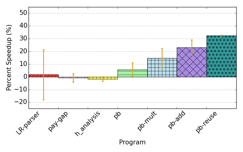
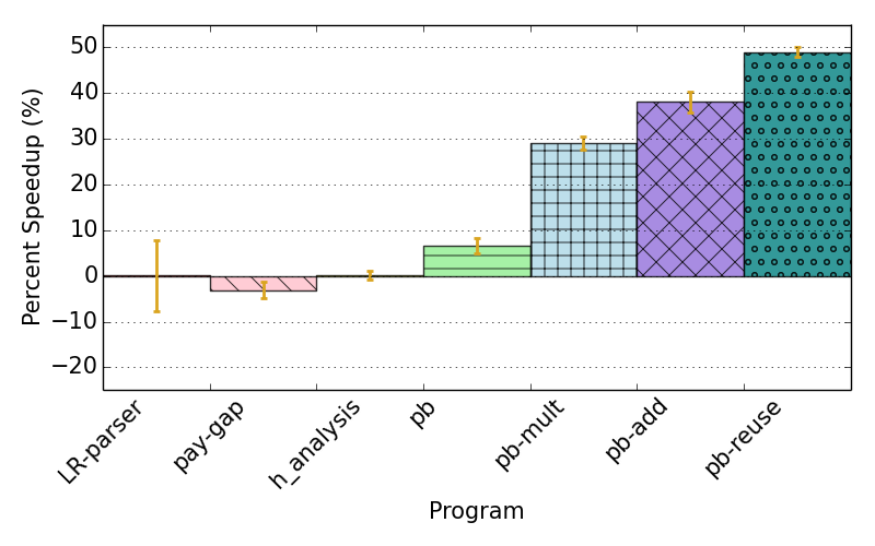
Refer to caption
(a) Local
Refer to caption
(b) Distributed
Figure 10: Percentage Runtime Differences

8 Conclusions

22 avgFemaleSalPub=smcopen(avgFemaleSalary);
23 femaleCountPub=smcopen(femaleCount);
24 avgMaleSalPub=smcopen(avgMaleSalary); maleCountPub=smcopen(maleCount);
25 avgFemaleSalPub=(avgFemaleSalPub/femaleCountPub)/2+historicFemaleSalAvg/2;
26 avgMaleSalPub=(avgMaleSalPub/maleCountPub)/2+historicMaleSalAvg/2;
27
28 for (i=1; i<numParticipants+1; i++)
29 smcoutput(avgFemaleSalPub, i); smcoutput(avgMaleSalPub, i);
Figure 11: Securely calculating the gender pay gap for 100 organizations with additional information released.

In this paper we have presented a formal model for a general SMC compiler, supporting both safe and unsafe features of C. Our model does not artificially restrict what C features can be present in private branches – restrictions are instead guided by which operations our model has shown to be unsafe. Our extension supports additional tracking meta-data to provide support for features unsafe in current SMC techniques. The intuition, shown in our motivation, is that state-of-the-art SMC techniques cannot track complex memory indirections that can occur when using pointers. By providing this tracking, these operations can be made safe. As future work we plan on extending our model to support explicit declassification, through a primitive PICCO calls smcopen. Consider Figure 11 which highlights a modification to our original gender based salary computation (lines 16-17) from Figure 1. Explicitly declassifying the sum and count earlier in the program, allows us to change the average computation to a public computation. This reduces the number of high cost communications and cryptographic computations in the program. To support explicit declassification in our model we would need to extend our semantics with gradual release [3].

Acknowledgements

This work was supported in part by a Google Faculty Research Award and US National Science Foundation grants 1749539, 1845803, 2040249, and 2213057. Any opinions, findings, and conclusions or recommendations expressed in this publication are those of the authors and do not necessarily reflect the views of the funding sources.

References

  • [1] M. Abadi, A. Banerjee, N. Heintze, and J. Riecke. A core calculus of dependency. In ACM SIGPLAN-SIGACT Symposium on Principles of Programming Languages (POPL), pages 147–160, 1999.
  • [2] C. Abate, R. Blanco, Ş. Ciobâcă, A. Durier, D. Garg, C. Hritcu, M. Patrignani, É. Tanter, and J. Thibault. Trace-relating compiler correctness and secure compilation. In European Symposium on Programming(ESOP), pages 1–28, 2020.
  • [3] Aslan Askarov and Andrei Sabelfeld. Gradual release: Unifying declassification, encryption and key release policies. In 2007 IEEE Symposium on Security and Privacy (S&P 2007), 20-23 May 2007, Oakland, California, USA, pages 207–221. IEEE Computer Society, 2007.
  • [4] T. Austin and C. Flanagan. Efficient purely-dynamic information flow analysis. In Workshop on Programming Languages and Analysis for Security (PLAS), pages 113–124, 2009.
  • [5] A. Ben-David, N. Nisan, and B. Pinkas. FairplayMP: A system for secure multi-party computation. In ACM Conference on Computer and Communications Security (CCS), pages 257–266, 2008.
  • [6] R. Bendlin, I. Damgard, C. Orlandi, and S. Zakarias. Semi-homomorphic encryption and multiparty computation. In Advances in Cryptography – EUROCRYPT, pages 169–188, 2011.
  • [7] D. Bogdanov, S. Laur, and J. Willemson. Sharemind: A framework for fast privacy-preserving computations. In European Symposium on Research in Computer Security (ESORICS), pages 192–206, 2008.
  • [8] I. Damgård, M. Geisler, M. Krøigaard, and J. Nielsen. Asynchronous multiparty computation: Theory and implementation. In Public Key Cryptography (PKC), pages 160–179, 2009.
  • [9] I. Damgard, V. Pastro, N. Smart, and S. Zakarias. Multiparty computation from somewhat homomorphic encryption. In Advances in Cryptology – CRYPTO, pages 643–662, 2012.
  • [10] D. Demmler, T. Schneider, and M. Zohner. ABY – A framework for efficient mixed-protocol secure two-party computation. In Network and Distributed System Secuity Symposium (NDSS), 2015.
  • [11] D. Devriese and F. Piessens. Noninterference through secure multi-execution. In IEEE Symposium on Security and Privacy (S&P), pages 109–124, 2010.
  • [12] T. ElGamal. A public key cryptosystem and a signature scheme based on discrete logarithms. IEEE Transactions on Information Theory, 31(4):469–472, 1985.
  • [13] B. Ford. Plugging side-channel leaks with timing information flow control. In USENIX Workshop on Hot Topics in Cloud Computing (HotCloud), 2012.
  • [14] R. Gennaro, M. Rabin, and T. Rabin. Simplified VSS and fast-track multiparty computations with applications to threshold cryptography. In ACM Symposium on Principles of Distributed Computing (PODC), pages 101–111, 1998.
  • [15] M. Hastings, B. Hemenway, D. Noble, and S. Zdancewic. SoK: General purpose compilers for secure multi-party computation. In IEEE Symposium on Security and Privacy (S&P), pages 1220–1237, 2019.
  • [16] W. Henecka, A.-R. Sadeghi, T. Schneider, and I. Wehrenberg. TASTY: Tool for automating secure two-party computations. In ACM Conference on Computer and Communications Security (CCS), pages 451–462, 2010.
  • [17] A. Holzer, M. Franz, S. Katzenbeisser, and H. Veith. Secure two-party computations in ANSI C. In ACM Conference on Computer and Communications Security (CCS), pages 772–783, 2012.
  • [18] R. Jagomägis. SecreC: A privacy-aware programming language with applications in data mining. Master’s thesis, University of Tartu, 2010.
  • [19] B. Kreuter, a. shelat, B. Mood, and K. Butler. PCF: A portable circuit format for scalable two-party secure computation. In USENIX Security Symposium, pages 321–336, 2013.
  • [20] A. Lapets, F. Jansen, K. Albab, R. Issa, L. Qin, M. Varia, and A. Bestavros. Accessible privacy-preserving web-based data analysis for assessing and addressing economic inequalities. In ACM SIGCAS Conference on Computing and Sustainable Societies (COMPASS), 2018.
  • [21] P. Laud and A. Pankova. Optimizing secure computation programs with private conditionals. In International Conference on Information and Communications Security (ICICS), pages 418–430, 2016.
  • [22] X. Leroy, A. Appel, S. Blazy, and G. Stewart. The CompCert memory model, Version 2. Technical Report RR-7987, INRIA, 2012.
  • [23] C. Liu, Y. Huang, E. Shi, J. Katz, and M. Hicks. Automating efficient RAM-model secure computation. In IEEE Symposiym on Security and Privacy (S&P), pages 623–638, 2014.
  • [24] C. Liu, X. Wang, K. Nayak, Y. Huang, and E. Shi. ObliVM: A programming framework for secure computation. In IEEE Symposium on Security and Privacy (S&P), 2015.
  • [25] D. Malkhi, N. Nisan, B. Pinkas, and Y. Sella. Fairplay – Secure two-party computation system. In USENIX Security Symposium, 2004.
  • [26] J. Mitchell, R. Sharma, D. Stefan, and J. Zimmerman. Information-flow control for programming on encrypted data. In IEEE Computer Security Foundations Symposium (CSF), pages 45–60, 2012.
  • [27] B. Mood, D. Gupta, H. Carter, K. Butler, and P. Traynor. Frigate: A validated, extensible, and efficient compiler and interpreter for secure computation. In IEEE European Symposium on Security and Privacy (Euro S&P), 2016.
  • [28] J. Nielsen, P. Nordholt, C. Orlandi, and S. Burra. A new approach to practical active-secure two-party computation. In Advances in Cryptology – CRYPTO, pages 681–700, 2012.
  • [29] P. Paillier. Public-key cryptosystems based on composite degree residuosity classes. In Advances in Cryptology – EUROCRYPT, pages 223–238, 1999.
  • [30] M. Patrignani and D. Garg. Secure compilation and hyperproperty preservation. In IEEE Computer Security Foundations Symposium (CSF), pages 392–404, 2017.
  • [31] M. Pettai and P. Laud. Automatic proofs of privacy of secure multi-party computation protocols against active adversaries. In IEEE Computer Security Foundations Symposium (CSF), pages 75–89, 2015.
  • [32] J. Planul and J. Mitchell. Oblivious program execution and path-sensitive non-interference. In IEEE Computer Security Foundations Symposium (CSF), pages 66–80, 2013.
  • [33] A. Rastogi, M. Hammer, and M. Hicks. Wysteria: A programming language for generic, mixed-mode multiparty computations. In IEEE Symposium on Security and Privacy, pages 655–670, 2014.
  • [34] A. Rastogi, N. Swamy, and M. Hicks. WYS*: A DSL for verified secure multi-party computations. In International Conferece on Principles of Security and Trust (POST), pages 99–122, 2019.
  • [35] Amy Rathore. A Formal Model for a General-Purpose Compiler for Secure Multiparty Computations. PhD thesis, University at Buffalo, 2022.
  • [36] A. Sabelfeld and A. Russo. From dynamic to static and back: Riding the roller coaster of information-flow control research. In Perspectives of Systems Informatics (PSI), pages 352–365, 2009.
  • [37] A. Shamir. How to share a secret. Communications of the ACM, 22(11):612–613, 1979.
  • [38] V. Sokk. An improved type system for a privacy-aware programming language and its practical applications. Master’s thesis, University of Tartu, 2016.
  • [39] E. Songhori, S. Hussain, A.-R. Sadeghi, T. Schneider, and F. Koushanfar. TinyGarble: Highly compressed and scalable sequential garbled circuits. In IEEE Symposium on Security and Privacy, pages 411–428, 2015.
  • [40] D. Volpano and G. Smith. A type-based approach to program security. In International Joint Conference CAAP/FASE on Theory and Practice of Software Development (TAPSOFT), pages 607–621, 1997.
  • [41] A. Yao. How to generate and exchange secrets. In IEEE Symposium on Foundations of Computer Science, pages 162–167, 1986.
  • [42] Y. Zhang, M. Blanton, and G. Almashaqbeh. Implementing support for pointers to private data in a general-purpose secure multi-party compiler. ACM Transactions on Privacy and Security (TOPS), 21(2), 2018.
  • [43] Y. Zhang, A. Steele, and M. Blanton. PICCO: A general-purpose compiler for private distributed computation. In ACM Conference on Computer and Communications Security (CCS), pages 813–826, 2013.

Appendix A Multiparty Protocols

Algorithm 2, MPCb\mathrm{MPC}_{\mathit{{b}}}, is a selection control algorithm that directs the evaluation to the relevant multiparty computation algorithm based on the given binary operation 𝑏𝑜𝑝∈{⋅,÷,+,−}\mathit{bop}\in\{\cdot,\div,+,-\}.

Algorithm 2 (n31,…,n3q)←MPCb​(𝑏𝑜𝑝,[n11,…,n1q],[n21,…,n2q])(n^{\mathrm{{1}}}_{3},...,n^{\mathrm{{q}}}_{3})\leftarrow\mathrm{MPC}_{\mathit{{b}}}(\mathit{bop},[n^{\mathrm{{1}}}_{1},...,n^{\mathrm{{q}}}_{1}],[n^{\mathrm{{1}}}_{2},...,n^{\mathrm{{q}}}_{2}])
 if (𝑏𝑜𝑝=⋅)(\mathit{bop}=\cdot) then
   for all p∈{1​…​q}\mathrm{{p}}\in\{\mathrm{{1}}...\mathrm{{q}}\} do
   n3p=MPC𝑚𝑢𝑙𝑡​(n1p,n2p)n^{\mathrm{{p}}}_{3}=\mathrm{MPC}_{\mathit{{mult}}}(n^{\mathrm{{p}}}_{1},n^{\mathrm{{p}}}_{2})
   end for
   return (n31,…,n3q)(n^{\mathrm{{1}}}_{3},...,n^{\mathrm{{q}}}_{3})
 else if (𝑏𝑜𝑝=÷)(\mathit{bop}=\div) then
   for all p∈{1​…​q}\mathrm{{p}}\in\{\mathrm{{1}}...\mathrm{{q}}\} do
   n3p=MPC𝑑𝑖𝑣​(n1p,n2p)n^{\mathrm{{p}}}_{3}=\mathrm{MPC}_{\mathit{{div}}}(n^{\mathrm{{p}}}_{1},n^{\mathrm{{p}}}_{2})
   end for
   return (n31,…,n3q)(n^{\mathrm{{1}}}_{3},...,n^{\mathrm{{q}}}_{3})
 else if (𝑏𝑜𝑝=−)(\mathit{bop}=-) then
   for all p∈{1​…​q}\mathrm{{p}}\in\{\mathrm{{1}}...\mathrm{{q}}\} do
   n3p=MPC𝑠𝑢𝑏​(n1p,n2p)n^{\mathrm{{p}}}_{3}=\mathrm{MPC}_{\mathit{{sub}}}(n^{\mathrm{{p}}}_{1},n^{\mathrm{{p}}}_{2})
   end for
   return (n31,…,n3q)(n^{\mathrm{{1}}}_{3},...,n^{\mathrm{{q}}}_{3})
 else if (𝑏𝑜𝑝=+)(\mathit{bop}=+) then
   for all p∈{1​…​q}\mathrm{{p}}\in\{\mathrm{{1}}...\mathrm{{q}}\} do
   n3p=MPC𝑎𝑑𝑑​(n1p,n2p)n^{\mathrm{{p}}}_{3}=\mathrm{MPC}_{\mathit{{add}}}(n^{\mathrm{{p}}}_{1},n^{\mathrm{{p}}}_{2})
   end for
   return (n31,…,n3q)(n^{\mathrm{{1}}}_{3},...,n^{\mathrm{{q}}}_{3})
 end if

Each of the given multiparty protocols in Algorithm 2 (i.e., MPC𝑚𝑢𝑙𝑡,\mathrm{MPC}_{\mathit{{mult}}}, MPC𝑠𝑢𝑏,\mathrm{MPC}_{\mathit{{sub}}}, MPC𝑎𝑑𝑑,\mathrm{MPC}_{\mathit{{add}}}, MPC𝑑𝑖𝑣\mathrm{MPC}_{\mathit{{div}}}) must be defined using protocols that have been proven to uphold the desired properties within our proofs (i.e., correctness and noninterference). We give an example definition for MPC𝑚𝑢𝑙𝑡\mathrm{MPC}_{\mathit{{mult}}} in Algorithm 1, but this definition can be swapped out with any protocol for the secure multiparty computation of multiplication that maintains the properties of correctness and noninterference. We defer the definition of all other SMC binary operations, rely on assertions that the protocols chosen to be used with this model will maintain both correctness and noninterference in our proofs. We chose this strategy as SMC implementations of such protocols will be proven to hold our desired properties on their own, and this allows us to not only leverage those proofs, but to also improve the versatility of our model by allowing such algorithms to be easily swapped out as newer, improved versions become available.

Appendix B Semantics

Private Array Declaration
(e)⊬γ((𝑡𝑦=private​𝑏𝑡𝑦)∨(𝑡𝑦=𝑏𝑡𝑦))∧((𝑏𝑡𝑦=int)∨(𝑏𝑡𝑦=float))((p,γ,σ,Δ,acc,e)∥C)⇓ℒ1𝒟1((p,γ,σ1,Δ,acc,α)∥C1)α>0ω=EncodePtr(privateconst𝑏𝑡𝑦∗,[1,[(l1,0)],[1], 1])l=ϕ⁡()ω1=EncodeArr⁡(private​𝑏𝑡𝑦,α,NULL)l1=ϕ⁡()γ1=γ[x→(l,privateconst𝑏𝑡𝑦∗)]σ2=σ1[l→(ω,privateconst𝑏𝑡𝑦∗,1,PermL_Ptr(Freeable,privateconst𝑏𝑡𝑦∗,private,1))]σ3=σ2[l1→(ω1,private𝑏𝑡𝑦,α,PermL(Freeable,private𝑏𝑡𝑦,private,α))]((p,γ,σ,Δ,acc,𝑡𝑦x[e])∥C)⇓ℒ1::(p,[(l,0),(l1,0)])𝒟1::(p,[da1])((p,γ1,σ3,Δ,acc,skip)∥C1)\frac{\begin{array}[]{l}\begin{array}[]{l l}({e})\nvdash{\color[rgb]{1,0,0}\gamma}&((\mathit{ty}={\mathrm{private}\ \mathit{bty}})\lor(\mathit{ty}={\mathit{bty}}))\land((\mathit{bty}=\mathrm{int})\lor(\mathit{bty}=\mathrm{float}))\crcr&((\mathrm{{p}},{\color[rgb]{1,0,0}\gamma},\ \sigma,\ {\Delta},\ \mathrm{acc},\ e)\-\ \|\ C)\Downarrow^{\mathcal{L}_{1}}_{\mathit{\mathcal{D}_{1}}}((\mathrm{{p}},{\color[rgb]{1,0,0}\gamma},\ \sigma{{}_{1}},\ {\Delta},\ \mathrm{acc},\ \alpha)\-\ \|\ C_{1})\crcr\alpha>0&\omega=\mathrm{EncodePtr}({\mathrm{private}\ \mathrm{const}\ \mathit{bty}*},\ [1,\ [({l_{1}},0)],\ [1],\ 1])\crcr{l}=\phi()&\omega_{1}=\mathrm{EncodeArr}(\mathrm{private}\ \mathit{bty},\alpha,\mathrm{NULL})\crcr{l_{1}}=\phi()&{\color[rgb]{1,0,0}\gamma{{}_{1}}=\gamma[x\ \to\ (l,\ {\mathrm{private}\ \mathrm{const}\ \mathit{bty}*})]}\end{array}\crcr\begin{array}[]{l}\sigma{{}_{2}}=\sigma{{}_{1}}[{l}\to(\omega,{\mathrm{private}\ \mathrm{const}\ \mathit{bty}*},1,\mathrm{PermL}\_\mathrm{Ptr}(\mathrm{Freeable},{\mathrm{private}\ \mathrm{const}\ \mathit{bty}*},\mathrm{private},1))]\crcr\sigma{{}_{3}}=\sigma{{}_{2}}[{l_{1}}\to(\omega_{1},\ {\mathrm{private}\ \mathit{bty}},\ \alpha,\ \mathrm{PermL}(\mathrm{Freeable},\mathrm{private}\ \mathit{bty},\mathrm{private},\alpha))]\end{array}\end{array}}{((\mathrm{{p}},{\color[rgb]{1,0,0}\gamma},\ \sigma,\ {\Delta},\ \mathrm{acc},\ {\mathit{ty}\ x[e]})\-\ \|\ C)\ \Downarrow^{\mathcal{L}_{1}::(\mathrm{{p}},[(l,0),({l_{1}},0)])}_{\mathit{\mathcal{D}_{1}::(\mathrm{{p}},[\mathit{da1}])}}((\mathrm{{p}},{\color[rgb]{1,0,0}\gamma{{}_{1}}},\ \sigma{{}_{3}},\ {\Delta},\ \mathrm{acc},\ \mathrm{skip})\-\ \|\ C_{1})}
Statement Sequencing
((p,γ,σ,Δ,acc,s1)∥C)⇓ℒ1𝒟1((p,γ1,σ1,Δ1,acc,v1)∥C1)((p,γ1,σ1,Δ1,acc,s2)∥C1)⇓ℒ2𝒟2((p,γ2,σ2,Δ2,acc,v2)∥C2)((p,γ,σ,Δ,acc,s1;s2)∥C)⇓ℒ1::ℒ2𝒟1::𝒟2::(p,[𝑠𝑠])((p,γ2,σ2,Δ2,acc,v)∥C2)\frac{\begin{array}[]{l}((\mathrm{{p}},\ {\color[rgb]{1,0,0}\gamma},\ \sigma,\ {\Delta},\ \mathrm{acc},{s_{1}})\-\ \|\ C)\ \Downarrow^{\mathcal{L}_{1}}_{\mathit{\mathcal{D}_{1}}}((\mathrm{{p}},{\color[rgb]{1,0,0}\gamma{{}_{1}}},\sigma{{}_{1}},{\Delta_{1}},\mathrm{acc},v_{1})\-\ \|\ C_{1})\crcr((\mathrm{{p}},{\color[rgb]{1,0,0}\gamma{{}_{1}}},\sigma{{}_{1}},{\Delta_{1}},\mathrm{acc},{s_{2}})\-\ \|\ C_{1})\Downarrow^{\mathcal{L}_{2}}_{\mathit{\mathcal{D}_{2}}}((\mathrm{{p}},{\color[rgb]{1,0,0}\gamma{{}_{2}}},\sigma{{}_{2}},{\Delta_{2}},\mathrm{acc},v_{2})\-\ \|\ C_{2})\end{array}}{((\mathrm{{p}},{\color[rgb]{1,0,0}\gamma},\ \sigma,\ {\Delta},\ \mathrm{acc},\ {s_{1};\ s_{2}})\-\ \|\ C)\Downarrow^{\mathcal{L}_{1}::\mathcal{L}_{2}}_{\mathit{\mathcal{D}_{1}::\mathcal{D}_{2}::(\mathrm{{p}},[\mathit{ss}])}}((\mathrm{{p}},{\color[rgb]{1,0,0}\gamma{{}_{2}}},\ \sigma{{}_{2}},\ {\Delta_{2}},\ \mathrm{acc},\ {v})\-\ \|\ C_{2})}
Public If Else True
(e)⊬γ((p,γ,σ,Δ,acc,e)∥C)⇓ℒ1𝒟1((p,γ,σ1,Δ1,acc,n)∥C1)n≠ 0((p,γ,σ1,Δ1,acc,s1)∥C1)⇓ℒ2𝒟2((p,γ1,σ2,Δ2,acc,skip)∥C2)((p,γ,σ,Δ,acc,if(e)s1elses2)∥C)⇓ℒ1::ℒ2𝒟1::𝒟2::(p,[𝑖𝑒𝑡])((p,γ,σ2,Δ2,acc,skip)∥C2)\frac{\begin{array}[]{l l}(e)\nvdash{\color[rgb]{1,0,0}\gamma}&((\mathrm{{p}},{\color[rgb]{1,0,0}\gamma},\ \sigma,\ {\Delta},\ \mathrm{acc},e)\ \ \-\ \|\ C)\ \Downarrow^{\mathcal{L}_{1}}_{\mathit{\mathcal{D}_{1}}}((\mathrm{{p}},{\color[rgb]{1,0,0}\gamma},\ \sigma{{}_{1}},{\Delta_{1}},\mathrm{acc},n)\hskip 8.50012pt\ \-\ \|\ C_{1})\crcr n\ \neq\ 0&((\mathrm{{p}},{\color[rgb]{1,0,0}\gamma},\sigma{{}_{1}},{\Delta_{1}},\mathrm{acc},{s_{1}})\-\ \|\ C_{1})\Downarrow^{\mathcal{L}_{2}}_{\mathit{\mathcal{D}_{2}}}((\mathrm{{p}},{\color[rgb]{1,0,0}\gamma{{}_{1}}},\sigma{{}_{2}},{\Delta_{2}},\mathrm{acc},\mathrm{skip})\-\ \|\ C_{2})\end{array}}{((\mathrm{{p}},{\color[rgb]{1,0,0}\gamma},\ \sigma,\ {\Delta},\ \mathrm{acc},\ {\mathrm{if}\ (e)\ s_{1}\ \mathrm{else}\ s_{2}})\-\ \|\ C)\ \Downarrow^{\mathcal{L}_{1}::\mathcal{L}_{2}}_{\mathit{\mathcal{D}_{1}::\mathcal{D}_{2}::(\mathrm{{p}},[\mathit{iet}])}}((\mathrm{{p}},{\color[rgb]{1,0,0}\gamma},\ \sigma{{}_{2}},\ {\Delta_{2}},\ \mathrm{acc},\ \mathrm{skip})\-\ \|\ C_{2})}
Figure 12: An illustration of scoping within SMC2 rules. We highlight the environment γ{\color[rgb]{1,0,0}\gamma} and its modifications in red.
Public Multiplication
(e1,e2)⊬γ((p,γ,σ,Δ,acc,e1)∥C)⇓ℒ1𝒟1((p,γ,σ1,Δ1,acc,n1)∥C1)((p,γ,σ1,Δ1,acc,e2)∥C1)⇓ℒ2𝒟2((p,γ,σ2,Δ2,acc,n2)∥C2)n1⋅n2=n3((p,γ,σ,Δ,acc,e1⋅e2)∥C)⇓ℒ1::ℒ2𝒟1::𝒟2::(p,[𝑏𝑚])((p,γ,σ2,Δ2,acc,n3)∥C2)\frac{\begin{array}[]{l}({e_{1}},{e_{2}})\nvdash\gamma\hskip 17.00024pt\hskip 17.00024pt\hskip 8.50012pt((\mathrm{{p}},\gamma,\ \sigma,\ {\Delta},\ \mathrm{acc},\ {e_{1}})\-\ \|\ C)\ \Downarrow^{\mathcal{L}_{1}}_{\mathit{\mathcal{D}_{1}}}((\mathrm{{p}},\gamma,\ \sigma{{}_{1}},\ {\Delta_{1}},\ \mathrm{acc},\ {n_{1}})\-\ \|\ C_{1})\crcr((\mathrm{{p}},\gamma,\ \sigma{{}_{1}},\ {\Delta_{1}},\ \mathrm{acc},\ {e_{2}})\-\ \|\ C_{1})\ \Downarrow^{\mathcal{L}_{2}}_{\mathit{\mathcal{D}_{2}}}((\mathrm{{p}},\gamma,\ \sigma{{}_{2}},\ {\Delta_{2}},\ \mathrm{acc},\ {n_{2}})\-\ \|\ C_{2})\hskip 17.00024pt\hskip 17.00024pt{n_{1}}\cdot{n_{2}}={n_{3}}\end{array}}{((\mathrm{{p}},\gamma,\ \sigma,\ {\Delta},\ \mathrm{acc},\ {e_{1}\cdot e_{2}})\-\ \|\ C)\ \Downarrow^{\mathcal{L}_{1}::\mathcal{L}_{2}}_{\mathit{\mathcal{D}_{1}::\mathcal{D}_{2}::(\mathrm{{p}},[\mathit{bm}])}}((\mathrm{{p}},\gamma,\ \sigma{{}_{2}},\ {\Delta_{2}},\ \mathrm{acc},\ {n_{3}})\-\ \|\ C_{2})}
Read Private Variable
γ⁡(x)=(l,private​𝑏𝑡𝑦)σ⁡(l)=(ω,private​𝑏𝑡𝑦, 1,PermL⁡(Freeable,private​𝑏𝑡𝑦,private,1))DecodeVal⁡(private​𝑏𝑡𝑦,ω)=n((p,γ,σ,Δ,acc,x)∥C)⇓(p,[(l,0)])(p,[r1])((p,γ,σ,Δ,acc,n)∥C)\frac{\begin{array}[]{l l}\gamma(x)=(l,\ \mathrm{private}\ \mathit{bty})&\sigma(l)=(\omega,\ \mathrm{private}\ \mathit{bty},\ 1,\ \mathrm{PermL}(\mathrm{Freeable},\mathrm{private}\ \mathit{bty},\mathrm{private},1))\crcr&\mathrm{DecodeVal}(\mathrm{private}\ \mathit{bty},\ \omega)=n\end{array}}{((\mathrm{{p}},\gamma,\ \sigma,\ {\Delta},\ \mathrm{acc},\ x)\-\ \|\ C)\ \Downarrow^{(\mathrm{{p}},[(l,0)])}_{\mathit{(\mathrm{{p}},[\mathit{r1}])}}((\mathrm{{p}},\gamma,\ \sigma,\ {\Delta},\ \mathrm{acc},\ n)\-\ \|\ C)}
Public Malloc
acc=0(e)⊬γ((p,γ,σ,Δ,acc,e)∥C)⇓ℒ1𝒟1((p,γ,σ1,Δ,acc,n)∥C1)l=ϕ⁡()σ2=σ1[l→(NULL,void∗,n,PermL(Freeable,void∗,public,n))]((p,γ,σ,Δ,acc,malloc(e))∥C)⇓ℒ1::(p,[(l,0)])𝒟1::(p,[𝑚𝑎𝑙])((p,γ,σ2,Δ,acc,(l,0))∥C1)\frac{\begin{array}[]{l l l}\mathrm{acc}=0&(e)\nvdash\gamma&((\mathrm{{p}},\gamma,\ \sigma,\ {\Delta},\ \mathrm{acc},\ e)\-\ \|\ C)\ \Downarrow^{\mathcal{L}_{1}}_{\mathit{\mathcal{D}_{1}}}((\mathrm{{p}},\gamma,\ \sigma{{}_{1}},\ {\Delta},\ \mathrm{acc},\ n)\-\ \|\ C_{1})\crcr l=\phi()&&\sigma_{2}=\sigma_{1}\big[l\to\big(\mathrm{NULL},\mathrm{void}*,n,\mathrm{PermL}(\mathrm{Freeable},\mathrm{void}*,\mathrm{public},n)\big)\big]\end{array}}{\begin{array}[]{l}((\mathrm{{p}},\gamma,\ \sigma,\ {\Delta},\ \mathrm{acc},\ \mathrm{malloc}(e))\-\ \|\ C)\Downarrow^{\mathcal{L}_{1}::(\mathrm{{p}},[(l,0)])}_{\mathit{\mathcal{D}_{1}::(\mathrm{{p}},[\mathit{mal}])}}((\mathrm{{p}},\gamma,\ \sigma{{}_{2}},\ {\Delta},\ \mathrm{acc},\ (l,0))\-\ \|\ C_{1})\end{array}}
Public Free
γ(x)=(l,public𝑏𝑡𝑦∗)σ(l)=(ω,public𝑏𝑡𝑦∗,1,PermL(Freeable,public𝑏𝑡𝑦∗,public,1))acc=0DecodePtr(public𝑏𝑡𝑦∗, 1,ω)=[1,[(l1,0)],[1], 1]CheckFreeable⁡(γ,[(l1,0)],[1],σ)=1Free(σ,l1)=(σ1,(l1,0))((p,γ,σ,Δ,acc,free(x))∥C)⇓(p,[(l,0),(l1,0)])(p,[𝑓𝑟𝑒])((p,γ,σ1,Δ,acc,skip)∥C)\frac{\begin{array}[]{l}\begin{array}[]{l l}\gamma(x)=(l,\ {\mathrm{public}\ \mathit{bty}*})&\sigma(l)=(\omega,\mathrm{public}\ \mathit{bty}*,1,\mathrm{PermL}(\mathrm{Freeable},\mathrm{public}\ \mathit{bty}*,\mathrm{public},1))\crcr\mathrm{acc}=0&\mathrm{DecodePtr}({\mathrm{public}\ \mathit{bty}*},\ 1,\ \omega)=[1,\ [({l_{1}},0)],\ [1],\ 1]\end{array}\crcr\begin{array}[]{l l}\mathrm{CheckFreeable}(\gamma,[({l_{1}},0)],[1],\sigma)=1&\mathrm{Free}(\sigma,\ l_{1})=(\sigma{{}_{1}},(l_{1},0))\end{array}\end{array}}{((\mathrm{{p}},\gamma,\ \sigma,\ {\Delta},\ \mathrm{acc},\ {\mathrm{free}(x)})\-\ \|\ C)\ \Downarrow^{(\mathrm{{p}},[(l,0),(l_{1},0)])}_{\mathit{(\mathrm{{p}},[\mathit{fre}])}}((\mathrm{{p}},\gamma,\ \sigma{{}_{1}},\ {\Delta},\ \mathrm{acc},\ \mathrm{skip})\-\ \|\ C)}
SMC Input Public Value
(e)⊬γ((p,γ,σ,Δ,acc,e)∥C)⇓ℒ1𝒟1((p,γ,σ1,Δ1,acc,n)∥C1)γ⁡(x)=(l,public​𝑏𝑡𝑦)InputValue⁡(x,n)=n1acc=0((p,γ,σ1,Δ1,acc,x=n1)∥C1)⇓ℒ2𝒟2((p,γ,σ2,Δ2,acc,skip)∥C2)((p,γ,σ,Δ,acc,smcinput(x,e))∥C)⇓ℒ1::ℒ2𝒟1::𝒟2::(p,[𝑖𝑛𝑝])((p,γ,σ2,Δ2,acc,skip)∥C2)\frac{\begin{array}[]{l l}({e})\nvdash\gamma&((\mathrm{{p}},\gamma,\sigma,{\Delta},\mathrm{acc},{e})\-\ \|\ C)\ \Downarrow^{\mathcal{L}_{1}}_{\mathit{\mathcal{D}_{1}}}((\mathrm{{p}},\gamma,\sigma{{}_{1}},{\Delta_{1}},\mathrm{acc},{n})\hskip 8.50012pt\-\ \|\ C_{1})\crcr\gamma(x)=(l,\mathrm{public}\ \mathit{bty})&\mathrm{InputValue}(x,{n})={n_{1}}\crcr\mathrm{acc}=0&((\mathrm{{p}},\gamma,\sigma{{}_{1}},{\Delta_{1}},\mathrm{acc},{x=n_{1}})\-\ \|\ C_{1})\Downarrow^{\mathcal{L}_{2}}_{\mathit{\mathcal{D}_{2}}}((\mathrm{{p}},\gamma,\sigma{{}_{2}},{\Delta_{2}},\mathrm{acc},\mathrm{skip})\-\ \|\ C_{2})\end{array}}{((\mathrm{{p}},\gamma,\ \sigma,\ {\Delta},\ \mathrm{acc},\ {\mathrm{smcinput}(x,\ e)})\-\ \|\ C)\Downarrow^{\mathcal{L}_{1}::\mathcal{L}_{2}}_{\mathit{\mathcal{D}_{1}::\mathcal{D}_{2}::(\mathrm{{p}},[\mathit{inp}])}}((\mathrm{{p}},\gamma,\ \sigma{{}_{2}},\ {\Delta_{2}},\ \mathrm{acc},\ \mathrm{skip})\-\ \|\ C_{2})}
SMC Output Private Array
(e1,e2)⊬γ((p,γ,σ,Δ,acc,e1)∥C)⇓ℒ1𝒟1((p,γ,σ1,Δ1,acc,n)∥C1)γ(x)=(l,privateconst𝑏𝑡𝑦∗)((p,γ,σ1,Δ1,acc,e2)∥C1)⇓ℒ2𝒟2((p,γ,σ2,Δ2,acc,α)∥C2)σ2(l)=(ω,privateconst𝑏𝑡𝑦∗,1,PermL_Ptr(Freeable,privateconst𝑏𝑡𝑦∗,private,1))DecodePtr(privateconst𝑏𝑡𝑦∗, 1,ω)=[1,[(l1,0)],[1],private𝑏𝑡𝑦, 1]σ2(l1)=(ω1,private𝑏𝑡𝑦,α,PermL(Freeable,private𝑏𝑡𝑦,private,α))∀i∈{0,…,α−1}DecodeArr⁡(private​𝑏𝑡𝑦,i,ω1)=miOutputArray⁡(x,n,[m0,…,mα−1])((p,γ,σ,Δ,acc,smcoutput(x,e1,e2))∥C)⇓ℒ1::ℒ2::(p,[(l,0),(l1,0),…,(l1,n1−1)])𝒟1::𝒟2::(p,[out3])((p,γ,σ2,Δ2,acc,skip)∥C2)\frac{\begin{array}[]{l}\begin{array}[]{l l}({e_{1}},{e_{2}})\nvdash\gamma&((\mathrm{{p}},\gamma,\ \sigma,\ {\Delta},\ \mathrm{acc},{e_{1}})\-\ \|\ C)\ \Downarrow^{\mathcal{L}_{1}}_{\mathit{\mathcal{D}_{1}}}((\mathrm{{p}},\gamma,\sigma{{}_{1}},{\Delta_{1}},\mathrm{acc},{n})\-\ \|\ C_{1})\crcr\gamma(x)=({l},{\mathrm{private}\ \mathrm{const}\ \mathit{bty}*})&((\mathrm{{p}},\gamma,\sigma{{}_{1}},{\Delta_{1}},\mathrm{acc},{e_{2}})\-\ \|\ C_{1})\Downarrow^{\mathcal{L}_{2}}_{\mathit{\mathcal{D}_{2}}}((\mathrm{{p}},\gamma,\sigma{{}_{2}},{\Delta_{2}},\mathrm{acc},{\alpha})\-\ \|\ C_{2})\end{array}\crcr\begin{array}[]{l}\sigma{{}_{2}}({l})=({\omega},{\mathrm{private}\ \mathrm{const}\ \mathit{bty}*},1,\mathrm{PermL}\_\mathrm{Ptr}(\mathrm{Freeable},{\mathrm{private}\ \mathrm{const}\ \mathit{bty}*},\mathrm{private},1))\crcr\mathrm{DecodePtr}({\mathrm{private}\ \mathrm{const}\ \mathit{bty}*},\ 1,\ {\omega})=[1,\ [({l_{1}},0)],\ [1],\ \mathrm{private}\ \mathit{bty},\ 1]\crcr\sigma{{}_{2}}({l_{1}})=({\omega_{1}},\ {\mathrm{private}\ \mathit{bty}},\ {\alpha},\ \mathrm{PermL}(\mathrm{Freeable},\mathrm{private}\ \mathit{bty},\mathrm{private},{\alpha}))\crcr\forall i\in\{0,...,\alpha-1\}\hskip 17.00024pt\mathrm{DecodeArr}({\mathrm{private}\ \mathit{bty}},\ {i},\ {\omega_{1}})={m_{i}}\crcr\mathrm{OutputArray}(x,\ {n},\ [{m_{0}},\ {...},\ {m_{\alpha-1}}])\end{array}\end{array}}{\begin{array}[]{l}((\mathrm{{p}},\gamma,\ \sigma,\ {\Delta},\ \mathrm{acc},\ {\mathrm{smcoutput}(x,\ e_{1},\ e_{2})})\-\ \|\ C)\crcr\Downarrow^{\mathcal{L}_{1}::\mathcal{L}_{2}::(\mathrm{{p}},[(l,0),(l_{1},0),...,(l_{1},n_{1}-1)])}_{\mathit{\mathcal{D}_{1}::\mathcal{D}_{2}::(\mathrm{{p}},[\mathit{out3}])}}((\mathrm{{p}},\gamma,\ \sigma{{}_{2}},\ {\Delta_{2}},\ \mathrm{acc},\ \mathrm{skip})\-\ \|\ C_{2})\end{array}}
Pre-Increment Public Variable
γ⁡(x)=(l,public​𝑏𝑡𝑦)σ⁡(l)=(ω,public​𝑏𝑡𝑦, 1,PermL⁡(Freeable,public​𝑏𝑡𝑦,public,1))acc=0DecodeVal⁡(public​𝑏𝑡𝑦,ω)=nn1=n+1UpdateVal(σ,l,n1,Δ,acc,public𝑏𝑡𝑦)=(σ1,Δ)((p,γ,σ,Δ,acc,++x)∥C)⇓(p,[(l,0)])(p,[𝑝𝑖𝑛])((p,γ,σ1,Δ,acc,n1)∥C)\frac{\begin{array}[]{l l}\gamma(x)=(l,\ \mathrm{public}\ \mathit{bty})&\sigma(l)=(\omega,\ \mathrm{public}\ \mathit{bty},\ 1,\ \mathrm{PermL}(\mathrm{Freeable},\mathrm{public}\ \mathit{bty},\mathrm{public},1))\crcr\mathrm{acc}=0&\mathrm{DecodeVal}(\mathrm{public}\ \mathit{bty},\ \omega)={n}\crcr{n_{1}}={n}+1&\mathrm{UpdateVal}(\sigma,\ l,\ {n_{1}},\ {\Delta},\ \mathrm{acc},\mathrm{public}\ \mathit{bty})=(\sigma{{}_{1}},\ {\Delta})\end{array}}{((\mathrm{{p}},\gamma,\ \sigma,\ {\Delta},\ \mathrm{acc},\ {\mathrel{+}\mathrel{+}x})\-\ \|\ C)\ \Downarrow^{(\mathrm{{p}},[(l,0)])}_{\mathit{(\mathrm{{p}},[\mathit{pin}])}}((\mathrm{{p}},\gamma,\ \sigma{{}_{1}},\ {\Delta},\ \mathrm{acc},\ {n_{1}})\-\ \|\ C)}
Multiparty Private Pointer Dereference Single Level Indirection
{(x)⊢γp}qp=1{γp(x)=(lp,private𝑏𝑡𝑦∗)}qp=1α>1{σp(lp)=(ωp,private𝑏𝑡𝑦∗,α,PermL_Ptr(Freeable,private𝑏𝑡𝑦∗,private,α))}qp=1{DecodePtr(private𝑏𝑡𝑦∗,α,ωp)=[α,Lp,Jp,1]}qp=1{Retrieve_vals(α,Lp,private𝑏𝑡𝑦,σp)=([np0,…npα−1],1)}qp=1MPC𝑑𝑣​([[n01,…,nα−11],…,[n0q,…,nα−1q]],[J1,…,Jq])=(n1,…,nq)((1,γ1,σ1,Δ1,acc,∗x)∥…∥(q,γq,σq,Δq,acc,∗x))⇓(1,(l1,0)::L1)∥…∥(q,(lq,0)::Lq)(ALL,[𝑚𝑝𝑟𝑑𝑝])((1,γ1,σ1,Δ1,acc,n1)​‖…‖​(q,γq,σq,Δq,acc,nq))\frac{\begin{array}[]{l}\{(x)\vdash\gamma^{\mathrm{{p}}}\}^{\mathrm{{q}}}_{\mathrm{{p}}=\mathrm{{1}}}\hskip 17.00024pt\hskip 17.00024pt\{\gamma^{\mathrm{{p}}}(x)=(l^{\mathrm{{p}}},\mathrm{private}\ \mathit{bty}*)\}^{\mathrm{{q}}}_{\mathrm{{p}}=\mathrm{{1}}}\hskip 17.00024pt\hskip 17.00024pt\alpha>1\crcr\{\sigma^{\mathrm{{p}}}(l^{\mathrm{{p}}})=(\omega^{\mathrm{{p}}},\ {\mathrm{private}\ \mathit{bty}*},\ \alpha,\ \mathrm{PermL}\_\mathrm{Ptr}(\mathrm{Freeable},{\mathrm{private}\ \mathit{bty}*},\mathrm{private},\alpha))\}^{\mathrm{{q}}}_{\mathrm{{p}}=\mathrm{{1}}}\crcr\{\mathrm{DecodePtr}({\mathrm{private}\ \mathit{bty}*},\ \alpha,\ \omega^{\mathrm{{p}}})=[\alpha,\ L^{\mathrm{{p}}},\ J^{\mathrm{{p}}},1]\}^{\mathrm{{q}}}_{\mathrm{{p}}=\mathrm{{1}}}\crcr\{\mathrm{Retrieve\_vals}(\alpha,L^{\mathrm{{p}}},\mathrm{private}\ \mathit{bty},\sigma^{\mathrm{{p}}})=([n^{\mathrm{{p}}}_{0},...n^{\mathrm{{p}}}_{\alpha-1}],1)\}^{\mathrm{{q}}}_{\mathrm{{p}}=\mathrm{{1}}}\crcr\mathrm{MPC}_{\mathit{{dv}}}([[n^{\mathrm{{1}}}_{0},...,n^{\mathrm{{1}}}_{\alpha-1}],...,[n^{\mathrm{{q}}}_{0},...,n^{\mathrm{{q}}}_{\alpha-1}]],[J^{\mathrm{{1}}},...,J^{\mathrm{{q}}}])=(n^{\mathrm{{1}}},...,n^{\mathrm{{q}}})\end{array}}{\begin{array}[]{l}((\mathrm{{1}},\gamma^{\mathrm{{1}}},\sigma^{\mathrm{{1}}},\Delta^{\mathrm{{1}}},\mathrm{acc},{*x})\-\ \|\ ...\-\ \|\ (\mathrm{{q}},\gamma^{\mathrm{{q}}},\sigma^{\mathrm{{q}}},\Delta^{\mathrm{{q}}},\mathrm{acc},{*x}))\Downarrow^{(\mathrm{{1}},(l^{\mathrm{{1}}},0)::L^{\mathrm{{1}}})\-\ \|\ ...\-\ \|\ (\mathrm{{q}},(l^{\mathrm{{q}}},0)::L^{\mathrm{{q}}})}_{\mathit{(\mathrm{ALL},[\mathit{mprdp}])}}\crcr((\mathrm{{1}},\gamma^{\mathrm{{1}}},\sigma^{\mathrm{{1}}},\Delta^{\mathrm{{1}}},\mathrm{acc},n^{\mathrm{{1}}})\-\ \|\ ...\-\ \|\ (\mathrm{{q}},\gamma^{\mathrm{{q}}},\sigma^{\mathrm{{q}}},\Delta^{\mathrm{{q}}},\mathrm{acc},n^{\mathrm{{q}}}))\end{array}}
Figure 13: Additional SMC2 semantic rules.
Private Array Read Public Index
(e)⊬γ((p,γ,σ,Δ,acc,e)∥C)⇓ℒ1𝒟1((p,γ,σ1,Δ1,acc,i)∥C1)γ(x)=(l,privateconst𝑏𝑡𝑦∗)σ1(l)=(ω,privateconst𝑏𝑡𝑦∗,1,PermL_Ptr(Freeable,privateconst𝑏𝑡𝑦∗,private,1))DecodePtr(privateconst𝑏𝑡𝑦∗, 1,ω)=[1,[(l1,0)],[1], 1]0≤i≤α−1σ1(l1)=(ω1,private𝑏𝑡𝑦,α,PermL(Freeable,private𝑏𝑡𝑦,private,α))DecodeArr⁡(private​𝑏𝑡𝑦,i,ω1)=ni((p,γ,σ,Δ,acc,x[e])∥C)⇓ℒ1::(p,[(l,0),(l1,i)])𝒟1::(p,[ra1])((p,γ,σ1,Δ1,acc,ni)∥C1)\frac{\begin{array}[]{l}(e)\nvdash\gamma\hskip 17.00024pt\hskip 17.00024pt((\mathrm{{p}},\gamma,\ \sigma,\ {\Delta},\ \mathrm{acc},\ e)\-\ \|\ C)\ \Downarrow^{\mathcal{L}_{1}}_{\mathit{\mathcal{D}_{1}}}((\mathrm{{p}},\gamma,\ \sigma{{}_{1}},\ {\Delta_{1}},\ \mathrm{acc},\ i)\-\ \|\ C_{1})\crcr\gamma(x)=(l,\ {\mathrm{private}\ \mathrm{const}\ \mathit{bty}*})\crcr\sigma{{}_{1}}(l)=(\omega,\ {\mathrm{private}\ \mathrm{const}\ \mathit{bty}*},1,\mathrm{PermL}\_\mathrm{Ptr}(\mathrm{Freeable},{\mathrm{private}\ \mathrm{const}\ \mathit{bty}*},\mathrm{private},1))\crcr\mathrm{DecodePtr}({\mathrm{private}\ \mathrm{const}\ \mathit{bty}*},\ 1,\ \omega)=[1,\ [({l_{1}},0)],\ [1],\ 1]\hskip 17.00024pt0\leq i\leq{\alpha}-1\crcr\sigma{{}_{1}}({l_{1}})=({\omega_{1}},{\mathrm{private}\ \mathit{bty}},{\alpha},\mathrm{PermL}(\mathrm{Freeable},\mathrm{private}\ \mathit{bty},\mathrm{private},{\alpha}))\crcr\mathrm{DecodeArr}({\mathrm{private}\ \mathit{bty}},\ i,\ {\omega_{1}})=n_{i}\end{array}}{((\mathrm{{p}},\gamma,\ \sigma,\ {\Delta},\ \mathrm{acc},\ {x[e]})\-\ \|\ C)\ \Downarrow^{\mathcal{L}_{1}::(\mathrm{{p}},[(l,0),({l_{1}},i)])}_{\mathit{\mathcal{D}_{1}::(\mathrm{{p}},[\mathit{ra1}])}}((\mathrm{{p}},\gamma,\ \sigma{{}_{1}},\ {\Delta_{1}},\ \mathrm{acc},\ {n_{i}})\-\ \|\ C_{1})}
Public Array Write Public Value Public Index
(e1,e2)⊬γ((p,γ,σ,Δ,acc,e1)∥C)⇓ℒ1𝒟1((p,γ,σ1,Δ1,acc,i)∥C1)acc=0((p,γ,σ1,Δ1,acc,e2)∥C1)⇓ℒ2𝒟2((p,γ,σ2,Δ2,acc,n)∥C2)γ(x)=(l,publicconst𝑏𝑡𝑦∗)σ2(l)=(ω,publicconst𝑏𝑡𝑦∗,1,PermL_Ptr(Freeable,publicconst𝑏𝑡𝑦∗,public,1))DecodePtr(publicconst𝑏𝑡𝑦∗,1,ω)=[1,[(l1,0)],[1], 1]σ2(l1)=(ω1,public𝑏𝑡𝑦,α,PermL(Freeable,public𝑏𝑡𝑦,public,α))0≤i≤α−1UpdateArr(σ2,(l1,i),n,public𝑏𝑡𝑦)=σ3((p,γ,σ,Δ,acc,x[e1]=e2)∥C)⇓ℒ1::ℒ2::(p,[(l,0),(l1,i)])𝒟1::𝒟2::(p,[𝑤𝑎])((p,γ,σ3,Δ2,acc,skip)∥C2)\frac{\begin{array}[]{l}({e_{1}},{e_{2}})\nvdash\gamma\hskip 17.00024pt\hskip 8.50012pt((\mathrm{{p}},\gamma,\ \sigma,\ {\Delta},\ \mathrm{acc},{e_{1}})\-\ \|\ C)\ \Downarrow^{\mathcal{L}_{1}}_{\mathit{\mathcal{D}_{1}}}((\mathrm{{p}},\gamma,\ \sigma{{}_{1}},\ {\Delta_{1}},\ \mathrm{acc},\ i)\-\ \|\ C_{1})\crcr\mathrm{acc}=0\hskip 17.00024pt\hskip 17.00024pt\ \ ((\mathrm{{p}},\gamma,\sigma{{}_{1}},{\Delta_{1}},\mathrm{acc},{e_{2}})\-\ \|\ C_{1})\Downarrow^{\mathcal{L}_{2}}_{\mathit{\mathcal{D}_{2}}}((\mathrm{{p}},\gamma,\ \sigma{{}_{2}},\ {\Delta_{2}},\ \mathrm{acc},\ n)\-\ \|\ C_{2})\crcr\gamma(x)=(l,\ {\mathrm{public}\ \mathrm{const}\ \mathit{bty}*})\crcr\sigma{{}_{2}}(l)=(\omega,{\mathrm{public}\ \mathrm{const}\ \mathit{bty}*},1,\mathrm{PermL}\_\mathrm{Ptr}(\mathrm{Freeable},{\mathrm{public}\ \mathrm{const}\ \mathit{bty}*},\mathrm{public},1))\crcr\mathrm{DecodePtr}({\mathrm{public}\ \mathrm{const}\ \mathit{bty}*},1,\omega)=[1,\ [({l_{1},0})],\ [1],\ 1]\crcr\sigma{{}_{2}}({l_{1}})=({\omega_{1}},\mathrm{public}\ \mathit{bty},\alpha,\mathrm{PermL}(\mathrm{Freeable},\mathrm{public}\ \mathit{bty},\mathrm{public},\alpha))\hskip 17.00024pt0\leq{i}\leq{\alpha-1}\crcr\mathrm{UpdateArr}(\sigma{{}_{2}},\ ({l_{1}},i),\ n,\ \mathrm{public}\ \mathit{bty})=\sigma{{}_{3}}\end{array}}{((\mathrm{{p}},\gamma,\ \sigma,\ {\Delta},\ \mathrm{acc},\ {x[e_{1}]\ =e_{2}})\-\ \|\ C)\ \Downarrow^{\mathcal{L}_{1}::\mathcal{L}_{2}::(\mathrm{{p}},[(l,0),(l_{1},i)])}_{\mathit{\mathcal{D}_{1}::\mathcal{D}_{2}::(\mathrm{{p}},[\mathit{wa}])}}((\mathrm{{p}},\gamma,\ \sigma{{}_{3}},\ {\Delta_{2}},\ \mathrm{acc},\ \mathrm{skip})\-\ \|\ C_{2})}
Pointer Read Single Location
γ(x)=(l,a𝑏𝑡𝑦∗)σ(l)=(ω,a𝑏𝑡𝑦∗, 1,PermL_Ptr(Freeable,a𝑏𝑡𝑦∗,a,1))DecodePtr(a𝑏𝑡𝑦∗, 1,ω)=[1,[(l1,μ1)],[1],i]((p,γ,σ,Δ,acc,x)∥C)⇓(p,[(l,0)])(p,[𝑟𝑝])((p,γ,σ,Δ,acc,(l1,μ1))∥C)\frac{\begin{array}[]{l l}\gamma(x)=(l,\ {a\ \mathit{bty}*})&\sigma(l)=(\omega,\ {a\ \mathit{bty}*},\ 1,\ \mathrm{PermL}\_\mathrm{Ptr}(\mathrm{Freeable},{a\ \mathit{bty}*},a,1))\crcr&\mathrm{DecodePtr}({a\ \mathit{bty}*},\ 1,\ \omega)=[1,\ [({l_{1}},\mu_{1})],\ [1],\ i]\end{array}}{((\mathrm{{p}},\gamma,\ \sigma,\ {\Delta},\ \mathrm{acc},\ x)\-\ \|\ C)\ \Downarrow^{(\mathrm{{p}},[(l,0)])}_{\mathit{(\mathrm{{p}},[\mathit{rp}])}}((\mathrm{{p}},\gamma,\ \sigma,\ {\Delta},\ \mathrm{acc},\ {(l_{1},\mu_{1})})\-\ \|\ C)}
Private Pointer Write
γ(x)=(l,private𝑏𝑡𝑦∗)((p,γ,σ,Δ,acc,e)∥C)⇓ℒ1𝒟1((p,γ,σ1,Δ1,acc,(le,μe))∥C1)(e)⊬γσ1(l)=(ω,private𝑏𝑡𝑦∗,α,PermL_Ptr(Freeable,private𝑏𝑡𝑦∗,private,α))DecodePtr(private𝑏𝑡𝑦∗,α,ω)=[α,L,J,i]UpdatePtr(σ1,(l,0),[1,[(le,μe)],[1],i],Δ1,acc,private𝑏𝑡𝑦∗)=(σ2,Δ2,1)((p,γ,σ,Δ,acc,x=e)∥C)⇓ℒ1::(p,[(l,0)])𝒟1::(p,[wp1])((p,γ,σ2,Δ2,acc,skip)∥C1)\frac{\begin{array}[]{l}\gamma(x)=({l},{\mathrm{private}\ \mathit{bty}*})\hskip 17.00024pt\ ((\mathrm{{p}},\gamma,\sigma,{\Delta},\mathrm{acc},e)\-\ \|\ C)\Downarrow^{\mathcal{L}_{1}}_{\mathit{\mathcal{D}_{1}}}((\mathrm{{p}},\gamma,\sigma{{}_{1}},{\Delta_{1}},\mathrm{acc},({l_{e}},\mu_{e}))\-\ \|\ C_{1})\crcr(e)\nvdash\gamma\hskip 17.00024pt\hskip 17.00024pt\sigma{{}_{1}}({l})=(\omega,\ {\mathrm{private}\ \mathit{bty}*},\ \alpha,\mathrm{PermL}\_\mathrm{Ptr}(\mathrm{Freeable},{\mathrm{private}\ \mathit{bty}*},\mathrm{private},\alpha))\crcr\mathrm{DecodePtr}({\mathrm{private}\ \mathit{bty}*},\ \alpha,\ \omega)=[\alpha,\ L,\ J,\ i]\crcr\mathrm{UpdatePtr}(\sigma{{}_{1}},\ {(l,0)},\ [1,\ [({l_{e}},\mu_{e})],\ [1],\ i],\ {\Delta_{1}},\ \mathrm{acc},\mathrm{private}\ \mathit{bty}*)=(\sigma{{}_{2}},\ {\Delta_{2}},1)\end{array}}{((\mathrm{{p}},\gamma,\ \sigma,\ {\Delta},\ \mathrm{acc},\ {x=e})\-\ \|\ C)\ \Downarrow^{\mathcal{L}_{1}::(\mathrm{{p}},[(l,0)])}_{\mathit{\mathcal{D}_{1}::(\mathrm{{p}},[\mathit{wp1}])}}((\mathrm{{p}},\gamma,\ \sigma{{}_{2}},\ {\Delta_{2}},\ \mathrm{acc},\ \mathrm{skip})\-\ \|\ C_{1})}
Private Pointer Dereference Write Single Location Private Value
(e)⊢γ((p,γ,σ,Δ,acc,e)∥C)⇓ℒ1𝒟1((p,γ,σ1,Δ1,acc,n)∥C1)γ(x)=(l,private𝑏𝑡𝑦∗)(𝑏𝑡𝑦=int)∨(𝑏𝑡𝑦=float)σ1(l)=(ω,private𝑏𝑡𝑦∗, 1,PermL_Ptr(Freeable,private𝑏𝑡𝑦∗,private,1))DecodePtr(private𝑏𝑡𝑦∗, 1,ω)=[1,[(l1,μ1)],[1], 1]DynamicUpdate⁡(Δ1,σ,[(l1,μ1)],acc,private​𝑏𝑡𝑦)=Δ2UpdateOffset(σ1,(l1,μ1),n,private𝑏𝑡𝑦)=(σ2,1)((p,γ,σ,Δ,acc,∗x=e)∥C)⇓ℒ1::(p,[(l,0),(l1,μ1)])𝒟1::(p,[wdp3])((p,γ,σ2,Δ2,acc,skip)∥C1)\frac{\begin{array}[]{l}(e)\vdash\gamma\hskip 17.00024pt\hskip 17.00024pt((\mathrm{{p}},\gamma,\ \sigma,\ {\Delta},\ \mathrm{acc},\ e)\-\ \|\ C)\Downarrow^{\mathcal{L}_{1}}_{\mathit{\mathcal{D}_{1}}}((\mathrm{{p}},\gamma,\ \sigma{{}_{1}},\ {\Delta_{1}},\ \mathrm{acc},\ n)\-\ \|\ C_{1})\crcr\gamma(x)=(l,\ {\mathrm{private}\ \mathit{bty}*})\hskip 17.00024pt\hskip 17.00024pt(\mathit{bty}=\mathrm{int})\lor(\mathit{bty}=\mathrm{float})\crcr\sigma{{}_{1}}(l)=(\omega,\ {\mathrm{private}\ \mathit{bty}*},\ 1,\ \mathrm{PermL}\_\mathrm{Ptr}(\mathrm{Freeable},{\mathrm{private}\ \mathit{bty}*},\mathrm{private},1))\crcr\mathrm{DecodePtr}({\mathrm{private}\ \mathit{bty}*},\ 1,\ \omega)=[1,\ [(l_{1},\mu_{1})],\ [1],\ 1]\crcr\mathrm{DynamicUpdate}(\Delta_{1},\sigma,[(l_{1},\mu_{1})],\ \mathrm{acc},\mathrm{private}\ \mathit{bty})=\Delta_{2}\crcr\mathrm{UpdateOffset}(\sigma{{}_{1}},\ ({l_{1}},\mu_{1}),\ n,\mathrm{private}\ \mathit{bty})=(\sigma{{}_{2}},1)\end{array}}{((\mathrm{{p}},\gamma,\ \sigma,\ {\Delta},\ \mathrm{acc},\ {*x=e})\-\ \|\ C)\Downarrow^{\mathcal{L}_{1}::(\mathrm{{p}},[(l,0),({l_{1}},\mu_{1})])}_{\mathit{\mathcal{D}_{1}::(\mathrm{{p}},[\mathit{wdp3}])}}((\mathrm{{p}},\gamma,\ \sigma{{}_{2}},\ {\Delta_{2}},\ \mathrm{acc},\ \mathrm{skip})\-\ \|\ C_{1})}
Pre-Increment Public Pointer Single Location
γ(x)=(l,public𝑏𝑡𝑦∗)σ(l)=(ω,public𝑏𝑡𝑦∗, 1,PermL_Ptr(Freeable,public𝑏𝑡𝑦∗,public,1))DecodePtr(public𝑏𝑡𝑦∗, 1,ω)=[1,[(l1,μ1)],[1], 1]((l2,μ2),1)=GetLocation⁡((l1,μ1),τ⁡(public​𝑏𝑡𝑦),σ)UpdatePtr(σ,(l,0),[1,[(l2,μ2)],[1], 1],Δ,acc,public𝑏𝑡𝑦∗)=(σ1,Δ1,1)((p,γ,σ,Δ,acc,++x)∥C)⇓(p,[(l,0)])(p,[pin1])((p,γ,σ1,Δ1,acc,(l2,μ2))∥C)\frac{\begin{array}[]{l}\gamma(x)=(l,\ {\mathrm{public}\ \mathit{bty}*})\crcr\sigma(l)=(\omega,\ {\mathrm{public}\ \mathit{bty}*},\ 1,\ \mathrm{PermL}\_\mathrm{Ptr}(\mathrm{Freeable},{\mathrm{public}\ \mathit{bty}*},\mathrm{public},1))\crcr\mathrm{DecodePtr}({\mathrm{public}\ \mathit{bty}*},\ 1,\ \omega)=[1,\ [({l_{1}},\mu_{1})],\ [1],\ 1]\crcr(({l_{2}},\mu_{2}),1)=\mathrm{GetLocation}(({l_{1}},\mu_{1}),\tau({\mathrm{public}\ \mathit{bty}}),\sigma)\crcr\mathrm{UpdatePtr}(\sigma,\ (l,0),\ [1,\ [({l_{2}},\mu_{2})],\ [1],\ 1],\ {\Delta},\ \mathrm{acc},\mathrm{public}\ \mathit{bty}*)=(\sigma{{}_{1}},\ {\Delta_{1}},1)\end{array}}{((\mathrm{{p}},\gamma,\ \sigma,\ {\Delta},\ \mathrm{acc},\ {\mathrel{+}\mathrel{+}x})\-\ \|\ C)\ \Downarrow^{(\mathrm{{p}},[(l,0)])}_{\mathit{(\mathrm{{p}},[\mathit{pin1}])}}((\mathrm{{p}},\gamma,\ \sigma{{}_{1}},\ {\Delta_{1}},\ \mathrm{acc},\ ({l_{2}},\mu_{2}))\-\ \|\ C)}
Pointer Dereference Single Location
γ(x)=(l,a𝑏𝑡𝑦∗)σ(l)=(ω,a𝑏𝑡𝑦∗, 1,PermL_Ptr(Freeable,a𝑏𝑡𝑦∗,a,1))DecodePtr(a𝑏𝑡𝑦∗, 1,ω)=[1,[(l1,μ1)],[1], 1]DerefPtr(σ,a𝑏𝑡𝑦,(l1,μ1))=(n,1)((p,γ,σ,Δ,acc,∗x)∥C)⇓(p,[(l,0),(l1,μ1)])(p,[𝑟𝑑𝑝])((p,γ,σ,Δ,acc,n)∥C)\frac{\begin{array}[]{l}\gamma(x)=(l,\ {a\ \mathit{bty}*})\hskip 17.00024pt\hskip 17.00024pt\sigma({l})=({\omega},\ {a\ \mathit{bty}*},\ 1,\ \mathrm{PermL}\_\mathrm{Ptr}(\mathrm{Freeable},{a\ \mathit{bty}*},a,1))\crcr\mathrm{DecodePtr}({a\ \mathit{bty}*},\ 1,\ {\omega})=[1,\ [({l_{1}},\mu_{1})],\ [1],\ 1]\hskip 17.00024pt\hskip 8.50012pt\mathrm{DerefPtr}(\sigma,a\ \mathit{bty},({l_{1}},\mu_{1}))=(n,1)\end{array}}{((\mathrm{{p}},\gamma,\ \sigma,\ {\Delta},\ \mathrm{acc},\ {*x})\-\ \|\ C)\ \Downarrow^{(\mathrm{{p}},[(l,0),({l_{1}},\mu_{1})])}_{\mathit{(\mathrm{{p}},[\mathit{rdp}])}}((\mathrm{{p}},\gamma,\ \sigma,\ {\Delta},\ \mathrm{acc},\ n)\-\ \|\ C)}
Figure 14: Additional SMC2 semantic rules for arrays and pointers.

We show selected additional semantic rules in Figures 13 and 14 to give a more encompassing view of our semantic model. In particular, we show a larger subset of array and pointer rules, as well as input/output and public allocation and deallocation. We use several algorithms within the rules in order to increase the readability of the rules and compartmentalize common functionalities between rules; we will discuss a few further here.

The variations of PermL\mathrm{PermL} are all used to map the information given as arguments into the appropriate byte-wise permission tuples. This allows us to show the important information about the byte-wise permissions without the repetition of showing the list of permission tuples and getting into the more intricate details, particularly for pointer data structures which have a mix of public and private data and therefore a mix of permissions. Algorithms such as InputValue\mathrm{InputValue} and OutputArray\mathrm{OutputArray} are, respectively, handlers for reading data in and writing data to a file. Algorithm CheckFreeable\mathrm{CheckFreeable} is used to evaluate whether the locations a pointer refers to are indeed freeable (i.e., all locations were allocated through the use of malloc or pmalloc and not the default location or a location allocated during a variable declaration. Algorithm Free\mathrm{Free} is used to modify the permissions of the location that is being freed to be None\mathrm{None}. All algorithms such as UpdateVal\mathrm{UpdateVal}, UpdateArr\mathrm{UpdateArr}, and UpdatePtr\mathrm{UpdatePtr} contain the intricacies of updating the specific type of data within memory.

Algorithm Retrieve​_​vals\mathrm{Retrieve\_vals} will go through memory and pull all values that are referred to at the α\alpha locations of that pointer. This is a helper function to allow up to show the exact information that will be used within the multiparty protocol. Algorithm DynamicUpdate\mathrm{DynamicUpdate} ensures we are tracking every location that is modified within a private-conditioned branch by checking if the current location we are modifying with the pointer dereference write is already tracked in Δ\Delta, and if it is not, adding it and the original value for that location to Δ\Delta. Algorithm GetLocation\mathrm{GetLocation} handles incrementing the given location and offset by the appropriate size in bytes. It returns the new location and offset that the pointer will refer to, without complicating the rule with all the redundancies of handling locations of different sizes and finding the appropriate position. Algorithm DerefPtr\mathrm{DerefPtr} will take the location and offset that the pointer refers to as well as the expected type, and give back the value that is obtained from reading from that position. This handles all the intricacies of pointers with non-zero offsets, and ensures that we will always read data from memory as the expected type.

We also handle pointers of higher levels of indirection; we chose not to show those rules here as the main concepts behind the rules are fairly similar to those shown. The full semantic model for SMC2 is available at [35] (Chapter 5), including the algorithms used within the semantics and the full Vanilla C semantics.

B.1 Scoping

In our semantics, we implement standard C scoping through our use of the environment γ\gamma. To illustrate this, Figure 12 contains a few rules with γ\gamma and its additions highlighted in red. First, we show the Private Array Declaration rule, where we add a new mapping for the array variable and its newly allotted location to the environment and return the updated environment. Next, we have the standard Statement Sequencing rule, where we pass along all additions to the environment that were made within each statement. Finally we show the Public If Else True rule. Here, we have an updated environment γ1{\color[rgb]{1,0,0}\gamma_{1}} returned from the evaluation of the then branch s1s_{1}; any new mappings introduced within s1s_{1} become out of scope once we exit this rule, so we return the original environment γ{\color[rgb]{1,0,0}\gamma}. This way, any further references to local variables declared within s1s_{1} will no longer be found in the environment and cannot execute, as is expected.

Algorithm 3 (x𝑚𝑜𝑑,j)←Extract⁡(s1,s2,γ)(x_{\mathit{mod}},j)\leftarrow\mathrm{Extract}(s_{1},\ s_{2},\gamma)
 j=0j=0
 x𝑙𝑜𝑐𝑎𝑙=[]x_{\mathit{local}}=[\ ]
 x𝑚𝑜𝑑=[]x_{\mathit{mod}}=[\ ]
 for all s∈{s1;s2}s\in\{s_{1};\ s_{2}\} do
   if ((s==𝑡𝑦​x)∨(s==𝑡𝑦​x​[e]))((s==\ \mathit{ty}\ x)\lor(s==\ \mathit{ty}\ x[e])) then
   x𝑙𝑜𝑐𝑎𝑙.𝑎𝑝𝑝𝑒𝑛𝑑⁡(x)x_{\mathit{local}}.\mathit{append}(x)
   else if ((s==x=e)∧(¬x𝑙𝑜𝑐𝑎𝑙.𝑐𝑜𝑛𝑡𝑎𝑖𝑛𝑠(x)))((s==\ x=e)\land(\lnot x_{\mathit{local}}.\mathit{contains}(x))) then
   x𝑚𝑜𝑑=x𝑚𝑜𝑑∪[x]x_{\mathit{mod}}=x_{\mathit{mod}}\cup[x]
   for all e1∈ee_{1}\in e do
     if ((e1==++x1)∧(¬x𝑙𝑜𝑐𝑎𝑙.𝑐𝑜𝑛𝑡𝑎𝑖𝑛𝑠(x1)))((e_{1}==\ \mathrel{+}\mathrel{+}x_{1})\land(\lnot x_{\mathit{local}}.\mathit{contains}(x_{1}))) then
      x𝑚𝑜𝑑=x𝑚𝑜𝑑∪[x1]x_{\mathit{mod}}=x_{\mathit{mod}}\cup[x_{1}]
     end if
   end for
   else if ((s==x[e1]=e2)∧(¬x𝑙𝑜𝑐𝑎𝑙.𝑐𝑜𝑛𝑡𝑎𝑖𝑛𝑠(x)))((s==\ x[e_{1}]=e_{2})\land(\lnot x_{\mathit{local}}.\mathit{contains}(x))) then
   if (e1)⊢γ(e_{1})\vdash\gamma then
     x𝑚𝑜𝑑=x𝑚𝑜𝑑∪[x]x_{\mathit{mod}}=x_{\mathit{mod}}\cup[x]
   else
     j=1j=1
   end if
   for all e∈{e1,e2}e\in\{e_{1},e_{2}\} do
     if ((e==++x1)∧(¬x𝑙𝑜𝑐𝑎𝑙.𝑐𝑜𝑛𝑡𝑎𝑖𝑛𝑠(x1)))((e==\ \mathrel{+}\mathrel{+}x_{1})\land(\lnot x_{\mathit{local}}.\mathit{contains}(x_{1}))) then
      x𝑚𝑜𝑑=x𝑚𝑜𝑑∪[x1]x_{\mathit{mod}}=x_{\mathit{mod}}\cup[x_{1}]
     end if
   end for
   else if ((s==++x)∧(¬x𝑙𝑜𝑐𝑎𝑙.𝑐𝑜𝑛𝑡𝑎𝑖𝑛𝑠(x)))((s==\ \mathrel{+}\mathrel{+}x)\land(\lnot x_{\mathit{local}}.\mathit{contains}(x))) then
   x𝑚𝑜𝑑=x𝑚𝑜𝑑∪[x]x_{\mathit{mod}}=x_{\mathit{mod}}\cup[x]
   else if (s==∗x=e)(s==*x=e) then
   j=1j=1
   for all e1∈ee_{1}\in e do
     if ((e1==++x1)∧(¬x𝑙𝑜𝑐𝑎𝑙.𝑐𝑜𝑛𝑡𝑎𝑖𝑛𝑠(x1)))((e_{1}==\ \mathrel{+}\mathrel{+}x_{1})\land(\lnot x_{\mathit{local}}.\mathit{contains}(x_{1}))) then
      x𝑚𝑜𝑑=x𝑚𝑜𝑑∪[x1]x_{\mathit{mod}}=x_{\mathit{mod}}\cup[x_{1}]
     end if
   end for
   end if
 end for
 return (x𝑚𝑜𝑑,j)(x_{\mathit{mod}},j)
Algorithm 4 (γ1,σ1,L)←InitializeVariables⁡(x𝑙𝑖𝑠𝑡,γ,σ,n,acc)(\gamma_{1},\sigma_{1},L)\leftarrow\mathrm{InitializeVariables}(x_{\mathit{list}},\ \gamma,\sigma,n,\mathrm{acc})
 l𝑟𝑒𝑠=ϕ⁡(𝑡𝑒𝑚𝑝)l_{\mathit{res}}=\phi(\mathit{temp})
 γ1=γ[𝑟𝑒𝑠_acc→(l𝑟𝑒𝑠,privateint)]\gamma_{1}=\gamma[\mathit{res}\_\mathrm{acc}\to(l_{\mathit{res}},\mathrm{private}\ \mathrm{int})]
 ω𝑟𝑒𝑠=EncodeVal⁡(private​int,n)\omega_{\mathit{res}}=\mathrm{EncodeVal}(\mathrm{private}\ \mathrm{int},n)
 σ1=σ[l𝑟𝑒𝑠→(ω𝑟𝑒𝑠,privateint,1,PermL(Freeable,privateint,private,1))]\sigma_{1}=\sigma[l_{\mathit{res}}\to(\omega_{\mathit{res}},\mathrm{private}\ \mathrm{int},1,\mathrm{PermL}(\mathrm{Freeable},\mathrm{private}\ \mathrm{int},\mathrm{private},1))]
 L=[(l𝑟𝑒𝑠,0)]L=[(l_{\mathit{res}},0)]
 for all x∈x𝑙𝑖𝑠𝑡x\in x_{\mathit{list}} do
   (lx,𝑡𝑦)=γ⁡(x)(l_{x},\mathit{ty})=\gamma(x)
   lt=ϕ⁡(𝑡𝑒𝑚𝑝)l_{t}=\phi(\mathit{temp})
   le=ϕ⁡(𝑡𝑒𝑚𝑝)l_{e}=\phi(\mathit{temp})
   L=L::[(lx,0),(lt,0),(le,0)]L=L::[(l_{x},0),(l_{t},0),(l_{e},0)]
   γ1=γ1[x_t_acc→(lt,𝑡𝑦)][x_e_acc→(le,𝑡𝑦)]\gamma_{1}=\gamma_{1}[x\_t\_\mathrm{acc}\to(l_{t},\mathit{ty})][x\_e\_\mathrm{acc}\to(l_{e},\mathit{ty})]
   (ωx,𝑡𝑦,α,PermL⁡(Freeable,𝑡𝑦,private,α))=σ1​(lx)(\omega_{x},\mathit{ty},\alpha,\mathrm{PermL}(\mathrm{Freeable},\mathit{ty},\mathrm{private},\alpha))=\sigma_{1}(l_{x})
   if (𝑡𝑦=privateconst𝑏𝑡𝑦∗)(\mathit{ty}=\mathrm{private}\ \mathrm{const}\ \mathit{bty}*) then
   lt​a=ϕ⁡(𝑡𝑒𝑚𝑝)l_{ta}=\phi(\mathit{temp})
   le​a=ϕ⁡(𝑡𝑒𝑚𝑝)l_{ea}=\phi(\mathit{temp})
   [1,[(lx​a,0)],[1],1]=DecodePtr⁡(𝑡𝑦,1,ωx)[1,[(l_{xa},0)],[1],1]=\mathrm{DecodePtr}(\mathit{ty},1,\omega_{x})
   (ωx​a,private​𝑏𝑡𝑦,α,PermL​_​Ptr​(Freeable,private​𝑏𝑡𝑦,private,α))=σ1​(lx​a)(\omega_{xa},\mathrm{private}\ \mathit{bty},\alpha,\mathrm{PermL}\_\mathrm{Ptr}(\mathrm{Freeable},\mathrm{private}\ \mathit{bty},\mathrm{private},\alpha))=\sigma_{1}(l_{xa})
   σ1=σ1[lt​a→(ωx​a,private𝑏𝑡𝑦,α,PermL(Freeable,private𝑏𝑡𝑦,private,α))]\sigma_{1}=\sigma_{1}[l_{ta}\to(\omega_{xa},\mathrm{private}\ \mathit{bty},\alpha,\mathrm{PermL}(\mathrm{Freeable},\mathrm{private}\ \mathit{bty},\mathrm{private},\alpha))]
   σ1=σ1[le​a→(ωx​a,private𝑏𝑡𝑦,α,PermL(Freeable,private𝑏𝑡𝑦,private,α))]\sigma_{1}=\sigma_{1}[l_{ea}\to(\omega_{xa},\mathrm{private}\ \mathit{bty},\alpha,\mathrm{PermL}(\mathrm{Freeable},\mathrm{private}\ \mathit{bty},\mathrm{private},\alpha))]
   ωt=EncodePtr⁡(𝑡𝑦,[1,[(lt,0)],[1],1])\omega_{t}=\mathrm{EncodePtr}(\mathit{ty},[1,[(l_{t},0)],[1],1])
   ωe=EncodePtr⁡(𝑡𝑦,[1,[(le,0)],[1],1])\omega_{e}=\mathrm{EncodePtr}(\mathit{ty},[1,[(l_{e},0)],[1],1])
   σ1=σ1[lt→(ωt,𝑡𝑦,1,PermL_Ptr(Freeable,𝑡𝑦,private,1))]\sigma_{1}=\sigma_{1}[l_{t}\to(\omega_{t},\mathit{ty},1,\mathrm{PermL}\_\mathrm{Ptr}(\mathrm{Freeable},\mathit{ty},\mathrm{private},1))]
   σ1=σ1[le→(ωe,𝑡𝑦,1,PermL_Ptr(Freeable,𝑡𝑦,private,1))]\sigma_{1}=\sigma_{1}[l_{e}\to(\omega_{e},\mathit{ty},1,\mathrm{PermL}\_\mathrm{Ptr}(\mathrm{Freeable},\mathit{ty},\mathrm{private},1))]
   for all i∈{0​…​α−1}i\in\{0...\alpha-1\} do
     L=L::[(lx​a,i),(lt​a,i),(le​a,i)]L=L::[(l_{xa},i),(l_{ta},i),(l_{ea},i)]
   end for
   else
   σ1=σ1[lt→(ωx,𝑡𝑦,α,PermL(Freeable,𝑡𝑦,private,α))]\sigma_{1}=\sigma_{1}[l_{t}\to(\omega_{x},\mathit{ty},\alpha,\mathrm{PermL}(\mathrm{Freeable},\mathit{ty},\mathrm{private},\alpha))]
   σ1=σ1[le→(ωx,𝑡𝑦,α,PermL(Freeable,𝑡𝑦,private,α))]\sigma_{1}=\sigma_{1}[l_{e}\to(\omega_{x},\mathit{ty},\alpha,\mathrm{PermL}(\mathrm{Freeable},\mathit{ty},\mathrm{private},\alpha))]
   end if
 end for
 return (γ1,σ1,L)(\gamma_{1},\sigma_{1},L)
Algorithm 5 (σ4,L)←RestoreVariables⁡(x𝑙𝑖𝑠𝑡,γ,σ,acc)(\sigma_{4},L)\leftarrow\mathrm{RestoreVariables}(x_{\mathit{list}},\gamma,\sigma,\mathrm{acc})
 L=[]L=[\ ]
 for all x∈x𝑙𝑖𝑠𝑡x\in x_{\mathit{list}} do
   (lx,𝑡𝑦)=γ⁡(x)(l_{x},\mathit{ty})=\gamma(x)
   (lt,𝑡𝑦)=γ⁡(x​_​t​_​acc)(l_{t},\mathit{ty})=\gamma(x\_t\_\mathrm{acc})
   (le,𝑡𝑦)=γ⁡(x​_​e​_​acc)(l_{e},\mathit{ty})=\gamma(x\_e\_\mathrm{acc})
   L=L::[(lx,0),(lt,0),(le,0)]L=L::[(l_{x},0),(l_{t},0),(l_{e},0)]
   if (𝑡𝑦=privateconst𝑏𝑡𝑦∗)(\mathit{ty}=\mathrm{private}\ \mathrm{const}\ \mathit{bty}*) then
   (ωx​a,𝑡𝑦,1,PermL⁡(Freeable,𝑡𝑦,private,1))=σ⁡(lx)(\omega_{xa},\mathit{ty},1,\mathrm{PermL}(\mathrm{Freeable},\mathit{ty},\mathrm{private},1))=\sigma(l_{x})
   (ωt​a,𝑡𝑦,1,PermL⁡(Freeable,𝑡𝑦,private,1))=σ⁡(lt)(\omega_{ta},\mathit{ty},1,\mathrm{PermL}(\mathrm{Freeable},\mathit{ty},\mathrm{private},1))=\sigma(l_{t})
   (ωe​a,𝑡𝑦,1,PermL⁡(Freeable,𝑡𝑦,private,1))=σ⁡(le)(\omega_{ea},\mathit{ty},1,\mathrm{PermL}(\mathrm{Freeable},\mathit{ty},\mathrm{private},1))=\sigma(l_{e})
   [1,[(lx​a,0)],[1],1]=DecodePtr⁡(𝑡𝑦,1,ωx​a)[1,[(l_{xa},0)],[1],1]=\mathrm{DecodePtr}(\mathit{ty},1,\omega_{xa})
   [1,[(lt​a,0)],[1],1]=DecodePtr⁡(𝑡𝑦,1,ωt​a)[1,[(l_{ta},0)],[1],1]=\mathrm{DecodePtr}(\mathit{ty},1,\omega_{ta})
   [1,[(le​a,0)],[1],1]=DecodePtr⁡(𝑡𝑦,1,ωe​a)[1,[(l_{ea},0)],[1],1]=\mathrm{DecodePtr}(\mathit{ty},1,\omega_{ea})
   σ1[lx​a→(ωt,𝑡𝑦,α,PermL(Freeable,𝑡𝑦,private,α))]=σ\sigma_{1}[l_{xa}\to(\omega_{t},\mathit{ty},\alpha,\mathrm{PermL}(\mathrm{Freeable},\mathit{ty},\mathrm{private},\alpha))]=\sigma
   σ2[lt​a→(ωx,𝑡𝑦,α,PermL(Freeable,𝑡𝑦,private,α))]=σ1\sigma_{2}[l_{ta}\to(\omega_{x},\mathit{ty},\alpha,\mathrm{PermL}(\mathrm{Freeable},\mathit{ty},\mathrm{private},\alpha))]=\sigma_{1}
   σ3=σ2[lt​a→(ωt,𝑡𝑦,α,PermL(Freeable,𝑡𝑦,private,α)]\sigma_{3}=\sigma_{2}[l_{ta}\to(\omega_{t},\mathit{ty},\alpha,\mathrm{PermL}(\mathrm{Freeable},\mathit{ty},\mathrm{private},\alpha)]
   (ωx,𝑡𝑦,α,PermL⁡(Freeable,𝑡𝑦,private,α))=σ3​(le​a)(\omega_{x},\mathit{ty},\alpha,\mathrm{PermL}(\mathrm{Freeable},\mathit{ty},\mathrm{private},\alpha))=\sigma_{3}(l_{ea})
   σ4=σ3[lx​a→(ωx,𝑡𝑦,α,PermL(Freeable,𝑡𝑦,private,α)]\sigma_{4}=\sigma_{3}[l_{xa}\to(\omega_{x},\mathit{ty},\alpha,\mathrm{PermL}(\mathrm{Freeable},\mathit{ty},\mathrm{private},\alpha)]
   for all i∈{0​…​α−1}i\in\{0...\alpha-1\} do
     L=L::[(lx​a,i),(lt​a,i),(le​a,i)]L=L::[(l_{xa},i),(l_{ta},i),(l_{ea},i)]
   end for
   else
   σ1[lx→(ωt,𝑡𝑦,α,PermL(Freeable,𝑡𝑦,private,α))]=σ\sigma_{1}[l_{x}\to(\omega_{t},\mathit{ty},\alpha,\mathrm{PermL}(\mathrm{Freeable},\mathit{ty},\mathrm{private},\alpha))]=\sigma
   σ2[lt→(ωx,𝑡𝑦,α,PermL(Freeable,𝑡𝑦,private,α)]=σ1\sigma_{2}[l_{t}\to(\omega_{x},\mathit{ty},\alpha,\mathrm{PermL}(\mathrm{Freeable},\mathit{ty},\mathrm{private},\alpha)]=\sigma_{1}
   σ3=σ2[lt→(ωt,𝑡𝑦,α,PermL(Freeable,𝑡𝑦,private,α)]\sigma_{3}=\sigma_{2}[l_{t}\to(\omega_{t},\mathit{ty},\alpha,\mathrm{PermL}(\mathrm{Freeable},\mathit{ty},\mathrm{private},\alpha)]
   (ωx,𝑡𝑦,α,PermL⁡(Freeable,𝑡𝑦,private,α))=σ3​(le)(\omega_{x},\mathit{ty},\alpha,\mathrm{PermL}(\mathrm{Freeable},\mathit{ty},\mathrm{private},\alpha))=\sigma_{3}(l_{e})
   σ4=σ3[lx→(ωx,𝑡𝑦,α,PermL(Freeable,𝑡𝑦,private,α)]\sigma_{4}=\sigma_{3}[l_{x}\to(\omega_{x},\mathit{ty},\alpha,\mathrm{PermL}(\mathrm{Freeable},\mathit{ty},\mathrm{private},\alpha)]
   end if
   σ=σ4\sigma=\sigma_{4}
 end for
 return (σ4,L)(\sigma_{4},L)
Algorithm 6 (V,n𝑟𝑒𝑠,L)←ResolveVariables​_​Retrieve​(x𝑙𝑖𝑠𝑡,acc,γ,σ)(V,n_{\mathit{res}},L)\leftarrow\mathrm{ResolveVariables\_Retrieve}(x_{\mathit{list}},\mathrm{acc},\gamma,\sigma)
 V=[]V=[\ ]
 (l𝑟𝑒𝑠,private​int)=γ⁡(𝑟𝑒𝑠​_​acc)(l_{\mathit{res}},\mathrm{private}\ \mathrm{int})=\gamma(\mathit{res}\_\mathrm{acc})
 (ω𝑟𝑒𝑠,private​int,1,PermL⁡(Freeable,private​int,private,1))=σ⁡(l𝑟𝑒𝑠)(\omega_{\mathit{res}},\mathrm{private}\ \mathrm{int},1,\mathrm{PermL}(\mathrm{Freeable},\mathrm{private}\ \mathrm{int},\mathrm{private},1))=\sigma(l_{\mathit{res}})
 n𝑟𝑒𝑠=DecodeVal⁡(private​int,ω𝑟𝑒𝑠)n_{\mathit{res}}=\mathrm{DecodeVal}(\mathrm{private}\ \mathrm{int},\omega_{\mathit{res}})
 L=[(l𝑟𝑒𝑠,0)]L=[(l_{\mathit{res}},0)]
 for all x∈x𝑙𝑖𝑠𝑡x\in x_{\mathit{list}} do
   (lx,𝑡𝑦)=γ⁡(x)(l_{x},\mathit{ty})=\gamma(x)
   (lt,𝑡𝑦)=γ⁡(xt)(l_{t},\mathit{ty})=\gamma(x_{t})
   (ωx,𝑡𝑦,α,PermL⁡(Freeable,𝑡𝑦,private,α))=σ⁡(lx)(\omega_{x},\mathit{ty},\alpha,\mathrm{PermL}(\mathrm{Freeable},\mathit{ty},\mathrm{private},\alpha))=\sigma(l_{x})
   (ωt,𝑡𝑦,α,PermL⁡(Freeable,𝑡𝑦,private,α))=σ⁡(lt)(\omega_{t},\mathit{ty},\alpha,\mathrm{PermL}(\mathrm{Freeable},\mathit{ty},\mathrm{private},\alpha))=\sigma(l_{t})
   L=L::[(lx,0),(lt,0)]L=L::[(l_{x},0),(l_{t},0)]
   if (𝑡𝑦=private​𝑏𝑡𝑦)(\mathit{ty}=\mathrm{private}\ \mathit{bty}) then
   vx=DecodeVal⁡(private​𝑏𝑡𝑦,ωx)v_{x}=\mathrm{DecodeVal}(\mathrm{private}\ \mathit{bty},\omega_{x})
   vt=DecodeVal⁡(private​𝑏𝑡𝑦,ωt)v_{t}=\mathrm{DecodeVal}(\mathrm{private}\ \mathit{bty},\omega_{t})
   V=V.𝑎𝑝𝑝𝑒𝑛𝑑⁡((vt,vx))V=V.\mathit{append}((v_{t},v_{x}))
   else if (𝑡𝑦=privateconst𝑏𝑡𝑦∗)(\mathit{ty}=\mathrm{private}\ \mathrm{const}\ \mathit{bty}*) then
   [1,[(lx​a,0)],[1],1]=DecodePtr⁡(𝑡𝑦,1,ωx)[1,[(l_{xa},0)],[1],1]=\mathrm{DecodePtr}(\mathit{ty},1,\omega_{x})
   [1,[(lt​a,0)],[1],1]=DecodePtr⁡(𝑡𝑦,1,ωt)[1,[(l_{ta},0)],[1],1]=\mathrm{DecodePtr}(\mathit{ty},1,\omega_{t})
   (ωx​a,private​𝑏𝑡𝑦,α,PermL⁡(Freeable,private​𝑏𝑡𝑦,private,α))=σ⁡(lx​a)(\omega_{xa},\mathrm{private}\ \mathit{bty},\alpha,\mathrm{PermL}(\mathrm{Freeable},\mathrm{private}\ \mathit{bty},\mathrm{private},\alpha))=\sigma(l_{xa})
   (ωt​a,private​𝑏𝑡𝑦,α,PermL⁡(Freeable,private​𝑏𝑡𝑦,private,α))=σ⁡(lt​a)(\omega_{ta},\mathrm{private}\ \mathit{bty},\alpha,\mathrm{PermL}(\mathrm{Freeable},\mathrm{private}\ \mathit{bty},\mathrm{private},\alpha))=\sigma(l_{ta})
   for all i∈{0​…​α−1}i\in\{0...\alpha-1\} do
     vx​i=DecodeArr⁡(private​𝑏𝑡𝑦,i,ωx​a)v_{xi}=\mathrm{DecodeArr}(\mathrm{private}\ \mathit{bty},i,\omega_{xa})
     vt​i=DecodeArr⁡(private​𝑏𝑡𝑦,i,ωt​a)v_{ti}=\mathrm{DecodeArr}(\mathrm{private}\ \mathit{bty},i,\omega_{ta})
     V=V.𝑎𝑝𝑝𝑒𝑛𝑑⁡((vt​i,vx​i))V=V.\mathit{append}((v_{ti},v_{xi}))
     L=L::[(lx​a,i),(lt​a,i)]L=L::[(l_{xa},i),(l_{ta},i)]
   end for
   else if (𝑡𝑦=private𝑏𝑡𝑦∗)(\mathit{ty}=\mathrm{private}\ \mathit{bty}*) then
   [α,Lx,Jx,i]=DecodePtr⁡(𝑡𝑦,α,ωx)[\alpha,L_{x},J_{x},i]=\mathrm{DecodePtr}(\mathit{ty},\alpha,\omega_{x})
   [α,Lt,Jt,i]=DecodePtr⁡(𝑡𝑦,α,ωt)[\alpha,L_{t},J_{t},i]=\mathrm{DecodePtr}(\mathit{ty},\alpha,\omega_{t})
   V=V.𝑎𝑝𝑝𝑒𝑛𝑑⁡(([α,Lt,Jt,i],[α,Lx,Jx,i]))V=V.\mathit{append}(([\alpha,L_{t},J_{t},i],[\alpha,L_{x},J_{x},i]))
   end if
 end for
 return (V,n𝑟𝑒𝑠,L)(V,n_{\mathit{res}},L)
Algorithm 7 (σ1,L)←ResolveVariables​_​Store​(x𝑙𝑖𝑠𝑡,acc,γ,σ,V)(\sigma_{1},L)\leftarrow\mathrm{ResolveVariables\_Store}(x_{\mathit{list}},\mathrm{acc},\gamma,\sigma,V)
 L=[]L=[\ ]
 σ1=σ\sigma_{1}=\sigma
 for all i∈{0​…​|V|−1}i\in\{0...|V|-1\} do
   x=x𝑙𝑖𝑠𝑡​[i]x=x_{\mathit{list}}[i]
   vx=V⁡[i]v_{x}=V[i]
   (lx,𝑡𝑦)=γ⁡(x)(l_{x},\mathit{ty})=\gamma(x)
   L=L.𝑎𝑝𝑝𝑒𝑛𝑑⁡((lx,0))L=L.\mathit{append}((l_{x},0))
   if (𝑡𝑦=private​𝑏𝑡𝑦)(\mathit{ty}=\mathrm{private}\ \mathit{bty}) then
   σ2=UpdateVal⁡(σ1,lx,vx,𝑡𝑦)\sigma_{2}=\mathrm{UpdateVal}(\sigma_{1},\ l_{x},\ v_{x},\ \mathit{ty})
   σ1=σ2\sigma_{1}=\sigma_{2}
   else if (𝑡𝑦=privateconst𝑏𝑡𝑦∗)(\mathit{ty}=\mathrm{private}\ \mathrm{const}\ \mathit{bty}*) then
   [1,[(lx​a,0)],[1],1]=DecodePtr⁡(𝑡𝑦,1,ωx)[1,[(l_{xa},0)],[1],1]=\mathrm{DecodePtr}(\mathit{ty},1,\omega_{x})
   for all μ∈{0​…​α−1}\mu\in\{0...\alpha-1\} do
     vμ=vx​[μ]v_{\mu}=v_{x}[\mu]
     σ2+μ=UpdateArr⁡(σ1+μ,(lx​a,μ),vμ,𝑡𝑦)\sigma_{2+\mu}=\mathrm{UpdateArr}(\sigma_{1+\mu},\ (l_{xa},\mu),\ v_{\mu},\ \mathit{ty})
     L=L.𝑎𝑝𝑝𝑒𝑛𝑑⁡((lx​a,μ))L=L.\mathit{append}((l_{xa},\mu))
   end for
   σ1=σ2+μ\sigma_{1}=\sigma_{2+\mu}
   else if (𝑡𝑦=private𝑏𝑡𝑦∗)(\mathit{ty}=\mathrm{private}\ \mathit{bty}*) then
   σ2=UpdatePtr⁡(σ1,(lx,0),vx,𝑡𝑦)\sigma_{2}=\mathrm{UpdatePtr}(\sigma_{1},\ (l_{x},0),\ v_{x},\ \mathit{ty})
   σ1=σ2\sigma_{1}=\sigma_{2}
   end if
 end for
 return (σ1,L)(\sigma_{1},L)

B.2 Array Overshooting

Figure 15: Types of overshooting array accesses.

It is possible to overshoot memory bounds in both Vanilla C and SMC2. Figure 15 shows an example of an array read that overshoots the bounds of the array x (for simplicity, x is of size 1). The first access shown is an in-bounds access – this is the default behavior of a correct program. The second access is an out-of-bounds access of a memory block of a different type, but the same size. This data would be read as if it was the type of the array, and may not be meaningful. This corresponds to an access where implicit conversions between types is possible, but not always correct. The third out-of-bounds access corresponds to reading out of a memory block of the same type. This data would be meaningful from a type perspective, but the specific value read may not be semantically meaningful to the program. The fourth out-of-bounds access is of a memory block of a different type of a smaller size. This read would grab the data from the smaller memory block, then grab data from the next memory block(s) to obtain the correct amount for the expected type. In this situation a value, which may not be meaningful, is constructed from two, or more, values in memory. The last out-of-bounds access is of a larger memory block, not aligned. This read would obtain a portion of the data of the larger memory block, and read it as the type of the array, thereby reading a partial value from memory.

With SMC2, when dealing with array overshooting, we have the added complexity of private data, which has a different representation and is of a larger size than the corresponding C representation of the type. Additionally, we need to ensure that no leakage can occur, so we must consider all possible combinations of bytes from public and private data with either public or private variables. Consider reading a value from an overshot array and storing it into a variable. If both the data read and variable are private or both are public, no leakage can occur as these are the default cases. Next, consider reading public data and storing into a private variable. The public data will be grabbed at the byte-level, and interpreted as though it is private (no encryption will occur), so no leakage occurs. Third, we consider reading private data and storing in a public variable. The private data will be grabbed at the byte-level, and interpreted as though it is public. No decryption will occur, so no leakage can occur. This is similar in nature to reading a partial value in Figure 15. Fourth, consider if the data read is a mix of public and private data and stored in a public variable. Given that the private data will not be decrypted, this read will not result in any leakage, but a value is constructed from a mix of private (encrypted) data and public data. Lastly, consider reading a mix of public and private data and storing into a private variable. Like before, the byte-level data will be merged and read as the expected type.

Writes that occur out-of-bounds of an array have situations similar to out-of-bound read accesses (and can be illustrated as with the reads shown in Figure 15). Writing private data out-of-bounds to a private location results in the data still residing in a private memory block, so no leakage will occur. Writing public data out-of-bounds to a public location is safe, as the data is already public. When writing private data out-of-bounds to a public location, the data will be written as-is – no decryption will occur when the data is written to or later read back from that location – therefore, there is no leakage. Writing public data out-of-bounds to a private location or a mix of public and private locations is safe, as the data was already public; no encryption will occur. Lastly, writing private data out-of-bounds to a mix of locations will result in the data being written to the locations as-is. No decryption will occur when the data is written to any location or later read back, therefore, there is no leakage.

In SMC2, we ensure this behavior, using algorithms ReadOOB\mathrm{ReadOOB} and WriteOOB\mathrm{WriteOOB}. In particular, ReadOOB\mathrm{ReadOOB} ensures that no matter what mix of byte-wise data we grab from memory, we will decode it as a value of the type of data in the array, ignoring it’s true type. Similarly, WriteOOB\mathrm{WriteOOB} ensures that we will write to memory the byte-wise encoding of the given value as the type for the array, without taking into consideration the type of the memory block(s) and without modifying any of the metadata within the memory block(s) we write to. In proving the correctness of SMC2 with relation to Vanilla C, the various possible alignments for reading and writing out-of-bounds poses complications due to the different sizes of private and public data (an example of this is shown in the Appendix, Figure 16). Therefore, we can only prove correctness over well-aligned accesses (i.e., those that iterate only over aligned elements of the same type). When proving noninterference, we must prove that these cases (particularly those involving private data) cannot leak any information about the private data that is affected. We discuss this in more detail in the following section.

Appendix C Metatheory

In this section, we will provide our main definitions and metatheory, including proof sketches of the most crucial Theorems and Lemmas, to give the reader a more complete understanding and some intuition behind how our proofs work.

C.1 Correctness

In our semantics, we give each evaluation an identifying code as a shorthand way to refer to that specific evaluation, as well as to allow us to quickly reason about the Vanilla C and SMC2 evaluations that are congruent to each other (i.e., a Vanilla C rule and an identical one handling only public data in SMC2).

The list of Vanilla C codes are as follows: V​a​n​CVanC = [𝑚𝑝𝑏\mathit{mpb}, 𝑚𝑝𝑐𝑚𝑝𝑡\mathit{mpcmpt}, 𝑚𝑝𝑐𝑚𝑝𝑓\mathit{mpcmpf}, 𝑚𝑝𝑝𝑖𝑛\mathit{mppin}, 𝑚𝑝𝑟𝑎\mathit{mpra}, 𝑚𝑝𝑤𝑒\mathit{mpwe}, 𝑚𝑝𝑓𝑟𝑒\mathit{mpfre}, 𝑚𝑝𝑖𝑒𝑡\mathit{mpiet}, 𝑚𝑝𝑖𝑒𝑓\mathit{mpief}, 𝑚𝑝𝑟𝑑𝑝\mathit{mprdp}, mprdp1\mathit{mprdp1}, 𝑚𝑝𝑤𝑑𝑝\mathit{mpwdp}, mpwdp1\mathit{mpwdp1}, 𝑓𝑙𝑠\mathit{fls}, 𝑠𝑠\mathit{ss}, 𝑠𝑏\mathit{sb}, 𝑒𝑝\mathit{ep}, 𝑐𝑣\mathit{cv}, 𝑐𝑙\mathit{cl}, r\mathit{r}, w\mathit{w}, 𝑑𝑠\mathit{ds}, 𝑑𝑣\mathit{dv}, 𝑑𝑝\mathit{dp}, 𝑑𝑎\mathit{da}, 𝑤𝑙𝑒\mathit{wle}, 𝑤𝑙𝑐\mathit{wlc}, 𝑏𝑝\mathit{bp}, 𝑏𝑠\mathit{bs}, 𝑏𝑚\mathit{bm}, 𝑏𝑑\mathit{bd}, 𝑙𝑡𝑓\mathit{ltf}, 𝑙𝑡𝑡\mathit{ltt}, 𝑒𝑞𝑓\mathit{eqf}, 𝑒𝑞𝑡\mathit{eqt}, 𝑛𝑒𝑓\mathit{nef}, 𝑛𝑒𝑡\mathit{net}, 𝑚𝑎𝑙\mathit{mal}, 𝑓𝑟𝑒\mathit{fre}, 𝑤𝑝\mathit{wp}, 𝑤𝑑𝑝\mathit{wdp}, wdp1\mathit{wdp1}, 𝑟𝑝\mathit{rp}, 𝑟𝑑𝑝\mathit{rdp}, rdp1\mathit{rdp1}, 𝑟𝑎\mathit{ra}, 𝑤𝑎\mathit{wa}, 𝑟𝑎𝑜\mathit{rao}, 𝑤𝑎𝑜\mathit{wao}, 𝑟𝑎𝑒\mathit{rae}, 𝑤𝑎𝑒\mathit{wae}, 𝑙𝑜𝑐\mathit{loc}, 𝑖𝑒𝑡\mathit{iet}, 𝑖𝑒𝑓\mathit{ief}, 𝑖𝑛𝑝\mathit{inp}, inp1\mathit{inp1}, 𝑜𝑢𝑡\mathit{out}, out1\mathit{out1}, 𝑑𝑓\mathit{df}, 𝑡𝑦\mathit{ty}, 𝑓𝑑\mathit{fd}, 𝑓𝑝𝑑\mathit{fpd}, 𝑓𝑐\mathit{fc}, 𝑝𝑖𝑛\mathit{pin}, pin1\mathit{pin1}, pin2\mathit{pin2}].

The list of SMC2 codes are as follows: S​m​c​CSmcC = [𝑚𝑝𝑏\mathit{mpb}, 𝑚𝑝𝑐𝑚𝑝\mathit{mpcmp}, 𝑚𝑝𝑟𝑎\mathit{mpra}, 𝑚𝑝𝑤𝑎\mathit{mpwa}, 𝑚𝑝𝑝𝑖𝑛\mathit{mppin}, 𝑚𝑝𝑑𝑝\mathit{mpdp}, 𝑚𝑝𝑑𝑝ℎ\mathit{mpdph}, 𝑚𝑝𝑓𝑟𝑒\mathit{mpfre}, 𝑚𝑝𝑟𝑑𝑝\mathit{mprdp}, mprdp1\mathit{mprdp1}, 𝑚𝑝𝑤𝑑𝑝\mathit{mpwdp}, mpwdp1\mathit{mpwdp1}, mpwdp2\mathit{mpwdp2}, mpwdp3\mathit{mpwdp3}, 𝑖𝑒𝑡\mathit{iet}, 𝑖𝑒𝑓\mathit{ief}, 𝑖𝑒𝑝\mathit{iep}, 𝑖𝑒𝑝𝑑\mathit{iepd}, 𝑤𝑙𝑒\mathit{wle}, 𝑤𝑙𝑐\mathit{wlc}, 𝑑𝑝\mathit{dp}, dp1\mathit{dp1}, 𝑟𝑝\mathit{rp}, rp1\mathit{rp1}, 𝑟𝑑𝑝\mathit{rdp}, rdp1\mathit{rdp1}, rdp2\mathit{rdp2}, 𝑤𝑝\mathit{wp}, wp1\mathit{wp1}, wp2\mathit{wp2}, 𝑤𝑑𝑝\mathit{wdp}, wdp1\mathit{wdp1}, wdp2\mathit{wdp2}, wdp3\mathit{wdp3}, wdp4\mathit{wdp4}, wdp5\mathit{wdp5}, 𝑑𝑎\mathit{da}, da1\mathit{da1}, 𝑑𝑎𝑠\mathit{das}, 𝑟𝑎\mathit{ra}, ra1\mathit{ra1}, 𝑟𝑒𝑎\mathit{rea}, 𝑤𝑎\mathit{wa}, wa1\mathit{wa1}, wa2\mathit{wa2}, 𝑤𝑒𝑎\mathit{wea}, wea1\mathit{wea1}, wea2\mathit{wea2}, 𝑟𝑎𝑜\mathit{rao}, rao1\mathit{rao1}, 𝑤𝑎𝑜\mathit{wao}, wao1\mathit{wao1}, wao2\mathit{wao2}, 𝑝𝑖𝑛\mathit{pin}, pin1\mathit{pin1}, pin2\mathit{pin2}, pin3\mathit{pin3}, pin4\mathit{pin4}, pin5\mathit{pin5}, pin6\mathit{pin6}, pin7\mathit{pin7}, 𝑚𝑎𝑙\mathit{mal}, 𝑚𝑎𝑙𝑝\mathit{malp}, 𝑓𝑟𝑒\mathit{fre}, 𝑝𝑓𝑟𝑒\mathit{pfre}, 𝑐𝑣\mathit{cv}, cv1\mathit{cv1}, 𝑐𝑙\mathit{cl}, cl1\mathit{cl1}, 𝑙𝑜𝑐\mathit{loc}, 𝑡𝑦\mathit{ty}, 𝑑𝑓\mathit{df}, 𝑓𝑑\mathit{fd}, 𝑓𝑝𝑑\mathit{fpd}, 𝑓𝑐\mathit{fc}, fc1\mathit{fc1}, 𝑏𝑝\mathit{bp}, 𝑏𝑠\mathit{bs}, 𝑏𝑚\mathit{bm}, 𝑏𝑑\mathit{bd}, 𝑙𝑡𝑓\mathit{ltf}, 𝑙𝑡𝑡\mathit{ltt}, 𝑒𝑞𝑓\mathit{eqf}, 𝑒𝑞𝑡\mathit{eqt}, 𝑛𝑒𝑓\mathit{nef}, 𝑛𝑒𝑡\mathit{net}, 𝑑𝑣\mathit{dv}, d1\mathit{d1}, r\mathit{r}, r1\mathit{r1}, w\mathit{w}, w1\mathit{w1}, w2\mathit{w2}, 𝑑𝑠\mathit{ds}, 𝑠𝑠\mathit{ss}, 𝑠𝑏\mathit{sb}, 𝑒𝑝\mathit{ep}, 𝑖𝑛𝑝\mathit{inp}, inp1\mathit{inp1}, inp2\mathit{inp2}, inp3\mathit{inp3}, 𝑜𝑢𝑡\mathit{out}, out1\mathit{out1}, out2\mathit{out2}, 𝑜𝑢𝑡\mathit{out}].

(a) Well-aligned accesses
(b) Not well-aligned accesses
Figure 16: Examples of alignment between SMC2 and Vanilla C in overshooting accesses by incrementing pointer p three times.

C.1.1 Erasure Function

Here, we show the full erasure function in Figure 17. This function is intended to take a SMC2 program or configuration and remove all private privacy labels, decrypt any private data, and clear any additional tracking features that are specific to SMC2; this process will result in a Vanilla C program or configuration.

𝐄𝐫𝐚𝐬𝐞⁡(𝒔)=∣x[e]=>𝒙[𝐄𝐫𝐚𝐬𝐞(𝒆)]∣x(E)=>𝒙(𝐄𝐫𝐚𝐬𝐞(𝑬))∣e1𝑏𝑜𝑝e2=>𝐄𝐫𝐚𝐬𝐞(𝒆𝟏)𝒃𝒐𝒑𝐄𝐫𝐚𝐬𝐞(𝒆𝟐)∣𝑢𝑜𝑝x=>𝒖𝒐𝒑𝒙∣(e)=>(𝐄𝐫𝐚𝐬𝐞(𝒆))∣(𝑡𝑦)e=>𝐄𝐫𝐚𝐬𝐞(𝒕𝒚))𝐄𝐫𝐚𝐬𝐞(𝒆)∣𝑣𝑎𝑟=e=>𝐄𝐫𝐚𝐬𝐞(𝒗𝒂𝒓)=𝐄𝐫𝐚𝐬𝐞(𝒆)∣∗x=e=>∗𝒙=𝐄𝐫𝐚𝐬𝐞(𝒆)∣s1;s2=>𝐄𝐫𝐚𝐬𝐞(𝒔𝟏);𝐄𝐫𝐚𝐬𝐞(𝒔𝟐)∣{s}=>{𝐄𝐫𝐚𝐬𝐞(𝒔)}∣free(e)=>𝐟𝐫𝐞𝐞(𝐄𝐫𝐚𝐬𝐞(𝒆))∣pfree(e)=>𝐟𝐫𝐞𝐞(𝐄𝐫𝐚𝐬𝐞(𝒆))∣sizeof(𝑡𝑦)=>𝐬𝐢𝐳𝐞𝐨𝐟(𝐄𝐫𝐚𝐬𝐞(𝒕𝒚))∣malloc(e)=>𝐦𝐚𝐥𝐥𝐨𝐜(𝐄𝐫𝐚𝐬𝐞(𝒆))∣pmalloc(e,𝑡𝑦)=>𝐦𝐚𝐥𝐥𝐨𝐜⁡(𝐬𝐢𝐳𝐞𝐨𝐟⁡(𝐄𝐫𝐚𝐬𝐞⁡(𝒕𝒚))⋅𝐄𝐫𝐚𝐬𝐞⁡(𝒆))∣smcinput(E)=>𝐦𝐜𝐢𝐧𝐩𝐮𝐭⁡(𝐄𝐫𝐚𝐬𝐞⁡(𝑬))∣smcoutput(E)=>𝐦𝐜𝐨𝐮𝐭𝐩𝐮𝐭⁡(𝐄𝐫𝐚𝐬𝐞⁡(𝑬))∣[v0,…,vn]=>[𝐄𝐫𝐚𝐬𝐞⁡(𝒗𝟎),𝐄𝐫𝐚𝐬𝐞⁡(…),𝐄𝐫𝐚𝐬𝐞⁡(𝒗𝒏)]∣𝑡𝑦𝑣𝑎𝑟=>𝐄𝐫𝐚𝐬𝐞⁡(𝒕𝒚)​𝐄𝐫𝐚𝐬𝐞​(𝒗𝒂𝒓)∣𝑡𝑦𝑣𝑎𝑟=e=>𝐄𝐫𝐚𝐬𝐞⁡(𝒕𝒚)​𝐄𝐫𝐚𝐬𝐞​(𝒗𝒂𝒓)=𝐄𝐫𝐚𝐬𝐞⁡(𝒆)∣𝑡𝑦x(P)=>𝐄𝐫𝐚𝐬𝐞⁡(𝒕𝒚)​𝒙​(𝐄𝐫𝐚𝐬𝐞⁡(𝑷))∣𝑡𝑦x(P){s}=>𝐄𝐫𝐚𝐬𝐞⁡(𝒕𝒚​𝒙​(𝑷))​{𝐄𝐫𝐚𝐬𝐞⁡(𝒔)}∣if(e)s1elses2=>𝐢𝐟⁡(𝐄𝐫𝐚𝐬𝐞⁡(𝒆))​𝐄𝐫𝐚𝐬𝐞​(𝒔𝟏)​𝐞𝐥𝐬𝐞​𝐄𝐫𝐚𝐬𝐞​(𝒔𝟐)∣while(e)s=>𝐰𝐡𝐢𝐥𝐞(𝐄𝐫𝐚𝐬𝐞(𝒆))𝐄𝐫𝐚𝐬𝐞(𝒔)∣_=>𝒔\begin{array}[]{l}\bm{\mathrm{Erase}({\color[rgb]{1,0,0}s})}=\\ \mid\ {\color[rgb]{1,0,0}x[e]}\ =>\ \bm{x[\mathrm{Erase}({\color[rgb]{1,0,0}e})]}\\ \mid\ {\color[rgb]{1,0,0}x(E)}\ =>\ \bm{x(\mathrm{Erase}({\color[rgb]{1,0,0}E}))}\\ \mid\ {\color[rgb]{1,0,0}e_{1}\ \mathit{bop}\ e_{2}}\ =>\ \bm{\mathrm{Erase}({\color[rgb]{1,0,0}e_{1}})\ \mathit{bop}\ \mathrm{Erase}({\color[rgb]{1,0,0}e_{2}})}\\ \mid\ {\color[rgb]{1,0,0}\mathit{uop}\ x}\ =>\ \bm{\mathit{uop}\ x}\\ \mid\ {\color[rgb]{1,0,0}(e)}\ =>\ \bm{(\mathrm{Erase}({\color[rgb]{1,0,0}e}))}\\ \mid\ {\color[rgb]{1,0,0}(\mathit{ty})\ e}\ =>\ \bm{\mathrm{Erase}({\color[rgb]{1,0,0}\mathit{ty}}))\ \mathrm{Erase}({\color[rgb]{1,0,0}e})}\\ \mid\ {\color[rgb]{1,0,0}\mathit{var}=e}\ =>\ \bm{\mathrm{Erase}({\color[rgb]{1,0,0}\mathit{var}})=\mathrm{Erase}({\color[rgb]{1,0,0}e})}\\ \mid\ {\color[rgb]{1,0,0}*x=e}\ =>\ \bm{*x=\mathrm{Erase}({\color[rgb]{1,0,0}e})}\\ \mid\ {\color[rgb]{1,0,0}s_{1};\ s_{2}}\ =>\ \bm{\mathrm{Erase}({\color[rgb]{1,0,0}s_{1}});\ \mathrm{Erase}({\color[rgb]{1,0,0}s_{2}})}\\ \mid\ {\color[rgb]{1,0,0}\{s\}}\ =>\ \bm{\{\mathrm{Erase}({\color[rgb]{1,0,0}s})\}}\\ \mid\ {\color[rgb]{1,0,0}\mathrm{free}(e)}\ =>\ \bm{\mathrm{free}(\mathrm{Erase}({\color[rgb]{1,0,0}e}))}\\ \mid\ {\color[rgb]{1,0,0}\mathrm{pfree}(e)}\ =>\ \bm{\mathrm{free}(\mathrm{Erase}({\color[rgb]{1,0,0}e}))}\\ \mid\ {\color[rgb]{1,0,0}\mathrm{sizeof}(\mathit{ty})}\ =>\ \bm{\mathrm{sizeof}(\mathrm{Erase}({\color[rgb]{1,0,0}\mathit{ty}}))}\\ \mid\ {\color[rgb]{1,0,0}\mathrm{malloc}(e)}\ =>\ \bm{\mathrm{malloc}(\mathrm{Erase}({\color[rgb]{1,0,0}e}))}\\ \mid\ {\color[rgb]{1,0,0}\mathrm{pmalloc}(e,\ \mathit{ty})}\ =>\\ \ \hskip 8.50012pt\bm{\mathrm{malloc}(\mathrm{sizeof}(\mathrm{Erase}({\color[rgb]{1,0,0}\mathit{ty}}))\cdot\mathrm{Erase}({\color[rgb]{1,0,0}e}))}\\ \mid\ {\color[rgb]{1,0,0}\mathrm{smcinput}(E)}\ =>\\ \ \hskip 8.50012pt\bm{\mathrm{mcinput}(\mathrm{Erase}({\color[rgb]{1,0,0}E}))}\\ \mid\ {\color[rgb]{1,0,0}\mathrm{smcoutput}(E)}\ =>\\ \ \hskip 8.50012pt\bm{\mathrm{mcoutput}(\mathrm{Erase}({\color[rgb]{1,0,0}E}))}\\ \mid\ {\color[rgb]{1,0,0}[v_{0},...,v_{n}]}=>\\ \ \hskip 8.50012pt\bm{[\mathrm{Erase}({\color[rgb]{1,0,0}v_{0}}),\ \mathrm{Erase}({\color[rgb]{1,0,0}...}),\ \mathrm{Erase}({\color[rgb]{1,0,0}v_{n}})]}\\ \mid\ {\color[rgb]{1,0,0}\mathit{ty}\ \mathit{var}}\ =>\\ \ \hskip 8.50012pt\bm{\mathrm{Erase}({\color[rgb]{1,0,0}\mathit{ty}})\ \mathrm{Erase}({\color[rgb]{1,0,0}\mathit{var}})}\\ \mid\ {\color[rgb]{1,0,0}\mathit{ty}\ \mathit{var}=e}\ =>\\ \ \hskip 8.50012pt\bm{\mathrm{Erase}({\color[rgb]{1,0,0}\mathit{ty}})\ \mathrm{Erase}({\color[rgb]{1,0,0}\mathit{var}})=\mathrm{Erase}({\color[rgb]{1,0,0}e})}\\ \mid\ {\color[rgb]{1,0,0}\mathit{ty}\ x(P)}\ =>\\ \ \hskip 8.50012pt\bm{\mathrm{Erase}({\color[rgb]{1,0,0}\mathit{ty}})\ x(\mathrm{Erase}({\color[rgb]{1,0,0}P}))}\\ \mid\ {\color[rgb]{1,0,0}\mathit{ty}\ x(P)\ \{s\}}\ =>\\ \ \hskip 8.50012pt\bm{\mathrm{Erase}({\color[rgb]{1,0,0}\mathit{ty}\ x(P)})\ \{\mathrm{Erase}({\color[rgb]{1,0,0}s})\}}\\ \mid\ {\color[rgb]{1,0,0}\mathrm{if}(e)\ s_{1}\ \mathrm{else}\ s_{2}}\ =>\\ \ \hskip 8.50012pt\bm{\mathrm{if}(\mathrm{Erase}({\color[rgb]{1,0,0}e}))\ \mathrm{Erase}({\color[rgb]{1,0,0}s_{1}})\ \mathrm{else}\ \mathrm{Erase}({\color[rgb]{1,0,0}s_{2}})}\\ \mid\ {\color[rgb]{1,0,0}\mathrm{while}\ (e)\ s}\\ \ \ \ =>\ \bm{\mathrm{while}\ (\mathrm{Erase}({\color[rgb]{1,0,0}e}))\ \mathrm{Erase}({\color[rgb]{1,0,0}s})}\\ \mid\ {\color[rgb]{1,0,0}\_}\ =>\ \bm{s}\end{array}

(a) Erasure function over statements

𝐄𝐫𝐚𝐬𝐞⁡(𝑪)=∣C1∥C2=>𝐄𝐫𝐚𝐬𝐞(𝑪𝟏)∥𝐄𝐫𝐚𝐬𝐞(𝑪𝟐)∣(p,γ,σ,Δ,acc,s)=>(𝐩,𝐄𝐫𝐚𝐬𝐞⁡(𝜸,𝝈,[],[]),□,□,𝐄𝐫𝐚𝐬𝐞⁡(𝒔))\begin{array}[]{l}\bm{\mathrm{Erase}({\color[rgb]{1,0,0}C})}=\\ \mid{\color[rgb]{1,0,0}C_{1}}\-\ \|\ {\color[rgb]{1,0,0}C_{2}}\ =>\ \bm{\mathrm{Erase}({\color[rgb]{1,0,0}C_{1}})}\-\ \|\ \bm{\mathrm{Erase}({\color[rgb]{1,0,0}C_{2}})}\\ \mid({\color[rgb]{1,0,0}\mathrm{{p}}},{\color[rgb]{1,0,0}\gamma},\ {\color[rgb]{1,0,0}\sigma},\ {\color[rgb]{1,0,0}\Delta},{\color[rgb]{1,0,0}\mathrm{acc}},\ {\color[rgb]{1,0,0}s})\ =>\\ \ \ \ \bm{(\mathrm{{p}},\mathrm{Erase}({\color[rgb]{1,0,0}\gamma},{\color[rgb]{1,0,0}\sigma},[\ ],[\ ]),\Box,\Box,\mathrm{Erase}({\color[rgb]{1,0,0}s}))}\end{array}

(b) Erasure function over configurations

𝐄𝐫𝐚𝐬𝐞⁡(𝒕𝒚)=∣a𝑏𝑡𝑦=>𝒃𝒕𝒚∣a𝑏𝑡𝑦∗=>𝒃𝒕𝒚∗∣𝑡𝑦𝐿→𝑡𝑦=>OPEN𝐄𝐫𝐚𝐬𝐞⁡(𝒕𝒚𝑳)→𝐄𝐫𝐚𝐬𝐞⁡(𝒕𝒚))∣_=>𝒕𝒚𝐄𝐫𝐚𝐬𝐞⁡(𝒕𝒚𝑳)=∣[]=>[]∣𝑡𝑦::𝑡𝑦𝐿=>𝐄𝐫𝐚𝐬𝐞(𝒕𝒚)::𝐄𝐫𝐚𝐬𝐞(𝒕𝒚𝑳)\begin{array}[]{l}\bm{\mathrm{Erase}({\color[rgb]{1,0,0}\mathit{ty}})}=\\ \mid\ {\color[rgb]{1,0,0}a}\ {\color[rgb]{1,0,0}\mathit{bty}}\ =>\ \bm{\mathit{bty}}\\ \mid\ {\color[rgb]{1,0,0}{\color[rgb]{1,0,0}a}\ {\color[rgb]{1,0,0}\mathit{bty}}\ *}\ =>\ \bm{\mathit{bty}*}\\ \mid\ {\color[rgb]{1,0,0}\mathit{tyL}\to{\color[rgb]{1,0,0}\mathit{ty}}}\ =>\\ \ \hskip 8.50012pt\bm{\mathrm{Erase}({\color[rgb]{1,0,0}\mathit{tyL}})\to\mathrm{Erase}({\color[rgb]{1,0,0}\mathit{ty}}))}\\ \mid\ {\color[rgb]{1,0,0}\_}\ =>\bm{\mathit{ty}}\\ \\ \bm{\mathrm{Erase}({\color[rgb]{1,0,0}\mathit{tyL}})}=\\ \mid\ {\color[rgb]{1,0,0}[\ ]}\ =>\ \bm{[\ ]}\\ \mid\ {\color[rgb]{1,0,0}\mathit{ty}::\mathit{tyL}}\ =>\ \bm{\mathrm{Erase}({\color[rgb]{1,0,0}\mathit{ty}})::\mathrm{Erase}({\color[rgb]{1,0,0}\mathit{tyL}})}\end{array}

(c) Erasure function over types and type lists

𝐄𝐫𝐚𝐬𝐞⁡(𝑬)=∣E,e=>𝐄𝐫𝐚𝐬𝐞(𝑬),𝐄𝐫𝐚𝐬𝐞(𝒆)∣e=>𝐄𝐫𝐚𝐬𝐞(𝒆)∣void=>𝐯𝐨𝐢𝐝𝐄𝐫𝐚𝐬𝐞⁡(𝑷)=∣P,𝑡𝑦𝑣𝑎𝑟=>𝐄𝐫𝐚𝐬𝐞⁡(𝑷),𝐄𝐫𝐚𝐬𝐞⁡(𝒕𝒚​𝒗𝒂𝒓)∣𝑡𝑦𝑣𝑎𝑟=>𝐄𝐫𝐚𝐬𝐞(𝒕𝒚)𝐄𝐫𝐚𝐬𝐞(𝒗𝒂𝒓)∣void=>𝐯𝐨𝐢𝐝\begin{array}[]{l}\bm{\mathrm{Erase}({\color[rgb]{1,0,0}E})}=\\ \mid\ {\color[rgb]{1,0,0}E,\ e}\ =>\ \bm{\mathrm{Erase}({\color[rgb]{1,0,0}E}),\ \mathrm{Erase}({\color[rgb]{1,0,0}e})}\\ \mid\ {\color[rgb]{1,0,0}e}\ =>\ \bm{\mathrm{Erase}({\color[rgb]{1,0,0}e})}\\ \mid\ {\color[rgb]{1,0,0}\mathrm{void}}\ =>\ \bm{\mathrm{void}}\\ \\ \bm{\mathrm{Erase}({\color[rgb]{1,0,0}P})}=\\ \mid\ {\color[rgb]{1,0,0}P,\ \mathit{ty}\ \mathit{var}}\ =>\\ \ \hskip 8.50012pt\bm{\mathrm{Erase}({\color[rgb]{1,0,0}P}),\ \mathrm{Erase}({\color[rgb]{1,0,0}\mathit{ty}\ \mathit{var}})}\\ \mid\ {\color[rgb]{1,0,0}\mathit{ty}\ \mathit{var}}\ =>\ \bm{\mathrm{Erase}({\color[rgb]{1,0,0}\mathit{ty}})\ \mathrm{Erase}({\color[rgb]{1,0,0}\mathit{var}})}\\ \mid\ {\color[rgb]{1,0,0}\mathrm{void}}\ =>\ \bm{\mathrm{void}}\end{array}

(d) Erasure function over lists

𝐄𝐫𝐚𝐬𝐞⁡(𝝎,𝒕𝒚,𝒏)=∣(ω,public𝑏𝑡𝑦,n)=>𝝎∣(ω,private𝑏𝑡𝑦, 1)=>v1=DecodeVal(𝑡𝑦, 1,ω);v2=decrypt(v1);ω1=EncodeVal(𝑏𝑡𝑦,v2);𝝎𝟏∣(ω,private𝑏𝑡𝑦,n)=>v1=DecodeVal(𝑡𝑦,n,ω);[v1′,…,vn′]=[decrypt(v1),decrypt(…),decrypt(vn)];ω1=EncodeVal(𝑏𝑡𝑦,[v1′,…,vn′]);𝝎𝟏∣(ω,public𝑏𝑡𝑦∗, 1)=>[1,[(l,μ)],[1],i]=DecodePtr(public𝑏𝑡𝑦∗, 1,ω);ω1=EncodePtr(𝑏𝑡𝑦∗,[1,[(l,μ)],[1],Erase(𝑡𝑦′),i]);𝝎𝟏∣(ω,private𝑏𝑡𝑦∗, 1)=>[1,[(l,μ)],[1],i]=DecodePtr(private𝑏𝑡𝑦∗, 1,ω);if(i=1)then{𝑡𝑦1=public𝑏𝑡𝑦;𝑡𝑦2=private𝑏𝑡𝑦}else{𝑡𝑦1=public𝑏𝑡𝑦∗;𝑡𝑦2=private𝑏𝑡𝑦∗};μ1=μ⋅τ⁡(𝑡𝑦1)τ⁡(𝑡𝑦2);ω1=EncodePtr(𝑏𝑡𝑦∗,[1,[(l,μ1)],[1],Erase(𝑡𝑦′),i]);𝝎𝟏∣(ω,private𝑏𝑡𝑦∗,n)=>[α,L,J,i]=DecodePtr(private𝑏𝑡𝑦∗,n,ω);(l,μ)=DeclassifyPtr([α,L,J,i],private𝑏𝑡𝑦∗);if(i=1)then{𝑡𝑦1=public𝑏𝑡𝑦;𝑡𝑦2=private𝑏𝑡𝑦}else{𝑡𝑦1=public𝑏𝑡𝑦∗;𝑡𝑦2=private𝑏𝑡𝑦∗};μ1=μ⋅τ⁡(𝑡𝑦1)τ⁡(𝑡𝑦2);ω1=EncodePtr(𝑏𝑡𝑦∗,[1,[(l,μ1)],[1],i]);𝝎𝟏∣(ω,𝑡𝑦𝐿→𝑡𝑦, 1)=>(s,n,P)=DecodeFun(ω);ω1=EncodeFun(Erase(s),□,Erase(P));𝝎𝟏\begin{array}[]{l}\bm{\mathrm{Erase}({\color[rgb]{1,0,0}\omega},\ {\color[rgb]{1,0,0}\mathit{ty}},\ {\color[rgb]{1,0,0}n})}=\\ \mid\ ({\color[rgb]{1,0,0}\omega},\ {\color[rgb]{1,0,0}\mathrm{public}}\ {\color[rgb]{1,0,0}\mathit{bty}},\ {\color[rgb]{1,0,0}n})=>\ \bm{\omega}\\ \mid\ ({\color[rgb]{1,0,0}\omega},\ {\color[rgb]{1,0,0}\mathrm{private}}\ {\color[rgb]{1,0,0}\mathit{bty}},\ {\color[rgb]{1,0,0}1})=>\\ \-\ \hskip 8.50012pt{\color[rgb]{1,0,0}v_{1}=\mathrm{DecodeVal}(\mathit{ty},\ 1,\ \omega)};\ v_{2}={\color[rgb]{1,0,0}\mathrm{decrypt}(v_{1})};\ \omega_{1}=\mathrm{EncodeVal}(\mathit{bty},\ v_{2});\ \bm{\omega_{1}}\\ \mid\ ({\color[rgb]{1,0,0}\omega},\ {\color[rgb]{1,0,0}\mathrm{private}}\ {\color[rgb]{1,0,0}\mathit{bty}},\ {\color[rgb]{1,0,0}n})=>\ {\color[rgb]{1,0,0}v_{1}=\mathrm{DecodeVal}(\mathit{ty},\ n,\ \omega)};\\ \ \hskip 8.50012pt[v_{1}^{\prime},...,v_{n}^{\prime}]={\color[rgb]{1,0,0}[\mathrm{decrypt}(v_{1}),\mathrm{decrypt}(...),\mathrm{decrypt}(v_{n})]};\ \omega_{1}=\mathrm{EncodeVal}(\mathit{bty},\ [v_{1}^{\prime},\ ...,\ v_{n}^{\prime}]);\ \bm{\omega_{1}}\\ \mid\ ({\color[rgb]{1,0,0}\omega},\ {\color[rgb]{1,0,0}\mathrm{public}\ \mathit{bty}\ *},\ {\color[rgb]{1,0,0}1})=>\ [{\color[rgb]{1,0,0}1},\ [({\color[rgb]{1,0,0}l},{\color[rgb]{1,0,0}\mu})],\ [{\color[rgb]{1,0,0}1}],\ {\color[rgb]{1,0,0}i}]={\color[rgb]{1,0,0}\mathrm{DecodePtr}(\mathrm{public}\ \mathit{bty}\ *,\ 1,\ \omega)};\\ \-\ \hskip 8.50012pt\omega_{1}=\mathrm{EncodePtr}(\mathit{bty}\ *,\ [1,\ [(l,\mu)],\ [1],\ \mathrm{Erase}({\color[rgb]{1,0,0}\mathit{ty}^{\prime}}),\ i]);\ \bm{\omega_{1}}\\ \mid\ ({\color[rgb]{1,0,0}\omega},\ {\color[rgb]{1,0,0}\mathrm{private}\ \mathit{bty}\ *},\ {\color[rgb]{1,0,0}1})=>\ [{\color[rgb]{1,0,0}1},\ [({\color[rgb]{1,0,0}l},{\color[rgb]{1,0,0}\mu})],\ [{\color[rgb]{1,0,0}1}],\ {\color[rgb]{1,0,0}i}]={\color[rgb]{1,0,0}\mathrm{DecodePtr}(\mathrm{private}\ \mathit{bty}\ *,\ 1,\ \omega)};\\ \-\ \hskip 8.50012pt\mathrm{if}({\color[rgb]{1,0,0}i}=1)\mathrm{then}\{{\color[rgb]{1,0,0}\mathit{ty}_{1}}={\color[rgb]{1,0,0}\mathrm{public}}\ {\color[rgb]{1,0,0}\mathit{bty}};{\color[rgb]{1,0,0}\mathit{ty}_{2}}={\color[rgb]{1,0,0}\mathrm{private}}\ {\color[rgb]{1,0,0}\mathit{bty}}\}\mathrm{else}\{{\color[rgb]{1,0,0}\mathit{ty}_{1}}={\color[rgb]{1,0,0}\mathrm{public}}\ {\color[rgb]{1,0,0}\mathit{bty}}{\color[rgb]{1,0,0}*};{\color[rgb]{1,0,0}\mathit{ty}_{2}}={\color[rgb]{1,0,0}\mathrm{private}}\ {\color[rgb]{1,0,0}\mathit{bty}}{\color[rgb]{1,0,0}*}\};\\ \-\ \hskip 8.50012pt\mu_{1}=\frac{{\color[rgb]{1,0,0}\mu}\cdot\tau({\color[rgb]{1,0,0}\mathit{ty}_{1}})}{\tau({\color[rgb]{1,0,0}\mathit{ty}_{2}})};\ \omega_{1}=\mathrm{EncodePtr}(\mathit{bty}\ *,\ [1,\ [(l,\mu_{1})],\ [1],\ \mathrm{Erase}({\color[rgb]{1,0,0}\mathit{ty}^{\prime}}),\ i]);\ \bm{\omega_{1}}\\ \mid\ ({\color[rgb]{1,0,0}\omega},\ {\color[rgb]{1,0,0}\mathrm{private}\ \mathit{bty}\ *},\ {\color[rgb]{1,0,0}n})=>\ [{\color[rgb]{1,0,0}\alpha},\ {\color[rgb]{1,0,0}L},\ {\color[rgb]{1,0,0}J},\ {\color[rgb]{1,0,0}i}]={\color[rgb]{1,0,0}\mathrm{DecodePtr}(\mathrm{private}\ \mathit{bty}\ *,\ n,\ \omega)};\\ \-\ \hskip 8.50012pt(l,{\color[rgb]{1,0,0}\mu})={\color[rgb]{1,0,0}\mathrm{DeclassifyPtr}}([{\color[rgb]{1,0,0}\alpha},\ {\color[rgb]{1,0,0}L},\ {\color[rgb]{1,0,0}J},\ {\color[rgb]{1,0,0}i}],\ {\color[rgb]{1,0,0}{\color[rgb]{1,0,0}\mathrm{private}}\ \mathit{bty}*});\\ \-\ \hskip 8.50012pt\mathrm{if}({\color[rgb]{1,0,0}i}=1)\mathrm{then}\{{\color[rgb]{1,0,0}\mathit{ty}_{1}}={\color[rgb]{1,0,0}\mathrm{public}}\ {\color[rgb]{1,0,0}\mathit{bty}};{\color[rgb]{1,0,0}\mathit{ty}_{2}}={\color[rgb]{1,0,0}\mathrm{private}}\ {\color[rgb]{1,0,0}\mathit{bty}}\}\mathrm{else}\{{\color[rgb]{1,0,0}\mathit{ty}_{1}}={\color[rgb]{1,0,0}\mathrm{public}}\ {\color[rgb]{1,0,0}\mathit{bty}}{\color[rgb]{1,0,0}*};{\color[rgb]{1,0,0}\mathit{ty}_{2}}={\color[rgb]{1,0,0}\mathrm{private}}\ {\color[rgb]{1,0,0}\mathit{bty}}{\color[rgb]{1,0,0}*}\};\\ \-\ \hskip 8.50012pt\mu_{1}=\frac{{\color[rgb]{1,0,0}\mu}\cdot\tau({\color[rgb]{1,0,0}\mathit{ty}_{1}})}{\tau({\color[rgb]{1,0,0}\mathit{ty}_{2}})};\ \omega_{1}=\mathrm{EncodePtr}(\mathit{bty}\ *,\ [1,\ [(l,\mu_{1})],\ [1],\ \ i]);\ \bm{\omega_{1}}\\ \mid\ ({\color[rgb]{1,0,0}\omega},\ {\color[rgb]{1,0,0}\mathit{tyL}\to\mathit{ty}},\ {\color[rgb]{1,0,0}1})=>\\ \-\ \hskip 8.50012pt{\color[rgb]{1,0,0}({\color[rgb]{1,0,0}s},\ {\color[rgb]{1,0,0}n},\ {\color[rgb]{1,0,0}P})=\mathrm{DecodeFun}(\omega)};\ \omega_{1}=\mathrm{EncodeFun}(\mathrm{Erase}({\color[rgb]{1,0,0}s}),\ \Box,\ \mathrm{Erase}({\color[rgb]{1,0,0}P}));\ \bm{\omega_{1}}\end{array}

(e) Erasure function over bytes
Figure 17: The Erasure function, broken down into various functionalities.

Figure 17(b) shows erasure over an entire configuration, calling Erase\mathrm{Erase} on the four-tuple of the environment, memory, and two empty maps needed as the base for the Vanilla C environment and memory; removing the accumulator (i.e., replacing it with □\Box); and calling Erase\mathrm{Erase} on the statement. Figure 17(c) shows erasure over types and type lists (i.e., for function types). Here, we remove any privacy labels given to the types, with unlabeled types being returned as is. For function types, we must iterate over the entire list of types as well as the return type. Figure 17(d) shows erasure over expression lists (i.e., from function calls) and parameter lists (i.e., from function definitions).

Figure 17(a) shows erasure over statements. For statements, we case over the various possible statements. When we reach a private value (i.e., encrypt⁡(n)\mathrm{encrypt}(n)), we decrypt and then return the decrypted value. For function pmalloc\mathrm{pmalloc}, we replace the function name with malloc\mathrm{malloc}, modifying the argument to appropriately evaluate the expected size of the type. For functions pfree\mathrm{pfree}, smcinput\mathrm{smcinput}, and smcoutput\mathrm{smcoutput}, we simply replace the function name with its Vanilla C equivalent. All other cases recursively call the erasure function as needed, with the last case (_)(\_) handling all cases that are already identical to the Vanilla Cequivalent (i.e., NULL\mathrm{NULL}, locations).

Figure 17(e) shows erasure over bytes stored in memory, which is used from within the erasure on the environment and memory. This function takes the byte-wise data representation, the type that it should be interpreted as, and the size expected for the data. For regular public types, we do not need to modify the byte-wise data. For regular private types (i.e., single values and array data), we get back the value(s) from the representation, decrypt, and obtain the byte-wise data for the decrypted value(s). For pointers with a single location, we must get back the pointer data structure, then simply remove the privacy label from the type stored there. For private pointers with multiple locations, we must declassify the pointer, retrieving it’s true location and returning the byte-wise data for the pointer data structure with only that location. For functions, we get back the function data, then call Erase\mathrm{Erase} on the function body, remove the tag for whether the function has public side effects (i.e., replace with □\Box), and call Erase\mathrm{Erase} on the function parameter list.

𝐄𝐫𝐚𝐬𝐞⁡(𝜸,𝝈,𝜸^,𝝈^)=match⁡(γ,σ)​with∣([],[])=>(𝜸^,𝝈^)∣([],σ1[l→(NULL,void∗,n,PermL(Freeable,void∗,public,n))])=>(𝐄𝐫𝐚𝐬𝐞([],𝝈𝟏,𝜸^,𝝈^[𝒍→(𝐍𝐔𝐋𝐋,𝐯𝐨𝐢𝐝∗,𝒏^,𝐏𝐞𝐫𝐦𝐋(𝒑,𝐯𝐨𝐢𝐝∗,𝐩𝐮𝐛𝐥𝐢𝐜,𝒏^))]))∣([],σ1[l→(NULL,void∗,n,PermL(Freeable,𝑡𝑦,private,n))])=>n^=(nτ⁡(𝑡𝑦))⋅τ⁡(Erase⁡(𝑡𝑦))(𝐄𝐫𝐚𝐬𝐞([],𝝈𝟏,𝜸^,𝝈^[𝒍→(𝐍𝐔𝐋𝐋,𝐯𝐨𝐢𝐝∗,𝒏^,𝐏𝐞𝐫𝐦𝐋(𝒑,𝐯𝐨𝐢𝐝∗,𝐩𝐮𝐛𝐥𝐢𝐜,𝒏^))]))∣([],σ1[l→(ω,𝑡𝑦,n,PermL(p,𝑡𝑦,a,n))])=>(𝐄𝐫𝐚𝐬𝐞([],𝝈𝟏,𝜸^,𝝈^[𝒍→(𝐄𝐫𝐚𝐬𝐞(𝝎,𝒕𝒚,𝒏),𝐄𝐫𝐚𝐬𝐞(𝒕𝒚),𝒏,𝐏𝐞𝐫𝐦𝐋(𝒑,𝐄𝐫𝐚𝐬𝐞(𝒕𝒚),𝐩𝐮𝐛𝐥𝐢𝐜,𝒏))]))∣([],σ1[l→(ω,𝑡𝑦,n,PermL_Ptr(p,𝑡𝑦,a,n))])=>(𝐄𝐫𝐚𝐬𝐞([],𝝈𝟏,𝜸^,𝝈^[𝒍→(𝐄𝐫𝐚𝐬𝐞(𝝎,𝒕𝒚,𝒏),𝐄𝐫𝐚𝐬𝐞(𝒕𝒚),𝒏,𝐏𝐞𝐫𝐦𝐋_𝐏𝐭𝐫(𝒑,𝐄𝐫𝐚𝐬𝐞(𝒕𝒚),𝐩𝐮𝐛𝐥𝐢𝐜,𝒏))]))∣([],σ1[l→(ω,𝑡𝑦, 1,PermL_Fun(public))])=>(𝐄𝐫𝐚𝐬𝐞([],𝝈𝟏,𝜸^,𝝈^[𝒍→(𝐄𝐫𝐚𝐬𝐞(𝝎,𝒕𝒚,𝟏),𝐄𝐫𝐚𝐬𝐞(𝒕𝒚), 1,𝐏𝐞𝐫𝐦𝐋_𝐅𝐮𝐧(𝐩𝐮𝐛𝐥𝐢𝐜))]))∣(γ1[x→(l,a𝑏𝑡𝑦)],σ1[l→(ω,a𝑏𝑡𝑦, 1,PermL(p,a𝑏𝑡𝑦,a, 1))])=>(𝐄𝐫𝐚𝐬𝐞(𝜸𝟏,𝝈𝟏,𝜸^[𝒙→(𝒍,𝒃𝒕𝒚)],𝝈^[𝒍→(𝐄𝐫𝐚𝐬𝐞(𝝎,𝒂𝒃𝒕𝒚,𝟏),𝒃𝒕𝒚,𝟏,𝐏𝐞𝐫𝐦𝐋(𝒑,𝒃𝒕𝒚,𝐩𝐮𝐛𝐥𝐢𝐜,𝟏))]))∣(γ1[𝑟𝑒𝑠_n→(l,private𝑏𝑡𝑦)],σ1[l→(ω,private𝑏𝑡𝑦, 1,PermL(p,private𝑏𝑡𝑦,private, 1))])=>(𝐄𝐫𝐚𝐬𝐞(𝜸𝟏,𝝈𝟏,𝜸^,𝝈^))∣(γ1[x_then_n→(l,a𝑏𝑡𝑦)],σ1[l→(ω,a𝑏𝑡𝑦,1,PermL(p,a𝑏𝑡𝑦,a,1))])=>(𝐄𝐫𝐚𝐬𝐞(𝜸𝟏,𝝈𝟏,𝜸^,𝝈^))∣(γ1[x_else_n→(l,a𝑏𝑡𝑦)],σ1[l→(ω,a𝑏𝑡𝑦,1,PermL(p,a𝑏𝑡𝑦,a,1))])=>(𝐄𝐫𝐚𝐬𝐞(𝜸𝟏,𝝈𝟏,𝜸^,𝝈^))∣(γ1[x→(l,aconst𝑏𝑡𝑦∗)],σ1[l→(ω,aconst𝑏𝑡𝑦∗, 1,PermL(p,aconst𝑏𝑡𝑦∗,a, 1))])=>DecodePtr(aconst𝑏𝑡𝑦∗,1,ω)=[1,[(l1,0)],[1], 1];σ1=σ2[l1→(ω1,a𝑏𝑡𝑦,n,PermL(p,a𝑏𝑡𝑦,a,n))];(𝐄𝐫𝐚𝐬𝐞(𝜸𝟏,𝝈𝟐,𝜸^[𝒙→(𝒍,𝐄𝐫𝐚𝐬𝐞(𝒂𝐜𝐨𝐧𝐬𝐭𝒃𝒕𝒚∗))],𝝈^[𝒍→(𝐄𝐫𝐚𝐬𝐞(𝝎,𝒂𝐜𝐨𝐧𝐬𝐭𝒃𝒕𝒚∗,𝟏),𝐜𝐨𝐧𝐬𝐭𝒃𝒕𝒚∗),𝟏,𝐏𝐞𝐫𝐦𝐋_𝐏𝐭𝐫(𝒑,𝐜𝐨𝐧𝐬𝐭𝒃𝒕𝒚∗,𝐩𝐮𝐛𝐥𝐢𝐜, 1))][𝒍𝟏→(𝐄𝐫𝐚𝐬𝐞(𝝎𝟏,𝒂𝒃𝒕𝒚,𝒏),𝒃𝒕𝒚,𝒏,𝐏𝐞𝐫𝐦𝐋(𝒑,𝒃𝒕𝒚,𝐩𝐮𝐛𝐥𝐢𝐜,𝒏))]))∣(γ1[x_then_n→(l,aconst𝑏𝑡𝑦∗)],σ1[l→(ω,aconst𝑏𝑡𝑦∗,1,PermL_Ptr(p,aconst𝑏𝑡𝑦∗,a,1))])=>DecodePtr(aconst𝑏𝑡𝑦∗,1,ω)=[1,[(l1,0)],[1], 1];σ1=σ2[l1→(ω1,a𝑏𝑡𝑦,n,PermL(p,a𝑏𝑡𝑦,a,n))];(𝐄𝐫𝐚𝐬𝐞(𝜸𝟏,𝝈𝟐,𝜸^,𝝈^))∣(γ1[x_else_n→(l,aconst𝑏𝑡𝑦∗)],σ1[l→(ω,aconst𝑏𝑡𝑦∗, 1,PermL(p,aconst𝑏𝑡𝑦∗,a, 1))])=>DecodePtr(aconst𝑏𝑡𝑦∗,1,ω)=[1,[(l1,0)],[1], 1];σ1=σ2[l1→(ω1,a𝑏𝑡𝑦,n,PermL(p,a𝑏𝑡𝑦,a,n))];(𝐄𝐫𝐚𝐬𝐞(𝜸𝟏,𝝈𝟐,𝜸^,𝝈^))∣(γ1[x→(l,a𝑏𝑡𝑦∗)],σ1[l→(ω,a𝑏𝑡𝑦∗,n,PermL_Ptr(p,a𝑏𝑡𝑦∗,a,n))])=>(𝐄𝐫𝐚𝐬𝐞(𝜸𝟏,𝝈𝟏,𝜸^[𝒙→(𝒍,𝐄𝐫𝐚𝐬𝐞(𝒂𝒃𝒕𝒚∗))],𝝈^[𝒍→(𝐄𝐫𝐚𝐬𝐞(𝝎,𝒕𝒚,𝒏),𝐄𝐫𝐚𝐬𝐞(𝒕𝒚),𝒏,𝐏𝐞𝐫𝐦𝐋_𝐏𝐭𝐫(𝒑,𝐄𝐫𝐚𝐬𝐞(𝒕𝒚),𝐩𝐮𝐛𝐥𝐢𝐜,𝒏))]))∣(γ1[x_then_n→(l,a𝑏𝑡𝑦∗)],σ1[l→(ω,a𝑏𝑡𝑦∗,n,PermL_Ptr(p,a𝑏𝑡𝑦∗,a,n))])=>(𝐄𝐫𝐚𝐬𝐞(𝜸𝟏,𝝈𝟏,𝜸^,𝝈^))∣(γ1[x_else_n→(l,a𝑏𝑡𝑦∗)],σ1[l→(ω,a𝑏𝑡𝑦∗,n,PermL_Ptr(p,a𝑏𝑡𝑦∗,a,n))])=>(𝐄𝐫𝐚𝐬𝐞(𝜸𝟏,𝝈𝟏,𝜸^,𝝈^))∣(γ1[x→(l,𝑡𝑦𝐿→𝑡𝑦)],σ1[l→(ω,𝑡𝑦𝐿→𝑡𝑦, 1,PermL_Fun(public))]=>(𝐄𝐫𝐚𝐬𝐞(𝜸𝟏,𝝈𝟏,𝜸^[𝒙→(𝒍,𝐄𝐫𝐚𝐬𝐞(𝒕𝒚𝑳→𝒕𝒚))],𝝈^[𝒍→(𝐄𝐫𝐚𝐬𝐞(𝝎,𝒕𝒚𝑳→𝒕𝒚,𝟏),𝐄𝐫𝐚𝐬𝐞(𝒕𝒚𝑳→𝒕𝒚), 1,𝐏𝐞𝐫𝐦𝐋_𝐅𝐮𝐧(𝐩𝐮𝐛𝐥𝐢𝐜))]))\begin{array}[]{l}\bm{\mathrm{Erase}({\color[rgb]{1,0,0}\gamma},\ {\color[rgb]{1,0,0}\sigma},\hat{\gamma},\hat{\sigma})}=\\ \mathrm{match}\ ({\color[rgb]{1,0,0}\gamma},{\color[rgb]{1,0,0}\sigma})\ \mathrm{with}\\ \mid\ ({\color[rgb]{1,0,0}[\ ]},{\color[rgb]{1,0,0}[\ ]})\ =>\ \bm{(\hat{\gamma},\ \hat{\sigma})}\\ \mid\ ({\color[rgb]{1,0,0}[\ ]},{\color[rgb]{1,0,0}\sigma_{1}[l\to(\mathrm{NULL},\ \mathrm{void}*,\ n,\ \mathrm{PermL}(\mathrm{Freeable},\ \mathrm{void}*,\ \mathrm{public},\ n))])}\ =>\\ \-\ \hskip 8.50012pt\bm{(\mathrm{Erase}({\color[rgb]{1,0,0}[\ ]},\ {\color[rgb]{1,0,0}\sigma{{}_{1}}},\ \hat{\gamma},\ \hat{\sigma}[l\to(\mathrm{NULL},\ \mathrm{void}*,\ \hat{n},}\ \bm{\mathrm{PermL}(p,\ \mathrm{void}*,\ \mathrm{public},\ \hat{n}))]))}\\ \mid\ ({\color[rgb]{1,0,0}[\ ]},{\color[rgb]{1,0,0}\sigma_{1}[l\to(\mathrm{NULL},\ {\color[rgb]{1,0,0}\mathrm{void}*},\ n,\ \mathrm{PermL}(\mathrm{Freeable},\ {\color[rgb]{1,0,0}\mathit{ty}},\ \mathrm{private},\ n))])}\ =>\\ \-\ \hskip 8.50012pt\hat{n}=\Big(\frac{{\color[rgb]{1,0,0}n}}{\tau({\color[rgb]{1,0,0}\mathit{ty}})}\Big)\cdot\tau(\mathrm{Erase}({\color[rgb]{1,0,0}\mathit{ty}}))\\ \-\ \hskip 8.50012pt\bm{(\mathrm{Erase}({\color[rgb]{1,0,0}[\ ]},\ {\color[rgb]{1,0,0}\sigma{{}_{1}}},\ \hat{\gamma},\ \hat{\sigma}[l\to(\mathrm{NULL},\ \mathrm{void}*,\ \hat{n},}\ \bm{\mathrm{PermL}(p,\ \mathrm{void}*,\ \mathrm{public},\ \hat{n}))]))}\\ \mid\ ({\color[rgb]{1,0,0}[\ ]},{\color[rgb]{1,0,0}\sigma_{1}[l\to(\omega,\ \mathit{ty},\ n,\ \mathrm{PermL}(p,\ \mathit{ty},\ a,\ n))])}\ =>\\ \-\ \hskip 8.50012pt\bm{(\mathrm{Erase}({\color[rgb]{1,0,0}[\ ]},{\color[rgb]{1,0,0}\sigma{{}_{1}}},\hat{\gamma},\hat{\sigma}[l\to(\mathrm{Erase}({\color[rgb]{1,0,0}\omega},{\color[rgb]{1,0,0}\mathit{ty}},{\color[rgb]{1,0,0}n}),\mathrm{Erase}({\color[rgb]{1,0,0}\mathit{ty}}),n,}\bm{\mathrm{PermL}(p,\mathrm{Erase}({\color[rgb]{1,0,0}\mathit{ty}}),\mathrm{public},n))]))}\\ \mid\ ({\color[rgb]{1,0,0}[\ ]},{\color[rgb]{1,0,0}\sigma_{1}[l\to(\omega,\ \mathit{ty},\ n,\ \mathrm{PermL}\_\mathrm{Ptr}(p,\ \mathit{ty},\ a,\ n))])}\ =>\\ \ \ \ \bm{(\mathrm{Erase}({\color[rgb]{1,0,0}[\ ]},{\color[rgb]{1,0,0}\sigma{{}_{1}}},\hat{\gamma},\hat{\sigma}[l\to(\mathrm{Erase}({\color[rgb]{1,0,0}\omega},{\color[rgb]{1,0,0}\mathit{ty}},{\color[rgb]{1,0,0}n}),\mathrm{Erase}({\color[rgb]{1,0,0}\mathit{ty}}),n,}\bm{\mathrm{PermL}\_\mathrm{Ptr}(p,\mathrm{Erase}({\color[rgb]{1,0,0}\mathit{ty}}),\mathrm{public},n))]))}\\ \mid\ ({\color[rgb]{1,0,0}[\ ]},{\color[rgb]{1,0,0}\sigma_{1}[l\to(\omega,\ \mathit{ty},\ 1,\ \mathrm{PermL}\_\mathrm{Fun}(\mathrm{public}))])}\ =>\\ \-\ \hskip 8.50012pt\bm{(\mathrm{Erase}({\color[rgb]{1,0,0}[\ ]},\ {\color[rgb]{1,0,0}\sigma{{}_{1}}},\ \hat{\gamma},\ \hat{\sigma}[l\to(\mathrm{Erase}({\color[rgb]{1,0,0}\omega},{\color[rgb]{1,0,0}\mathit{ty}},{\color[rgb]{1,0,0}1}),\ \mathrm{Erase}({\color[rgb]{1,0,0}\mathit{ty}}),\ 1,}\ \bm{\mathrm{PermL}\_\mathrm{Fun}(\mathrm{public}))]))}\\ \mid\ ({\color[rgb]{1,0,0}\gamma_{1}[x\to(l,\ a\ \mathit{bty})]},\ {\color[rgb]{1,0,0}\sigma{{}_{1}}}{\color[rgb]{1,0,0}[l\to(\omega,\ a\ \mathit{bty},\ 1,\ \mathrm{PermL}(p,\ a\ \mathit{bty},\ a,\ 1))]})\ =>\\ \-\ \hskip 8.50012pt\bm{(\mathrm{Erase}({\color[rgb]{1,0,0}\gamma{{}_{1}}},{\color[rgb]{1,0,0}\sigma{{}_{1}}},\hat{\gamma}[x\to(l,\mathit{bty})],\hat{\sigma}[l\to}\bm{(\mathrm{Erase}({\color[rgb]{1,0,0}\omega},{\color[rgb]{1,0,0}a}\ {\color[rgb]{1,0,0}\mathit{bty}},{\color[rgb]{1,0,0}1}),\mathit{bty},1,}\bm{\mathrm{PermL}(p,\mathit{bty},\mathrm{public},1))]))}\\ \mid\ ({\color[rgb]{1,0,0}\gamma_{1}[\mathit{res}\_n\to(l,\ \mathrm{private}\ \mathit{bty})]},\ {\color[rgb]{1,0,0}\sigma{{}_{1}}}{\color[rgb]{1,0,0}[l\to(\omega,\ \mathrm{private}\ \mathit{bty},\ 1,}\ {\color[rgb]{1,0,0}\mathrm{PermL}(p,\ \mathrm{private}\ \mathit{bty},\ \mathrm{private},\ 1))]})\ =>\\ \-\ \hskip 8.50012pt\bm{(\mathrm{Erase}({\color[rgb]{1,0,0}\gamma{{}_{1}}},\ {\color[rgb]{1,0,0}\sigma{{}_{1}}},\ \hat{\gamma},\ \hat{\sigma}))}\\ \mid\ ({\color[rgb]{1,0,0}\gamma_{1}[x\_then\_n\to(l,a\ \mathit{bty})]},{\color[rgb]{1,0,0}\sigma{{}_{1}}}{\color[rgb]{1,0,0}[l\to(\omega,a\ \mathit{bty},1,}{\color[rgb]{1,0,0}\mathrm{PermL}(p,a\ \mathit{bty},a,1))]})\ =>\\ \-\ \hskip 8.50012pt\bm{(\mathrm{Erase}({\color[rgb]{1,0,0}\gamma{{}_{1}}},{\color[rgb]{1,0,0}\sigma{{}_{1}}},\hat{\gamma},\hat{\sigma}))}\\ \mid\ ({\color[rgb]{1,0,0}\gamma_{1}[x\_else\_n\to(l,a\ \mathit{bty})]},\ {\color[rgb]{1,0,0}\sigma{{}_{1}}}{\color[rgb]{1,0,0}[l\to(\omega,a\ \mathit{bty},1,}{\color[rgb]{1,0,0}\mathrm{PermL}(p,a\ \mathit{bty},a,1))]})\ =>\\ \-\ \hskip 8.50012pt\bm{(\mathrm{Erase}({\color[rgb]{1,0,0}\gamma{{}_{1}}},{\color[rgb]{1,0,0}\sigma{{}_{1}}},\hat{\gamma},\hat{\sigma}))}\\ \mid\ ({\color[rgb]{1,0,0}\gamma_{1}[x\to(l,\ a\ \mathrm{const}\ \mathit{bty}*)]},\ {\color[rgb]{1,0,0}\sigma{{}_{1}}}{\color[rgb]{1,0,0}[l\to(\omega,\ a\ \mathrm{const}\ \mathit{bty}*,\ 1,}\ {\color[rgb]{1,0,0}\mathrm{PermL}(p,\ a\ \mathrm{const}\ \mathit{bty}*,\ a,\ 1))]})\ =>\\ \-\ \hskip 8.50012pt{\color[rgb]{1,0,0}\mathrm{DecodePtr}(a\ \mathrm{const}\ \mathit{bty}*,1,\omega)}={\color[rgb]{1,0,0}[1,\ [(l_{1},0)],\ [1],\ 1]};\\ \-\ \hskip 8.50012pt{\color[rgb]{1,0,0}\sigma{{}_{1}}}={\color[rgb]{1,0,0}\sigma{{}_{2}}}{\color[rgb]{1,0,0}[l_{1}\to(\omega_{1},\ a\ \mathit{bty},\ n,\ \mathrm{PermL}(p,\ a\ \mathit{bty},\ a,\ n))]};\\ \-\ \hskip 8.50012pt\bm{(\mathrm{Erase}({\color[rgb]{1,0,0}\gamma{{}_{1}}},\ {\color[rgb]{1,0,0}\sigma{{}_{2}}},\ \hat{\gamma}[x\to(l,\ \mathrm{Erase}(a\ \mathrm{const}\ \mathit{bty}*))],}\\ \-\ \hskip 8.50012pt\bm{\hat{\sigma}[l\to(\mathrm{Erase}({\color[rgb]{1,0,0}\omega},{\color[rgb]{1,0,0}a\ \mathrm{const}\ \mathit{bty}*},{\color[rgb]{1,0,0}1}),\mathrm{const}\ \mathit{bty}*),1,}\bm{\mathrm{PermL}\_\mathrm{Ptr}(p,\ \mathrm{const}\ \mathit{bty}*,\ \mathrm{public},\ 1))]}\\ \-\ \hskip 8.50012pt\bm{[l_{1}\to(\mathrm{Erase}({\color[rgb]{1,0,0}\omega_{1}},{\color[rgb]{1,0,0}a}\ {\color[rgb]{1,0,0}\mathit{bty}},{\color[rgb]{1,0,0}n}),\mathit{bty},n,}\bm{\mathrm{PermL}(p,\ \mathit{bty},\ \mathrm{public},\ n))]))}\\ \mid\ ({\color[rgb]{1,0,0}\gamma_{1}[x\_then\_n\to(l,\ a\ \mathrm{const}\ \mathit{bty}*)]},{\color[rgb]{1,0,0}\sigma{{}_{1}}}{\color[rgb]{1,0,0}[l\to(\omega,a\ \mathrm{const}\ \mathit{bty}*,1,}{\color[rgb]{1,0,0}\mathrm{PermL}\_\mathrm{Ptr}(p,a\ \mathrm{const}\ \mathit{bty}*,a,1))]})=>\\ \-\ \hskip 8.50012pt{\color[rgb]{1,0,0}\mathrm{DecodePtr}(a\ \mathrm{const}\ \mathit{bty}*,1,\omega)}={\color[rgb]{1,0,0}[1,\ [(l_{1},0)],\ [1],\ 1]};\\ \-\ \hskip 8.50012pt{\color[rgb]{1,0,0}\sigma{{}_{1}}}={\color[rgb]{1,0,0}\sigma{{}_{2}}}{\color[rgb]{1,0,0}[l_{1}\to(\omega_{1},\ a\ \mathit{bty},\ n,\ \mathrm{PermL}(p,\ a\ \mathit{bty},\ a,\ n))]};\bm{(\mathrm{Erase}({\color[rgb]{1,0,0}\gamma{{}_{1}}},\ {\color[rgb]{1,0,0}\sigma{{}_{2}}},\ \hat{\gamma},\ \hat{\sigma}))}\\ \mid\ ({\color[rgb]{1,0,0}\gamma_{1}[x\_else\_n\to(l,\ a\ \mathrm{const}\ \mathit{bty}*)]},\ {\color[rgb]{1,0,0}\sigma{{}_{1}}}{\color[rgb]{1,0,0}[l\to(\omega,\ a\ \mathrm{const}\ \mathit{bty}*,\ 1,}\ {\color[rgb]{1,0,0}\mathrm{PermL}(p,\ a\ \mathrm{const}\ \mathit{bty}*,\ a,\ 1))]})=>\\ \-\ \hskip 8.50012pt{\color[rgb]{1,0,0}\mathrm{DecodePtr}(a\ \mathrm{const}\ \mathit{bty}*,1,\omega)}={\color[rgb]{1,0,0}[1,\ [(l_{1},0)],\ [1],\ 1]};\\ \-\ \hskip 8.50012pt{\color[rgb]{1,0,0}\sigma{{}_{1}}}={\color[rgb]{1,0,0}\sigma{{}_{2}}}{\color[rgb]{1,0,0}[l_{1}\to(\omega_{1},\ a\ \mathit{bty},\ n,\ \mathrm{PermL}(p,\ a\ \mathit{bty},\ a,\ n))]};\bm{(\mathrm{Erase}({\color[rgb]{1,0,0}\gamma{{}_{1}}},\ {\color[rgb]{1,0,0}\sigma{{}_{2}}},\ \hat{\gamma},\ \hat{\sigma}))}\\ \mid\ ({\color[rgb]{1,0,0}\gamma_{1}[x\to(l,\ a\ \mathit{bty}*)]},\ {\color[rgb]{1,0,0}\sigma{{}_{1}}}{\color[rgb]{1,0,0}[l\to(\omega,\ a\ \mathit{bty}*,\ n,}\ {\color[rgb]{1,0,0}\mathrm{PermL}\_\mathrm{Ptr}(p,\ a\ \mathit{bty}*,\ a,\ n))]})\ =>\\ \-\ \hskip 8.50012pt\bm{(\mathrm{Erase}({\color[rgb]{1,0,0}\gamma{{}_{1}}},\ {\color[rgb]{1,0,0}\sigma{{}_{1}}},\ \hat{\gamma}[x\to(l,\ \mathrm{Erase}(a\ \mathit{bty}*))],\ }\\ \-\ \hskip 8.50012pt\bm{\hat{\sigma}[l\to(\mathrm{Erase}({\color[rgb]{1,0,0}\omega},{\color[rgb]{1,0,0}\mathit{ty}},{\color[rgb]{1,0,0}n}),\ \mathrm{Erase}({\color[rgb]{1,0,0}\mathit{ty}}),\ n,}\ \bm{\mathrm{PermL}\_\mathrm{Ptr}(p,\ \mathrm{Erase}({\color[rgb]{1,0,0}\mathit{ty}}),\ \mathrm{public},\ n))]))}\\ \mid\ ({\color[rgb]{1,0,0}\gamma_{1}[x\_then\_n\to(l,\ a\ \mathit{bty}*)]},\ {\color[rgb]{1,0,0}\sigma{{}_{1}}}{\color[rgb]{1,0,0}[l\to(\omega,\ a\ \mathit{bty}*,\ n,}\ {\color[rgb]{1,0,0}\mathrm{PermL}\_\mathrm{Ptr}(p,\ a\ \mathit{bty}*,\ a,\ n))]})\ =>\\ \-\ \hskip 8.50012pt\bm{(\mathrm{Erase}({\color[rgb]{1,0,0}\gamma{{}_{1}}},\ {\color[rgb]{1,0,0}\sigma{{}_{1}}},\ \hat{\gamma},\ \hat{\sigma}))}\\ \mid\ ({\color[rgb]{1,0,0}\gamma_{1}[x\_else\_n\to(l,\ a\ \mathit{bty}*)]},\ {\color[rgb]{1,0,0}\sigma{{}_{1}}}{\color[rgb]{1,0,0}[l\to(\omega,\ a\ \mathit{bty}*,\ n,}\ {\color[rgb]{1,0,0}\mathrm{PermL}\_\mathrm{Ptr}(p,\ a\ \mathit{bty}*,\ a,\ n))]})\ =>\\ \-\ \hskip 8.50012pt\bm{(\mathrm{Erase}({\color[rgb]{1,0,0}\gamma{{}_{1}}},\ {\color[rgb]{1,0,0}\sigma{{}_{1}}},\ \hat{\gamma},\ \hat{\sigma}))}\\ \mid\ ({\color[rgb]{1,0,0}\gamma_{1}[x\to(l,\ \mathit{tyL}\to\mathit{ty})]},{\color[rgb]{1,0,0}\sigma_{1}[l\to(\omega,\ \mathit{tyL}\to\mathit{ty},\ 1,\ \mathrm{PermL}\_\mathrm{Fun}(\mathrm{public}))]}\ =>\\ \-\ \hskip 8.50012pt\bm{(\mathrm{Erase}({\color[rgb]{1,0,0}\gamma{{}_{1}}},\ {\color[rgb]{1,0,0}\sigma{{}_{1}}},\ \hat{\gamma}[x\to(l,\ \mathrm{Erase}({\color[rgb]{1,0,0}\mathit{tyL}\to\mathit{ty}}))],}\\ \-\ \hskip 8.50012pt\bm{\hat{\sigma}[l\to(\mathrm{Erase}({\color[rgb]{1,0,0}\omega},{\color[rgb]{1,0,0}\mathit{tyL}\to\mathit{ty}},{\color[rgb]{1,0,0}1}),\ \mathrm{Erase}({\color[rgb]{1,0,0}\mathit{tyL}}\to{\color[rgb]{1,0,0}\mathit{ty}}),\ 1,\ \mathrm{PermL}\_\mathrm{Fun}(\mathrm{public}))]))}\end{array}

Figure 18: Erasure function over the environment and memory

Figure 18 shows erasure over the environment and memory. In order to properly handle all types of variables and data stored, we must iterate over both the SMC2 environment and memory maps, and pass along the Vanilla C environment and memory maps as we remove elements from the SMC2 maps and either add to them to the Vanilla C maps or discard them. The first case is the base case, when the SMC2 environment and memory are both empty, and we return the Vanilla C environment and memory. Next, we have three cases which continue to iterate through the SMC2 memory after the environment has been emptied. These cases are possible due to the fact that in SMC2 we remove mappings from the environment once they are out of scope, but we never remove mappings from memory.

Then we have three cases to handle regular variables. The first adds mappings to the Vanilla C environment and memory without the privacy annotations on the types, and calls Erase\mathrm{Erase} on the byte-wise data stored at that location (the behavior of this is shown in Figure 17(e) and described later in this section). The other two remove temporary variables (an their corresponding data) inserted by an if else statement branching on private data. The cases for arrays, pointers, and functions behave similarly; however, when we have an array we handle the array pointer as well as the array data within those cases.

C.1.2 Selected Metatheory

Definition 1 (ψ\psi).

A map ψ\psi is defined as a list of lists of locations, in symbols ψ=[]|ψ⁡[L]\psi=[\ ]\ |\ \psi[L], that is formed by tracking which locations are privately switched during the execution of the statement pfree⁡(x){\color[rgb]{1,0,0}\mathrm{pfree}(x)} in a SMC2 program s{\color[rgb]{1,0,0}s} to enable comparison with the congruent Vanilla C program s^\hat{s}.

Definition 2 (v≅ψv^{\color[rgb]{1,0,0}v}\cong_{\psi}\hat{v}).

A SMC2 value and Vanilla C value are ψ\psi-congruent, in symbols v≅ψv^{\color[rgb]{1,0,0}v}\cong_{\psi}\hat{v},
if and only if either v≠(l,μ){\color[rgb]{1,0,0}v}\neq({\color[rgb]{1,0,0}l},{\color[rgb]{1,0,0}\mu}), v^≠(l^,μ^)\hat{v}\neq(\hat{l},\hat{\mu}) and v≅v^{\color[rgb]{1,0,0}v}\cong\hat{v},
or v=(l,μ){\color[rgb]{1,0,0}v}=({\color[rgb]{1,0,0}l},{\color[rgb]{1,0,0}\mu}), v^=(l^,μ^)\hat{v}=(\hat{l},\hat{\mu}) and (l,μ)≅ψ(l^,μ^)({\color[rgb]{1,0,0}l},{\color[rgb]{1,0,0}\mu})\cong_{\psi}(\hat{l},\hat{\mu}).

Definition 3 (d≅d^{\color[rgb]{1,0,0}d}\cong\hat{d}).

We define congruence over SMC2 codes d∈S​m​c​C{\color[rgb]{1,0,0}d}\in SmcC and d^∈V​a​n​C\hat{d}\in VanC, in symbols d≅d^{\color[rgb]{1,0,0}d}\cong\hat{d}, by cases as follows:
if d=d^{\color[rgb]{1,0,0}d}=\hat{d}, then d≅d^{\color[rgb]{1,0,0}d}\cong\hat{d},
if d=𝑖𝑒𝑝⊕𝑖𝑒𝑝𝑑{\color[rgb]{1,0,0}d}={\color[rgb]{1,0,0}\mathit{iep}}\oplus{\color[rgb]{1,0,0}\mathit{iepd}}, then d^=𝑚𝑝𝑖𝑒𝑡^⊕𝑚𝑝𝑖𝑒𝑓^\hat{d}=\mathit{\hat{mpiet}}\oplus\mathit{\hat{mpief}} and d≅d^{\color[rgb]{1,0,0}d}\cong\hat{d},
if d=𝑚𝑝𝑐𝑚𝑝{\color[rgb]{1,0,0}d}={\color[rgb]{1,0,0}\mathit{mpcmp}}, then d^=𝑚𝑝𝑐𝑚𝑝𝑡^⊕𝑚𝑝𝑐𝑚𝑝𝑓^\hat{d}=\mathit{\hat{mpcmpt}}\oplus\mathit{\hat{mpcmpf}} and d≅d^d\cong\hat{d},
otherwise we have [𝑚𝑎𝑙𝑝]≅[𝑡𝑦^,𝑏𝑚^,𝑚𝑎𝑙^][{\color[rgb]{1,0,0}\mathit{malp}}]\cong[\mathit{\hat{ty}},\mathit{\hat{bm}},\mathit{\hat{mal}}], fc1≅𝑓𝑐^{\color[rgb]{1,0,0}\mathit{fc1}}\cong\mathit{\hat{fc}}, pin3≅𝑝𝑖𝑛^{\color[rgb]{1,0,0}\mathit{pin3}}\cong\mathit{\hat{pin}}, cl1≅𝑐𝑙^{\color[rgb]{1,0,0}\mathit{cl1}}\cong\mathit{\hat{cl}}, mpwdp2≅mpwdp1^{\color[rgb]{1,0,0}\mathit{mpwdp2}}\cong\mathit{\hat{mpwdp1}}, cv1≅𝑐𝑣^{\color[rgb]{1,0,0}\mathit{cv1}}\cong\mathit{\hat{cv}}, 𝑚𝑝𝑤𝑑𝑝≅𝑚𝑝𝑤𝑑𝑝^{\color[rgb]{1,0,0}\mathit{mpwdp}}\cong\mathit{\hat{mpwdp}}, pin4≅pin1^{\color[rgb]{1,0,0}\mathit{pin4}}\cong\mathit{\hat{pin1}}, pin5≅pin2^{\color[rgb]{1,0,0}\mathit{pin5}}\cong\mathit{\hat{pin2}}, mpwdp3≅𝑚𝑝𝑤𝑑𝑝^{\color[rgb]{1,0,0}\mathit{mpwdp3}}\cong\mathit{\hat{mpwdp}}, pin6≅pin1^{\color[rgb]{1,0,0}\mathit{pin6}}\cong\mathit{\hat{pin1}}, pin7≅pin2^{\color[rgb]{1,0,0}\mathit{pin7}}\cong\mathit{\hat{pin2}}, r1≅r^{\color[rgb]{1,0,0}\mathit{r1}}\cong\mathit{\hat{r}}, w1≅w^{\color[rgb]{1,0,0}\mathit{w1}}\cong\mathit{\hat{w}}, w2≅w^{\color[rgb]{1,0,0}\mathit{w2}}\cong\mathit{\hat{w}}, d1≅d^{\color[rgb]{1,0,0}\mathit{d1}}\cong\mathit{\hat{d}}, wdp2≅wdp1^{\color[rgb]{1,0,0}\mathit{wdp2}}\cong\mathit{\hat{wdp1}}, dp1≅𝑑𝑝^{\color[rgb]{1,0,0}\mathit{dp1}}\cong\mathit{\hat{dp}}, wdp3≅𝑤𝑑𝑝^{\color[rgb]{1,0,0}\mathit{wdp3}}\cong\mathit{\hat{wdp}}, rp1≅𝑟𝑝^{\color[rgb]{1,0,0}\mathit{rp1}}\cong\mathit{\hat{rp}}, wdp4≅𝑤𝑑𝑝^{\color[rgb]{1,0,0}\mathit{wdp4}}\cong\mathit{\hat{wdp}}, wp1≅𝑤𝑝^{\color[rgb]{1,0,0}\mathit{wp1}}\cong\mathit{\hat{wp}}, rdp1≅rdp1^{\color[rgb]{1,0,0}\mathit{rdp1}}\cong\mathit{\hat{rdp1}}, wp2≅𝑤𝑝^{\color[rgb]{1,0,0}\mathit{wp2}}\cong\mathit{\hat{wp}}, da1≅𝑑𝑎^{\color[rgb]{1,0,0}\mathit{da1}}\cong\mathit{\hat{da}}, ra1≅𝑟𝑎^{\color[rgb]{1,0,0}\mathit{ra1}}\cong\mathit{\hat{ra}}, wea2≅𝑤𝑒𝑎^{\color[rgb]{1,0,0}\mathit{wea2}}\cong\mathit{\hat{wea}}, wea1≅𝑤𝑒𝑎^{\color[rgb]{1,0,0}\mathit{wea1}}\cong\mathit{\hat{wea}}, rao1≅𝑟𝑎𝑜^{\color[rgb]{1,0,0}\mathit{rao1}}\cong\mathit{\hat{rao}}, wa1≅𝑤𝑎^{\color[rgb]{1,0,0}\mathit{wa1}}\cong\mathit{\hat{wa}}, wa2≅𝑤𝑎^{\color[rgb]{1,0,0}\mathit{wa2}}\cong\mathit{\hat{wa}}, wa1p≅𝑤𝑎^{\color[rgb]{1,0,0}\mathit{wa1p}}\cong\mathit{\hat{wa}}, wa2p≅𝑤𝑎^{\color[rgb]{1,0,0}\mathit{wa2p}}\cong\mathit{\hat{wa}}, wao2≅𝑤𝑎𝑜^{\color[rgb]{1,0,0}\mathit{wao2}}\cong\mathit{\hat{wao}}, wao1≅𝑤𝑎𝑜^{\color[rgb]{1,0,0}\mathit{wao1}}\cong\mathit{\hat{wao}}, inp3≅inp1^{\color[rgb]{1,0,0}\mathit{inp3}}\cong\mathit{\hat{inp1}}, inp2≅𝑖𝑛𝑝^{\color[rgb]{1,0,0}\mathit{inp2}}\cong\mathit{\hat{inp}}, out3≅out1^{\color[rgb]{1,0,0}\mathit{out3}}\cong\mathit{\hat{out1}}, and out2≅𝑜𝑢𝑡^{\color[rgb]{1,0,0}\mathit{out2}}\cong\mathit{\hat{out}}.

Definition 4 (Π≅ψΣ{\color[rgb]{1,0,0}\Pi}\cong_{\psi}\Sigma).

Two derivations and ψ\psi-congruent, in symbols Π≅ψΣ{\color[rgb]{1,0,0}\Pi}\cong_{\psi}\Sigma, if and only if
Π⊳((1,γ1CLOSECLOSE,{\color[rgb]{1,0,0}\Pi}\triangleright(({\color[rgb]{1,0,0}\mathrm{{1}}},{\color[rgb]{1,0,0}\gamma}^{{\color[rgb]{1,0,0}\mathrm{{1}}}}, σ1,{\color[rgb]{1,0,0}\sigma}^{{\color[rgb]{1,0,0}\mathrm{{1}}}}, Δ1{\color[rgb]{1,0,0}\Delta}^{{\color[rgb]{1,0,0}\mathrm{{1}}}}, acc1,{\color[rgb]{1,0,0}\mathrm{acc}}^{{\color[rgb]{1,0,0}\mathrm{{1}}}}, OPENs1)‖…‖{\color[rgb]{1,0,0}s}^{{\color[rgb]{1,0,0}\mathrm{{1}}}})\ \-\ \|\ ...\-\ \|\ (q,γqCLOSE,({\color[rgb]{1,0,0}\mathrm{{q}}},{\color[rgb]{1,0,0}\gamma}^{{\color[rgb]{1,0,0}\mathrm{{q}}}}, σq,{\color[rgb]{1,0,0}\sigma}^{{\color[rgb]{1,0,0}\mathrm{{q}}}}, Δq{\color[rgb]{1,0,0}\Delta}^{{\color[rgb]{1,0,0}\mathrm{{q}}}}, accq,{\color[rgb]{1,0,0}\mathrm{acc}}^{{\color[rgb]{1,0,0}\mathrm{{q}}}}, OPENOPENsq)){\color[rgb]{1,0,0}s}^{{\color[rgb]{1,0,0}\mathrm{{q}}}}))
⇓ℒ𝒟\Downarrow^{{\color[rgb]{1,0,0}\mathcal{L}}}_{\mathit{{\color[rgb]{1,0,0}\mathcal{D}}}} ((1,γ11CLOSECLOSE,(({\color[rgb]{1,0,0}\mathrm{{1}}},{{\color[rgb]{1,0,0}\gamma}^{{\color[rgb]{1,0,0}\mathrm{{1}}}}_{{\color[rgb]{1,0,0}1}}}, σ11,{{\color[rgb]{1,0,0}\sigma}^{{\color[rgb]{1,0,0}\mathrm{{1}}}}_{{\color[rgb]{1,0,0}1}}}, Δ11{\color[rgb]{1,0,0}\Delta}^{{\color[rgb]{1,0,0}\mathrm{{1}}}}_{{\color[rgb]{1,0,0}1}}, acc11,{\color[rgb]{1,0,0}\mathrm{acc}}^{{\color[rgb]{1,0,0}\mathrm{{1}}}}_{{\color[rgb]{1,0,0}1}}, OPENv1)​‖…‖{{\color[rgb]{1,0,0}v}^{{\color[rgb]{1,0,0}\mathrm{{1}}}}})\-\ \|\ ...\-\ \|\ (q,γ1qCLOSE,({\color[rgb]{1,0,0}\mathrm{{q}}},{{\color[rgb]{1,0,0}\gamma}^{{\color[rgb]{1,0,0}\mathrm{{q}}}}_{{\color[rgb]{1,0,0}1}}}, σ1q,{{\color[rgb]{1,0,0}\sigma}^{{\color[rgb]{1,0,0}\mathrm{{q}}}}_{{\color[rgb]{1,0,0}1}}}, Δ1q{\color[rgb]{1,0,0}\Delta}^{{\color[rgb]{1,0,0}\mathrm{{q}}}}_{{\color[rgb]{1,0,0}1}}, acc1q,{\color[rgb]{1,0,0}\mathrm{acc}}^{{\color[rgb]{1,0,0}\mathrm{{q}}}}_{{\color[rgb]{1,0,0}1}}, OPENOPENvq)){\color[rgb]{1,0,0}v}^{{\color[rgb]{1,0,0}\mathrm{{q}}}})) and
Σ⊳((1CLOSECLOSE,\Sigma\triangleright((\mathrm{{1}}, γ^1,\hat{\gamma}^{\mathrm{{1}}}, σ^1,\hat{\sigma}^{\mathrm{{1}}}, □,\Box, □,\Box, OPENs^1)​‖…‖\hat{s}^{\mathrm{{1}}})\-\ \|\ ...\-\ \|\ (qCLOSE,(\mathrm{{q}}, γ^q,\hat{\gamma}^{\mathrm{{q}}}, σ^q,\hat{\sigma}^{\mathrm{{q}}}, □,\Box, □,\Box, OPENOPENs^q))\hat{s}^{\mathrm{{q}}}))
⇓𝒟^\Downarrow_{\mathit{\hat{\mathcal{D}}}} ((1CLOSECLOSE,((\mathrm{{1}}, γ^11,\hat{\gamma}^{\mathrm{{1}}}_{1}, σ^11,\hat{\sigma}^{\mathrm{{1}}}_{1}, □,\Box, □,\Box, OPENv^1)​‖…‖\hat{v}^{\mathrm{{1}}})\-\ \|\ ...\-\ \|\ (qCLOSE,(\mathrm{{q}}, γ^1q,\hat{\gamma}^{\mathrm{{q}}}_{1}, σ^1q,\hat{\sigma}^{\mathrm{{q}}}_{1}, □,\Box, □,\Box, OPENOPENv^q))\hat{v}^{\mathrm{{q}}})) such that
{(p,γp,\{({\color[rgb]{1,0,0}\mathrm{{p}}},{\color[rgb]{1,0,0}\gamma}^{{\color[rgb]{1,0,0}\mathrm{{p}}}}, σp,{\color[rgb]{1,0,0}\sigma}^{{\color[rgb]{1,0,0}\mathrm{{p}}}}, Δp{\color[rgb]{1,0,0}\Delta}^{{\color[rgb]{1,0,0}\mathrm{{p}}}}, accp,{\color[rgb]{1,0,0}\mathrm{acc}}^{{\color[rgb]{1,0,0}\mathrm{{p}}}}, OPENsp){\color[rgb]{1,0,0}s}^{{\color[rgb]{1,0,0}\mathrm{{p}}}}) ≅ψ1\cong_{\psi_{1}} (pCLOSE,(\mathrm{{p}}, γ^p,\hat{\gamma}^{\mathrm{{p}}}, σ^p,\hat{\sigma}^{\mathrm{{p}}}, □,\Box, □,\Box, s^p)}p=1q\hat{s}^{\mathrm{{p}}})\}^{\mathrm{{q}}}_{\mathrm{{p}}=\mathrm{{1}}}, 𝒟≅𝒟^{\color[rgb]{1,0,0}\mathcal{D}}\cong\hat{\mathcal{D}}, and
{(p,γ1p,\{({\color[rgb]{1,0,0}\mathrm{{p}}},{{\color[rgb]{1,0,0}\gamma}^{{\color[rgb]{1,0,0}\mathrm{{p}}}}_{{\color[rgb]{1,0,0}1}}}, σ1p,{{\color[rgb]{1,0,0}\sigma}^{{\color[rgb]{1,0,0}\mathrm{{p}}}}_{{\color[rgb]{1,0,0}1}}}, Δ1p{\color[rgb]{1,0,0}\Delta}^{{\color[rgb]{1,0,0}\mathrm{{p}}}}_{{\color[rgb]{1,0,0}1}}, acc1p,{\color[rgb]{1,0,0}\mathrm{acc}}^{{\color[rgb]{1,0,0}\mathrm{{p}}}}_{{\color[rgb]{1,0,0}1}}, OPENvp){\color[rgb]{1,0,0}v}^{{\color[rgb]{1,0,0}\mathrm{{p}}}}) ≅ψ\cong_{\psi} (pCLOSE,(\mathrm{{p}}, γ^1p,\hat{\gamma}^{\mathrm{{p}}}_{1}, σ^1p,\hat{\sigma}^{\mathrm{{p}}}_{1}, □,\Box, □,\Box, v^p)}p=1q\hat{v}^{\mathrm{{p}}})\}^{\mathrm{{q}}}_{\mathrm{{p}}=\mathrm{{1}}} such that ψ\psi was derived from ψ1\psi_{1} and the derivation Π{\color[rgb]{1,0,0}\Pi}.

Definition 5 (v1∼v2{\color[rgb]{1,0,0}v^{1}}\sim{\color[rgb]{1,0,0}v^{2}}).

Two values are corresponding, in symbols v1∼v2{\color[rgb]{1,0,0}v^{1}}\sim{\color[rgb]{1,0,0}v^{2}}, if and only if either both v1,v2{\color[rgb]{1,0,0}v^{1}},{\color[rgb]{1,0,0}v^{2}} are public (including locations) and v1=v2{\color[rgb]{1,0,0}v^{1}}={\color[rgb]{1,0,0}v^{2}}, or v1,v2{\color[rgb]{1,0,0}v^{1}},{\color[rgb]{1,0,0}v^{2}} are private and Erase⁡(v1)=Erase⁡(v2)\mathrm{Erase}({\color[rgb]{1,0,0}v^{1}})=\mathrm{Erase}({\color[rgb]{1,0,0}v^{2}}).

Definition 6 (C1∼C2{\color[rgb]{1,0,0}C^{1}}\sim{\color[rgb]{1,0,0}C^{2}}).

Two configurations are corresponding, in symbols C1∼C2{\color[rgb]{1,0,0}C^{1}}\sim{\color[rgb]{1,0,0}C^{2}} or (1,γ1,σ1,Δ1,acc1,s1)({\color[rgb]{1,0,0}1},{\color[rgb]{1,0,0}\gamma^{1}},{\color[rgb]{1,0,0}\sigma^{1}},{\color[rgb]{1,0,0}\Delta^{1}},{\color[rgb]{1,0,0}\mathrm{acc}^{1}},{\color[rgb]{1,0,0}s^{1}}) ∼\sim (2,γ2,σ2,Δ2,acc2,s2)({\color[rgb]{1,0,0}2},{\color[rgb]{1,0,0}\gamma^{2}},{\color[rgb]{1,0,0}\sigma^{2}},{\color[rgb]{1,0,0}\Delta^{2}},{\color[rgb]{1,0,0}\mathrm{acc}^{2}},{\color[rgb]{1,0,0}s^{2}}), if and only if γ1=γ2{\color[rgb]{1,0,0}\gamma^{1}}={\color[rgb]{1,0,0}\gamma^{2}}, σ1∼σ2{\color[rgb]{1,0,0}\sigma^{1}}\sim{\color[rgb]{1,0,0}\sigma^{2}}, Δ1∼Δ2{\color[rgb]{1,0,0}\Delta^{1}}\sim{\color[rgb]{1,0,0}\Delta^{2}}, acc1=acc2{\color[rgb]{1,0,0}\mathrm{acc}^{1}}={\color[rgb]{1,0,0}\mathrm{acc}^{2}}, and s1=s2{\color[rgb]{1,0,0}s^{1}}={\color[rgb]{1,0,0}s^{2}}.

Axiom 1 (M​P​CbMPC_{b}).

Given 𝑏𝑜𝑝∈{+,−,⋅,÷}\mathit{bop}\in\{+,-,\cdot,\div\}, values {n1p,\{{\color[rgb]{1,0,0}n^{\mathrm{{p}}}_{1}}, n2p,n^1,{\color[rgb]{1,0,0}n^{\mathrm{{p}}}_{2}},\hat{n}_{1}, n^2}p=1q∈ℕ\hat{n}_{2}\}^{\mathrm{{q}}}_{\mathrm{{p}}=\mathrm{{1}}}\in\mathbb{N},
if M​P​Cb​(𝑏𝑜𝑝𝐶𝐿𝑂𝑆𝐸,MPC_{b}(\mathit{bop}, [n11,…𝐶𝐿𝑂𝑆𝐸,[{\color[rgb]{1,0,0}n^{\mathrm{{1}}}_{1}},..., n1q],{\color[rgb]{1,0,0}n^{\mathrm{{q}}}_{1}}], 𝑂𝑃𝐸𝑁[n21,…,n2q])[{\color[rgb]{1,0,0}n^{\mathrm{{1}}}_{2}},...,{\color[rgb]{1,0,0}n^{\mathrm{{q}}}_{2}}]) =(n31,…,n3q)=({\color[rgb]{1,0,0}n^{\mathrm{{1}}}_{3}},...,{\color[rgb]{1,0,0}n^{\mathrm{{q}}}_{3}}), {n1p≅n^1}p=1q\{{\color[rgb]{1,0,0}n^{\mathrm{{p}}}_{1}}\cong\hat{n}_{1}\}^{\mathrm{{q}}}_{\mathrm{{p}}=\mathrm{{1}}}, and {n2p≅n^2}p=1q\{{\color[rgb]{1,0,0}n^{\mathrm{{p}}}_{2}}\cong\hat{n}_{2}\}^{\mathrm{{q}}}_{\mathrm{{p}}=\mathrm{{1}}},
then {n3p≅n^3p}p=1q\{{\color[rgb]{1,0,0}n^{\mathrm{{p}}}_{3}}\cong\hat{n}^{\mathrm{{p}}}_{3}\}^{\mathrm{{q}}}_{\mathrm{{p}}=\mathrm{{1}}} such that n^1​𝑏𝑜𝑝​n^2=n^3\hat{n}_{1}\ \mathit{bop}\ \hat{n}_{2}=\hat{n}_{3}.

Lemma 1 (C1∼C2⟹C1≅ψC^∧C2≅ψC^{\color[rgb]{1,0,0}C^{1}}\sim{\color[rgb]{1,0,0}C^{2}}\implies{\color[rgb]{1,0,0}C^{1}}\cong_{\psi}\hat{C}\land{\color[rgb]{1,0,0}C^{2}}\cong_{\psi}\hat{C}).

Given two configurations C1,C2{\color[rgb]{1,0,0}C^{1}},{\color[rgb]{1,0,0}C^{2}} such that C1=(1,γ1,σ1,Δ1,acc1,s1){\color[rgb]{1,0,0}C^{1}}=({\color[rgb]{1,0,0}1},{\color[rgb]{1,0,0}\gamma^{1}},{\color[rgb]{1,0,0}\sigma^{1}},{\color[rgb]{1,0,0}\Delta^{1}},{\color[rgb]{1,0,0}\mathrm{acc}^{1}},{\color[rgb]{1,0,0}s^{1}}) and C2=(2,γ2,σ2,Δ2,acc2,s2){\color[rgb]{1,0,0}C^{2}}=({\color[rgb]{1,0,0}2},{\color[rgb]{1,0,0}\gamma^{2}},{\color[rgb]{1,0,0}\sigma^{2}},{\color[rgb]{1,0,0}\Delta^{2}},{\color[rgb]{1,0,0}\mathrm{acc}^{2}},{\color[rgb]{1,0,0}s^{2}}) and ψ\psi, if C1∼C2{\color[rgb]{1,0,0}C^{1}}\sim{\color[rgb]{1,0,0}C^{2}} then {Cp≅ψ(p,γ^,σ^,□,□,s)}p=12\{{\color[rgb]{1,0,0}C^{\mathrm{{p}}}}\cong_{\psi}(\mathrm{{p}},\hat{\gamma},\hat{\sigma},\Box,\Box,s)\}^{2}_{\mathrm{{p}}=1}.

Proof Sketch.

Using the definition of Erase\mathrm{Erase} and Definition 6, there is only one possible Vanilla C configuration C^\hat{C} (modulo party ID) that can be obtained from both Erase⁡(C1)\mathrm{Erase}({\color[rgb]{1,0,0}C^{1}}) and Erase⁡(C2)\mathrm{Erase}({\color[rgb]{1,0,0}C^{2}}). ∎

Lemma 2 (Unique party-wise transitions).

Given ((p,γ,σ,Δ,acc,s)∥C)(({\color[rgb]{1,0,0}\mathrm{{p}}},{\color[rgb]{1,0,0}\gamma},{\color[rgb]{1,0,0}\sigma},{\color[rgb]{1,0,0}\Delta},{\color[rgb]{1,0,0}\mathrm{acc}},{\color[rgb]{1,0,0}s})\-\ \|\ {\color[rgb]{1,0,0}C}) if ((p,γ,σ,Δ,acc,s)∥C)(({\color[rgb]{1,0,0}\mathrm{{p}}},{\color[rgb]{1,0,0}\gamma},{\color[rgb]{1,0,0}\sigma},{\color[rgb]{1,0,0}\Delta},{\color[rgb]{1,0,0}\mathrm{acc}},{\color[rgb]{1,0,0}s})\-\ \|\ {\color[rgb]{1,0,0}C}) ⇓ℒ𝒟\Downarrow^{{\color[rgb]{1,0,0}\mathcal{L}}}_{\mathit{{\color[rgb]{1,0,0}\mathcal{D}}}} ((p,γ1,σ1,Δ1,acc,v)∥C1)(({\color[rgb]{1,0,0}\mathrm{{p}}},{\color[rgb]{1,0,0}\gamma_{1}},{\color[rgb]{1,0,0}\sigma_{1}},{\color[rgb]{1,0,0}\Delta_{1}},{\color[rgb]{1,0,0}\mathrm{acc}},{\color[rgb]{1,0,0}v})\-\ \|\ {\color[rgb]{1,0,0}C_{1}}) then there exists no other rule by which (p,γ,σ,Δ,acc,s)({\color[rgb]{1,0,0}\mathrm{{p}}},{\color[rgb]{1,0,0}\gamma},{\color[rgb]{1,0,0}\sigma},{\color[rgb]{1,0,0}\Delta},{\color[rgb]{1,0,0}\mathrm{acc}},{\color[rgb]{1,0,0}s}) can step.

Proof Sketch.

By induction on (p,γ,σ,Δ,acc,s)({\color[rgb]{1,0,0}\mathrm{{p}}},{\color[rgb]{1,0,0}\gamma},{\color[rgb]{1,0,0}\sigma},{\color[rgb]{1,0,0}\Delta},{\color[rgb]{1,0,0}\mathrm{acc}},{\color[rgb]{1,0,0}s}). We verify that for every configuration, given s{\color[rgb]{1,0,0}s}, acc{\color[rgb]{1,0,0}\mathrm{acc}}, and stored type information, there is only one corresponding semantic rule. ∎

Theorem 4 (Confluence).

Given C1​‖…‖​Cq{\color[rgb]{1,0,0}C^{\mathrm{{1}}}}\-\ \|\ ...\-\ \|\ {\color[rgb]{1,0,0}C^{\mathrm{{q}}}} such that {C1∼Cp}p=1q\{{\color[rgb]{1,0,0}C^{\mathrm{{1}}}}\sim{\color[rgb]{1,0,0}C^{\mathrm{{p}}}}\}^{{\color[rgb]{1,0,0}\mathrm{{q}}}}_{{\color[rgb]{1,0,0}\mathrm{{p}}}={\color[rgb]{1,0,0}\mathrm{{1}}}}
if (C1​‖…‖​Cq)({\color[rgb]{1,0,0}C^{\mathrm{{1}}}}\-\ \|\ ...\-\ \|\ {\color[rgb]{1,0,0}C^{\mathrm{{q}}}}) ⇓ℒ1𝒟1\Downarrow^{{\color[rgb]{1,0,0}\mathcal{L}_{1}}}_{\mathit{{\color[rgb]{1,0,0}\mathcal{D}_{1}}}} (C11​‖…‖​C1q)({\color[rgb]{1,0,0}C^{\mathrm{{1}}}_{1}}\-\ \|\ ...\-\ \|\ {\color[rgb]{1,0,0}C^{\mathrm{{q}}}_{1}}) such that ∃p∈{1​…​q}​C11≁C1p\exists{\color[rgb]{1,0,0}\mathrm{{p}}}\in\{{\color[rgb]{1,0,0}\mathrm{{1}}}...{\color[rgb]{1,0,0}\mathrm{{q}}}\}{\color[rgb]{1,0,0}C^{\mathrm{{1}}}_{1}}\not\sim{\color[rgb]{1,0,0}C^{\mathrm{{p}}}_{1}},
then ∃\exists (C11​‖…‖​C1q)({\color[rgb]{1,0,0}C^{\mathrm{{1}}}_{1}}\-\ \|\ ...\-\ \|\ {\color[rgb]{1,0,0}C^{\mathrm{{q}}}_{1}}) ⇓ℒ2𝒟2\Downarrow^{{\color[rgb]{1,0,0}\mathcal{L}_{2}}}_{\mathit{{\color[rgb]{1,0,0}\mathcal{D}_{2}}}} (C21​‖…‖​C2q)({\color[rgb]{1,0,0}C^{\mathrm{{1}}}_{2}}\-\ \|\ ...\-\ \|\ {\color[rgb]{1,0,0}C^{\mathrm{{q}}}_{2}})
such that {C21∼C2p}p=1q\{{\color[rgb]{1,0,0}C^{\mathrm{{1}}}_{2}}\sim{\color[rgb]{1,0,0}C^{\mathrm{{p}}}_{2}}\}^{{\color[rgb]{1,0,0}\mathrm{{q}}}}_{{\color[rgb]{1,0,0}\mathrm{{p}}}={\color[rgb]{1,0,0}\mathrm{{1}}}}, {(ℒ11::ℒ21)=(ℒ1p::ℒ2p)}p=1q\{({\color[rgb]{1,0,0}\mathcal{L}^{\mathrm{{1}}}_{1}}::{\color[rgb]{1,0,0}\mathcal{L}^{\mathrm{{1}}}_{2}})=({\color[rgb]{1,0,0}\mathcal{L}^{\mathrm{{p}}}_{1}}::{\color[rgb]{1,0,0}\mathcal{L}^{\mathrm{{p}}}_{2}})\}^{{\color[rgb]{1,0,0}\mathrm{{q}}}}_{{\color[rgb]{1,0,0}\mathrm{{p}}}={\color[rgb]{1,0,0}\mathrm{{1}}}}, and {(𝒟11::𝒟21)=(𝒟1p::𝒟2p)}p=1q\{({\color[rgb]{1,0,0}\mathcal{D}^{\mathrm{{1}}}_{1}}::{\color[rgb]{1,0,0}\mathcal{D}^{\mathrm{{1}}}_{2}})=({\color[rgb]{1,0,0}\mathcal{D}^{\mathrm{{p}}}_{1}}::{\color[rgb]{1,0,0}\mathcal{D}^{\mathrm{{p}}}_{2}})\}^{{\color[rgb]{1,0,0}\mathrm{{q}}}}_{{\color[rgb]{1,0,0}\mathrm{{p}}}={\color[rgb]{1,0,0}\mathrm{{1}}}}.

Proof Sketch.

By Lemma 2, we have that there is only one possible execution trace for any given party based on the starting configuration.  
By definition of {C1∼Cp}p=1q\{{\color[rgb]{1,0,0}C^{\mathrm{{1}}}}\sim{\color[rgb]{1,0,0}C^{\mathrm{{p}}}}\}^{{\color[rgb]{1,0,0}\mathrm{{q}}}}_{{\color[rgb]{1,0,0}\mathrm{{p}}}={\color[rgb]{1,0,0}\mathrm{{1}}}}, we have that the starting states of all parties are corresponding, with identical statements.  
Therefore, all parties must follow the same execution trace and will eventually reach another set of corresponding states. ∎

Axiom 2.

For purposes of correctness, we assume all parties are executing program s{\color[rgb]{1,0,0}s} from initial state (p,[],[],[],0,s)({\color[rgb]{1,0,0}\mathrm{{p}}},{\color[rgb]{1,0,0}[\ ]},{\color[rgb]{1,0,0}[\ ]},{\color[rgb]{1,0,0}[\ ]},{\color[rgb]{1,0,0}0},{\color[rgb]{1,0,0}s}) and corresponding input data.

Theorem 5 (Semantic Correctness).

For every configuration {(p,γp,\{({\color[rgb]{1,0,0}\mathrm{{p}}},\ {\color[rgb]{1,0,0}\gamma}^{{\color[rgb]{1,0,0}\mathrm{{p}}}}, σp,{\color[rgb]{1,0,0}\sigma}^{{\color[rgb]{1,0,0}\mathrm{{p}}}}, Δp{\color[rgb]{1,0,0}\Delta}^{{\color[rgb]{1,0,0}\mathrm{{p}}}}, accp,{\color[rgb]{1,0,0}\mathrm{acc}}^{{\color[rgb]{1,0,0}\mathrm{{p}}}}, sp)}p=1q{\color[rgb]{1,0,0}s}^{{\color[rgb]{1,0,0}\mathrm{{p}}}})\}^{{\color[rgb]{1,0,0}\mathrm{{q}}}}_{{\color[rgb]{1,0,0}\mathrm{{p}}}={\color[rgb]{1,0,0}\mathrm{{1}}}}, {(p,\{(\mathrm{{p}}, γ^p,\hat{\gamma}^{\mathrm{{p}}}, σ^p,\hat{\sigma}^{\mathrm{{p}}}, □,\Box, □,\Box, s^p)}p=1q\hat{s}^{\mathrm{{p}}})\}^{\mathrm{{q}}}_{\mathrm{{p}}=\mathrm{{1}}} and map ψ\psi
such that {(p,γp,\{({\color[rgb]{1,0,0}\mathrm{{p}}},{\color[rgb]{1,0,0}\gamma}^{{\color[rgb]{1,0,0}\mathrm{{p}}}}, σp,{\color[rgb]{1,0,0}\sigma}^{{\color[rgb]{1,0,0}\mathrm{{p}}}}, Δp{\color[rgb]{1,0,0}\Delta}^{{\color[rgb]{1,0,0}\mathrm{{p}}}}, accp,{\color[rgb]{1,0,0}\mathrm{acc}}^{{\color[rgb]{1,0,0}\mathrm{{p}}}}, 𝑂𝑃𝐸𝑁sp){\color[rgb]{1,0,0}s}^{{\color[rgb]{1,0,0}\mathrm{{p}}}}) ≅ψ\cong_{\psi} (p𝐶𝐿𝑂𝑆𝐸,(\mathrm{{p}}, γ^p,\hat{\gamma}^{\mathrm{{p}}}, σ^p,\hat{\sigma}^{\mathrm{{p}}}, □,\Box, □,\Box, s^p)}p=1q\hat{s}^{\mathrm{{p}}})\}^{\mathrm{{q}}}_{\mathrm{{p}}=\mathrm{{1}}},
if Π⊳((1,γ1𝐶𝐿𝑂𝑆𝐸𝐶𝐿𝑂𝑆𝐸,{\color[rgb]{1,0,0}\Pi}\triangleright(({\color[rgb]{1,0,0}\mathrm{{1}}},{\color[rgb]{1,0,0}\gamma}^{{\color[rgb]{1,0,0}\mathrm{{1}}}}, σ1,{\color[rgb]{1,0,0}\sigma}^{{\color[rgb]{1,0,0}\mathrm{{1}}}}, Δ1{\color[rgb]{1,0,0}\Delta}^{{\color[rgb]{1,0,0}\mathrm{{1}}}}, acc1,{\color[rgb]{1,0,0}\mathrm{acc}}^{{\color[rgb]{1,0,0}\mathrm{{1}}}}, 𝑂𝑃𝐸𝑁s1)‖…‖{\color[rgb]{1,0,0}s}^{{\color[rgb]{1,0,0}\mathrm{{1}}}})\ \-\ \|\ ...\-\ \|\ (q,γq𝐶𝐿𝑂𝑆𝐸,({\color[rgb]{1,0,0}\mathrm{{q}}},{\color[rgb]{1,0,0}\gamma}^{{\color[rgb]{1,0,0}\mathrm{{q}}}}, σq,{\color[rgb]{1,0,0}\sigma}^{{\color[rgb]{1,0,0}\mathrm{{q}}}}, Δq{\color[rgb]{1,0,0}\Delta}^{{\color[rgb]{1,0,0}\mathrm{{q}}}}, accq,{\color[rgb]{1,0,0}\mathrm{acc}}^{{\color[rgb]{1,0,0}\mathrm{{q}}}}, 𝑂𝑃𝐸𝑁𝑂𝑃𝐸𝑁sq)){\color[rgb]{1,0,0}s}^{{\color[rgb]{1,0,0}\mathrm{{q}}}}))
⇓ℒ𝒟\Downarrow^{{\color[rgb]{1,0,0}\mathcal{L}}}_{\mathit{{\color[rgb]{1,0,0}\mathcal{D}}}} ((1,γ11𝐶𝐿𝑂𝑆𝐸𝐶𝐿𝑂𝑆𝐸,(({\color[rgb]{1,0,0}\mathrm{{1}}},{{\color[rgb]{1,0,0}\gamma}^{{\color[rgb]{1,0,0}\mathrm{{1}}}}_{{\color[rgb]{1,0,0}1}}}, σ11,{{\color[rgb]{1,0,0}\sigma}^{{\color[rgb]{1,0,0}\mathrm{{1}}}}_{{\color[rgb]{1,0,0}1}}}, Δ11{\color[rgb]{1,0,0}\Delta}^{{\color[rgb]{1,0,0}\mathrm{{1}}}}_{{\color[rgb]{1,0,0}1}}, acc11,{\color[rgb]{1,0,0}\mathrm{acc}}^{{\color[rgb]{1,0,0}\mathrm{{1}}}}_{{\color[rgb]{1,0,0}1}}, 𝑂𝑃𝐸𝑁v1)​‖…‖{{\color[rgb]{1,0,0}v}^{{\color[rgb]{1,0,0}\mathrm{{1}}}}})\-\ \|\ ...\-\ \|\ (q,γ1q𝐶𝐿𝑂𝑆𝐸,({\color[rgb]{1,0,0}\mathrm{{q}}},{{\color[rgb]{1,0,0}\gamma}^{{\color[rgb]{1,0,0}\mathrm{{q}}}}_{{\color[rgb]{1,0,0}1}}}, σ1q,{{\color[rgb]{1,0,0}\sigma}^{{\color[rgb]{1,0,0}\mathrm{{q}}}}_{{\color[rgb]{1,0,0}1}}}, Δ1q{\color[rgb]{1,0,0}\Delta}^{{\color[rgb]{1,0,0}\mathrm{{q}}}}_{{\color[rgb]{1,0,0}1}}, acc1q,{\color[rgb]{1,0,0}\mathrm{acc}}^{{\color[rgb]{1,0,0}\mathrm{{q}}}}_{{\color[rgb]{1,0,0}1}}, 𝑂𝑃𝐸𝑁𝑂𝑃𝐸𝑁vq)){\color[rgb]{1,0,0}v}^{{\color[rgb]{1,0,0}\mathrm{{q}}}}))
for codes 𝒟∈S​m​c​C{\color[rgb]{1,0,0}\mathcal{D}}\in{\color[rgb]{1,0,0}SmcC}, then there exists a derivation
Σ⊳((1𝐶𝐿𝑂𝑆𝐸𝐶𝐿𝑂𝑆𝐸,\Sigma\triangleright\ ((\mathrm{{1}}, γ^1,\hat{\gamma}^{\mathrm{{1}}}, σ^1,\hat{\sigma}^{\mathrm{{1}}}, □,\Box, □,\Box, 𝑂𝑃𝐸𝑁s^1)​‖…‖\hat{s}^{\mathrm{{1}}})\-\ \|\ ...\-\ \|\ (q𝐶𝐿𝑂𝑆𝐸,(\mathrm{{q}}, γ^q,\hat{\gamma}^{\mathrm{{q}}}, σ^q,\hat{\sigma}^{\mathrm{{q}}}, □,\Box, □,\Box, 𝑂𝑃𝐸𝑁𝑂𝑃𝐸𝑁s^q))\hat{s}^{\mathrm{{q}}}))
⇓𝒟^\Downarrow_{\mathit{\hat{\mathcal{D}}}} ((1𝐶𝐿𝑂𝑆𝐸𝐶𝐿𝑂𝑆𝐸,((\mathrm{{1}}, γ^11,\hat{\gamma}^{\mathrm{{1}}}_{1}, σ^11,\hat{\sigma}^{\mathrm{{1}}}_{1}, □,\Box, □,\Box, 𝑂𝑃𝐸𝑁v^1)​‖…‖\hat{v}^{\mathrm{{1}}})\-\ \|\ ...\-\ \|\ (q𝐶𝐿𝑂𝑆𝐸,(\mathrm{{q}}, γ^1q,\hat{\gamma}^{\mathrm{{q}}}_{1}, σ^1q,\hat{\sigma}^{\mathrm{{q}}}_{1}, □,\Box, □,\Box, 𝑂𝑃𝐸𝑁𝑂𝑃𝐸𝑁v^q))\hat{v}^{\mathrm{{q}}}))
for codes 𝒟^∈V​a​n​C\hat{\mathcal{D}}\in VanC and a map ψ1\psi_{1} such that
𝒟≅𝒟^{\color[rgb]{1,0,0}\mathcal{D}}\cong\hat{\mathcal{D}}, {(p,γ1p,\{({\color[rgb]{1,0,0}\mathrm{{p}}},{{\color[rgb]{1,0,0}\gamma}^{{\color[rgb]{1,0,0}\mathrm{{p}}}}_{{\color[rgb]{1,0,0}1}}}, σ1p,{{\color[rgb]{1,0,0}\sigma}^{{\color[rgb]{1,0,0}\mathrm{{p}}}}_{{\color[rgb]{1,0,0}1}}}, Δ1p{\color[rgb]{1,0,0}\Delta}^{{\color[rgb]{1,0,0}\mathrm{{p}}}}_{{\color[rgb]{1,0,0}1}}, acc1p,{\color[rgb]{1,0,0}\mathrm{acc}}^{{\color[rgb]{1,0,0}\mathrm{{p}}}}_{{\color[rgb]{1,0,0}1}}, 𝑂𝑃𝐸𝑁vp){\color[rgb]{1,0,0}v}^{{\color[rgb]{1,0,0}\mathrm{{p}}}}) ≅ψ1\cong_{\psi_{1}} (p𝐶𝐿𝑂𝑆𝐸,(\mathrm{{p}}, γ^1p,\hat{\gamma}^{\mathrm{{p}}}_{1}, σ^1p,\hat{\sigma}^{\mathrm{{p}}}_{1}, □,\Box, □,\Box, v^p)}p=1q\hat{v}^{\mathrm{{p}}})\}^{\mathrm{{q}}}_{\mathrm{{p}}=\mathrm{{1}}}, and Π≅ψ1Σ{\color[rgb]{1,0,0}\Pi}\cong_{\psi_{1}}\Sigma.

Proof Sketch.

By induction over all SMC2 semantic rules.

The bulk of the complexity of this proof lies with rules pertaining to Private If Else, handling of pointers, and freeing of memory. We first provide a brief overview of the intuition for the simpler cases and then dive deeper into the details for the more complex cases. Full proofs are available in our artifact submission.

For the rules evaluating over public data, correctness follows simply as the Vanilla C and SMC2 rules for public data are nearly identical. For all the semantic rules that use general helper algorithms (i.e., algorithms in common to both Vanilla C and SMC2), we also reason about the correctness of the helper algorithms, comparing the Vanilla C version and the SMC2version. Correctness over such algorithms is easily proven, as these algorithms are nearly identical, differing on privacy labels as we do not have private data in Vanilla C.

For all SMC2 multiparty semantic rules, we relate them to the multiparty versions of the Vanilla C rules. To reason about the multiparty protocols, we leverage Axioms, such as Axiom 1, to prove these rules correct. These Axioms should be proven correct by a library developer to ensure the completeness of the formal model. The correctness of most multiparty semantic rules follows easily, with Multiparty Private Free being an exception. For this rule, we also must reason about our helper algorithms that are specific to the SMC2 semantics (e.g., UpdateBytesFree\mathrm{UpdateBytesFree}, UpdatePointerLocations\mathrm{UpdatePointerLocations}). We leverage the correctness of the behavior of the multiparty protocol MPC𝑓𝑟𝑒𝑒\mathrm{MPC}_{\mathit{{free}}}, to show that correctness of these algorithms follows due to the deterministic definitions of the algorithms. In this case, we must also show that the locations that are swapped within this rule (which is done to hide the true location) are deterministic based on our memory model definition. We use ψ\psi to map the swapped locations, enabling us to show that, if these swaps were reversed, we would once again have memories that are directly congruent. This concept of locations being ψ\psi-congruent is particularly necessary when reasoning about pointers in other rule cases. For all the rules using private pointers, we will rely upon the pointer data structure containing a set of locations and their associated tags, only one of which being the true location. With this proven to be the case, it is then clear that the true location indicated within the private pointer’s data structure in SMC2 will be ψ\psi-congruent with the location given by the pointer data structure in Vanilla C. In our proof, we make the assumption that locations are not hard-coded, as hard-coded locations would lead to potentially differing results between Vanilla C and SMC2 execution due to the behavior of pfree. Additionally, given the distributed nature of the SMC2, it would not make sense to allow hard-coded locations, as a single program will be executed on several different machines.

For rule Private Malloc, we must relate this rule to the sequence of Vanilla C rules for Malloc, Multiplication, and Size Of Type. This is due to the definition of pmalloc as a helper that allows the user to write programs without knowing the size of private types. This case follows from the definition of translating the SMC2 program to a Vanilla C program, 𝐄𝐫𝐚𝐬𝐞⁡(pmalloc⁡(e,𝑡𝑦)=(malloc⁡(sizeof⁡(𝐄𝐫𝐚𝐬𝐞⁡(𝑡𝑦))⋅𝐄𝐫𝐚𝐬𝐞⁡(e))))\bm{\mathrm{Erase}}({\mathrm{pmalloc}(e,\ \mathit{ty})}={(\mathrm{malloc}(\mathrm{sizeof}(\bm{\mathrm{Erase}}(\mathit{ty}))\cdot\bm{\mathrm{Erase}}(e)))}).

For the Private If Else rules, we must reason that our end results in memory after executing both branches and resolving correctly match the end result of having only executed the intended branch. The cases for both of these rules will have two subcases - one for the conditional being true, and the other for false. To obtain correctness, we use multiparty versions of the if else true and false rules that execute both branches - this allows us to reason that both branches will evaluate properly, and that we will obtain the correct ending state once completed. For both rules, we must first show that Extract\mathrm{Extract} will correctly find all non-local variables that are modified within both branches, including non-assignment modifications such as use of the pre-increment operator ++x++x, and that all such modified variables will be added to the list (excluding pointers modified exclusively by pointer dereference write statements). We must also show that it will correctly find and tag if a pointer dereference write statement was found. These properties follow deterministically from the definition of the algorithm.

For rule Private If Else Variable Tracking, we will leverage the correctness of Extract\mathrm{Extract}, and that if Extract\mathrm{Extract} returns the tag 0, no pointer dereference writes were found. We then reason that InitializeVariables\mathrm{InitializeVariables} will correctly create the assignment statements for our temporary variables, and that the original values for each of the modified variables will be stored into the else temporary variables. The temporaries being stored into memory correctly through the evaluation of these statements follows by induction. Next we have the evaluation of the then branch, which will result in the values that are correct for if the condition had been true - this holds by induction. We then proceed to reason that RestoreVariables\mathrm{RestoreVariables} will properly create the statements to store the ending results of the then branch into the then temporary variables, and restore all of the original values from the else variables (the original values being correctly stored follows from InitializeVariables\mathrm{InitializeVariables} and the evaluation of it’s statements). The correct evaluation of the this set of statements follows by induction. Next we have the evaluation of the else branch, which will result in the values that are correct for if the condition had been false - this holds by induction and the values having been restored to the original values properly. We will then reason about the correctness of the statements created by ResolveVariables\mathrm{ResolveVariables}. These statements must be set up to correctly take the information from the then temporary variable, the temporary variable for the condition for the branch, and the ending result for all variables from the else branch. For the resolution of pointers, we insert a call for a resolution function (resolve\mathrm{resolve}), because the resolution of pointer data is more involved. The evaluation of this function is shown in rule Multiparty Resolve Pointer Locations. By proving that this rule will correctly resolve the true locations for pointers, we will then have that the statements created by ResolveVariables\mathrm{ResolveVariables} will appropriately resolve all

For rule Private If Else Location Tracking, the structure of the case is similar to the rule for variable tracking, but with a few differences we will discuss here. For this rule, we will need to reason about DynamicUpdate\mathrm{DynamicUpdate}, and that we will catch all modifications by pointer dereference writes and properly add them to Δ\Delta if the location being modified is not already tracked. If a new mapping is added, we store the current value in v𝑜𝑟𝑖𝑔v_{\mathit{orig}} (as this location has not yet been modified) and the tag has to be set to 0. This behavior will be used to ensure the correctness during resolution. For Initialize\mathrm{Initialize}, we must reason that we correctly initialize the map Δ\Delta with all of the locations we found within Extract\mathrm{Extract} to be modified by means other than pointer dereference writes and store their original values in v𝑜𝑟𝑖𝑔v_{\mathit{orig}}. Then we can evaluate the then branch, which will result in the values that are correct for if the condition had been true - this holds by induction. For Restore\mathrm{Restore}, we reason that we properly store the results of the then branch, and update the tag for the location to signify that we should use v𝑡ℎ𝑒𝑛v_{\mathit{then}} instead of v𝑜𝑟𝑖𝑔v_{\mathit{orig}}. We will then restore the original values, leveraging the correctness of Initialize\mathrm{Initialize} to prove this will happen correctly. Then we can evaluate the else branch, which will result in the values that are correct for if the condition had been false - this holds by induction. For Resolve\mathrm{Resolve}, we reason that we will create the appropriate resolution statements to be executed. For the then result, these statements must use the value stored in v𝑜𝑟𝑖𝑔v_{\mathit{orig}} if the tag is set to 0 (this occurs if the first modification to the location was a pointer dereference write within the else branch), and the value stored in v𝑡ℎ𝑒𝑛v_{\mathit{then}} if the tag is set to 1. We prove this to be the correct then result through the correctness of DynamicUpdate\mathrm{DynamicUpdate} and Restore\mathrm{Restore}. The else result must use the current value for that location in memory, which is proven to be the correct else result through the correctness of Initialize\mathrm{Initialize} and Resolve\mathrm{Resolve}. In this way, we can prove the correctness the contents of the statements created by Resolve\mathrm{Resolve}, and then the correctness of the evaluation of the statements created by Restore\mathrm{Restore} will hold as we discussed for with those created by ResolveVariables\mathrm{ResolveVariables} for Private If Else Variable tracking. ∎

C.2 Noninterference

Definition 7.

Two SMC2 evaluation trees Π\Pi and Σ\Sigma are low-equivalent, in symbols Π≃LΣ\Pi\simeq_{L}\Sigma, if and only if Π\Pi and Σ\Sigma have the same structure as trees, and for each node in Π\Pi proving
  ((1,γ1CLOSECLOSE,((\mathrm{{1}},\gamma^{\mathrm{{1}}}, σ1,\sigma^{\mathrm{{1}}}, Δ1\Delta^{\mathrm{{1}}}, acc1,\mathrm{acc}^{\mathrm{{1}}}, OPENs)​‖…‖​(q,γqCLOSE,s)\-\ \|\ ...\-\ \|\ (\mathrm{{q}},\gamma^{\mathrm{{q}}}, σq,\sigma^{\mathrm{{q}}}, Δq\Delta^{\mathrm{{q}}}, accq,\mathrm{acc}^{\mathrm{{q}}}, OPENOPENs))s))
⇓ℒ𝒟\Downarrow^{\mathcal{L}}_{\mathit{\mathcal{D}}} ((1,γ11CLOSECLOSE,((\mathrm{{1}},\gamma^{\mathrm{{1}}}_{1}, σ11,\sigma^{\mathrm{{1}}}_{1}, Δ11\Delta^{\mathrm{{1}}}_{1}, acc11,\mathrm{acc}^{\mathrm{{1}}}_{1}, OPENv1)​‖…‖​(q,γ1qCLOSE,v^{\mathrm{{1}}})\-\ \|\ ...\-\ \|\ (\mathrm{{q}},\gamma^{\mathrm{{q}}}_{1}, σ1q,\sigma^{\mathrm{{q}}}_{1}, Δ1q\Delta^{\mathrm{{q}}}_{1}, acc1q,\mathrm{acc}^{\mathrm{{q}}}_{1}, OPENOPENvq))v^{\mathrm{{q}}})), the corresponding node in Σ\Sigma proves
  ((1,γ1CLOSECLOSE,((\mathrm{{1}},\gamma^{\mathrm{{1}}}, σ1,\sigma^{\mathrm{{1}}}, Δ1\Delta^{\mathrm{{1}}}, acc1,\mathrm{acc}^{\mathrm{{1}}}, OPENs)​‖…‖​(q,γqCLOSE,s)\-\ \|\ ...\-\ \|\ (\mathrm{{q}},\gamma^{\mathrm{{q}}}, σq,\sigma^{\mathrm{{q}}}, Δq\Delta^{\mathrm{{q}}}, accq,\mathrm{acc}^{\mathrm{{q}}}, OPENOPENs))s))
⇓ℒ′𝒟′\Downarrow^{\mathcal{L}^{\prime}}_{\mathit{\mathcal{D}^{\prime}}} ((1,γ11CLOSECLOSE,((\mathrm{{1}},\gamma^{\mathrm{{1}}}_{1}, σ11,\sigma^{\mathrm{{1}}}_{1}, Δ11\Delta^{\mathrm{{1}}}_{1}, acc11,\mathrm{acc}^{\mathrm{{1}}}_{1}, OPENv1)​‖…‖​(q,γ1qCLOSE,v^{\mathrm{{1}}})\-\ \|\ ...\-\ \|\ (\mathrm{{q}},\gamma^{\mathrm{{q}}}_{1}, σ1q,\sigma^{\mathrm{{q}}}_{1}, Δ1q\Delta^{\mathrm{{q}}}_{1}, acc1q,\mathrm{acc}^{\mathrm{{q}}}_{1}, OPENOPENvq))v^{\mathrm{{q}}})), 𝒟=𝒟′\mathcal{D}=\mathcal{D}^{\prime} and ℒ=ℒ′\mathcal{L}=\mathcal{L}^{\prime}.

Axiom 3 (M​P​Ca​rMPC_{ar}).

Given indices {ip,\{i^{\mathrm{{p}}}, i′p}p=1qi^{\prime\mathrm{{p}}}\}^{\mathrm{{q}}}_{\mathrm{{p}}=\mathrm{{1}}}, arrays {[v1p,\{[v^{\mathrm{{p}}}_{1}, ..., vnp]v^{\mathrm{{p}}}_{n}], [v1′p,[v^{\prime\mathrm{{p}}}_{1}, ..., vn′p]}p=1qv^{\prime\mathrm{{p}}}_{n}]\}^{\mathrm{{q}}}_{\mathrm{{p}}=\mathrm{{1}}},
if M​P​Ca​r​((i1𝐶𝐿𝑂𝑆𝐸𝐶𝐿𝑂𝑆𝐸,MPC_{ar}((i^{\mathrm{{1}}}, [v11,[v^{\mathrm{{1}}}_{1}, ..., vn1]),v^{\mathrm{{1}}}_{n}]), ..., (iq𝐶𝐿𝑂𝑆𝐸,(i^{\mathrm{{q}}}, [v1q,[v^{\mathrm{{q}}}_{1}, ..., vnq]))v^{\mathrm{{q}}}_{n}])) =(v1𝐶𝐿𝑂𝑆𝐸,=(v^{\mathrm{{1}}}, ..., 𝑂𝑃𝐸𝑁vq)v^{\mathrm{{q}}}),
M​P​Ca​r​((i′1𝐶𝐿𝑂𝑆𝐸𝐶𝐿𝑂𝑆𝐸,MPC_{ar}((i^{\prime\mathrm{{1}}}, [v1′1,[v^{\prime\mathrm{{1}}}_{1}, ..., vn′1]),v^{\prime\mathrm{{1}}}_{n}]), ..., (i′q𝐶𝐿𝑂𝑆𝐸,(i^{\prime\mathrm{{q}}}, [v1′q,[v^{\prime\mathrm{{q}}}_{1}, ..., vn′q]))v^{\prime\mathrm{{q}}}_{n}])) =(v′1𝐶𝐿𝑂𝑆𝐸,=(v^{\prime\mathrm{{1}}}, ..., 𝑂𝑃𝐸𝑁v′q)v^{\prime\mathrm{{q}}}),
{ip=i′p}p=1q\{i^{\mathrm{{p}}}=i^{\prime\mathrm{{p}}}\}^{\mathrm{{q}}}_{\mathrm{{p}}=\mathrm{{1}}}, and {[v1p,\{[v^{\mathrm{{p}}}_{1}, ..., vnp]=[v1′p,v^{\mathrm{{p}}}_{n}]=[v^{\prime\mathrm{{p}}}_{1}, ..., vn′p]}p=1qv^{\prime\mathrm{{p}}}_{n}]\}^{\mathrm{{q}}}_{\mathrm{{p}}=\mathrm{{1}}}
then {vp=v′p}p=1q\{v^{\mathrm{{p}}}=v^{\prime\mathrm{{p}}}\}^{\mathrm{{q}}}_{\mathrm{{p}}=\mathrm{{1}}}.

Axiom 4 (MPCb\mathrm{MPC}_{\mathit{{b}}}).

Given values {v1p,\{v^{\mathrm{{p}}}_{1}, v2p,v^{\mathrm{{p}}}_{2}, v3p,v^{\mathrm{{p}}}_{3}, v1′p,v^{\prime\mathrm{{p}}}_{1}, v2′p,v^{\prime\mathrm{{p}}}_{2}, v3′p}p=1qv^{\prime\mathrm{{p}}}_{3}\}^{\mathrm{{q}}}_{\mathrm{{p}}=\mathrm{{1}}} and binary operation 𝑏𝑜𝑝∈{⋅,+,−,÷}\mathit{bop}\in\{\cdot,+,-,\div\},
if M​P​Cb​(𝑏𝑜𝑝𝐶𝐿𝑂𝑆𝐸,MPC_{b}(\mathit{bop}, v11,v^{\mathrm{{1}}}_{1}, v21,…,v^{\mathrm{{1}}}_{2},..., 𝑂𝑃𝐸𝑁v1q,v2q)v^{\mathrm{{q}}}_{1},v^{\mathrm{{q}}}_{2}) =(v31,…,v3q)=(v^{\mathrm{{1}}}_{3},...,v^{\mathrm{{q}}}_{3}),
M​P​Cb​(𝑏𝑜𝑝𝐶𝐿𝑂𝑆𝐸,MPC_{b}(\mathit{bop}, v1′1,v^{\prime\mathrm{{1}}}_{1}, v2′1,…,v^{\prime\mathrm{{1}}}_{2},..., 𝑂𝑃𝐸𝑁v1′q,v2′q)v^{\prime\mathrm{{q}}}_{1},v^{\prime\mathrm{{q}}}_{2}) =(v3′1,…,v3′q)=(v^{\prime\mathrm{{1}}}_{3},...,v^{\prime\mathrm{{q}}}_{3}), {v1p=v1′p}p=1q\{v^{\mathrm{{p}}}_{1}=v^{\prime\mathrm{{p}}}_{1}\}^{\mathrm{{q}}}_{\mathrm{{p}}=\mathrm{{1}}}, and {v2p=v2′p}p=1q\{v^{\mathrm{{p}}}_{2}=v^{\prime\mathrm{{p}}}_{2}\}^{\mathrm{{q}}}_{\mathrm{{p}}=\mathrm{{1}}}
then {v3p=v3′p}p=1q\{v^{\mathrm{{p}}}_{3}=v^{\prime\mathrm{{p}}}_{3}\}^{\mathrm{{q}}}_{\mathrm{{p}}=\mathrm{{1}}}.

Theorem 6 (Multiparty Noninterference).

For every environment {γp,\{\gamma^{\mathrm{{p}}}, γ1p,\gamma^{\mathrm{{p}}}_{1}, γ1′p}p=1q\gamma^{\prime\mathrm{{p}}}_{1}\}^{\mathrm{{q}}}_{\mathrm{{p}}=\mathrm{{1}}}; memory {σp\{\sigma^{\mathrm{{p}}}, σ1p\sigma^{\mathrm{{p}}}_{1}, σ1′p}p=1q∈Mem\sigma^{\prime\mathrm{{p}}}_{1}\}^{\mathrm{{q}}}_{\mathrm{{p}}=\mathrm{{1}}}\in\mathrm{Mem}; location map{Δp\{\Delta^{\mathrm{{p}}}, Δ1p\Delta^{\mathrm{{p}}}_{1}, Δ1′p}p=1q\Delta^{\prime\mathrm{{p}}}_{1}\}^{\mathrm{{q}}}_{\mathrm{{p}}=\mathrm{{1}}}; accumulator {accp\{\mathrm{acc}^{\mathrm{{p}}}, acc1p\mathrm{acc}^{\mathrm{{p}}}_{1}, acc1′p}p=1q∈ℕ\mathrm{acc}^{\prime\mathrm{{p}}}_{1}\}^{\mathrm{{q}}}_{\mathrm{{p}}=\mathrm{{1}}}\in\mathbb{N}; statement ss, values {vp\{v^{\mathrm{{p}}}, v′p}p=1qv^{\prime\mathrm{{p}}}\}^{\mathrm{{q}}}_{\mathrm{{p}}=\mathrm{{1}}}; step evaluation code lists 𝒟,𝒟′\mathcal{D},\mathcal{D}^{\prime} and their corresponding lists of locations accessed ℒ,ℒ′\mathcal{L},\mathcal{L}^{\prime}, party p∈{1​…​q}\mathrm{{p}}\in\{\mathrm{{1}}...\mathrm{{q}}\};
if Π⊳((1,γ1𝐶𝐿𝑂𝑆𝐸𝐶𝐿𝑂𝑆𝐸,\Pi\triangleright((\mathrm{{1}},\gamma^{\mathrm{{1}}}, σ1,\sigma^{\mathrm{{1}}}, Δ1\Delta^{\mathrm{{1}}}, acc1,\mathrm{acc}^{\mathrm{{1}}}, 𝑂𝑃𝐸𝑁s)​‖…‖​(q,γq𝐶𝐿𝑂𝑆𝐸,s)\-\ \|\ ...\-\ \|\ (\mathrm{{q}},\gamma^{\mathrm{{q}}}, σq,\sigma^{\mathrm{{q}}}, Δq\Delta^{\mathrm{{q}}}, accq,\mathrm{acc}^{\mathrm{{q}}}, 𝑂𝑃𝐸𝑁𝑂𝑃𝐸𝑁s))s))
⇓ℒ𝒟\-\ \quad\Downarrow^{\mathcal{L}}_{\mathit{\mathcal{D}}} ((1,γ11𝐶𝐿𝑂𝑆𝐸𝐶𝐿𝑂𝑆𝐸,((\mathrm{{1}},\gamma^{\mathrm{{1}}}_{1}, σ11,\sigma^{\mathrm{{1}}}_{1}, Δ11\Delta^{\mathrm{{1}}}_{1}, acc11,\mathrm{acc}^{\mathrm{{1}}}_{1}, 𝑂𝑃𝐸𝑁v1)​‖…‖​(q,γ1q𝐶𝐿𝑂𝑆𝐸,v^{\mathrm{{1}}})\-\ \|\ ...\-\ \|\ (\mathrm{{q}},\gamma^{\mathrm{{q}}}_{1}, σ1q,\sigma^{\mathrm{{q}}}_{1}, Δ1q\Delta^{\mathrm{{q}}}_{1}, acc1q,\mathrm{acc}^{\mathrm{{q}}}_{1}, 𝑂𝑃𝐸𝑁𝑂𝑃𝐸𝑁vq))v^{\mathrm{{q}}}))
and Σ⊳((1,γ1𝐶𝐿𝑂𝑆𝐸𝐶𝐿𝑂𝑆𝐸,\Sigma\triangleright((\mathrm{{1}},\gamma^{\mathrm{{1}}}, σ1,\sigma^{\mathrm{{1}}}, Δ1\Delta^{\mathrm{{1}}}, acc1,\mathrm{acc}^{\mathrm{{1}}}, 𝑂𝑃𝐸𝑁s)​‖…‖​(q,γq𝐶𝐿𝑂𝑆𝐸,s)\-\ \|\ ...\-\ \|\ (\mathrm{{q}},\gamma^{\mathrm{{q}}}, σq,\sigma^{\mathrm{{q}}}, Δq\Delta^{\mathrm{{q}}}, accq,\mathrm{acc}^{\mathrm{{q}}}, 𝑂𝑃𝐸𝑁𝑂𝑃𝐸𝑁s))s))
⇓ℒ′𝒟′\-\ \quad\-\ \Downarrow^{\mathcal{L}^{\prime}}_{\mathit{\mathcal{D}^{\prime}}} ((1,γ1′1𝐶𝐿𝑂𝑆𝐸𝐶𝐿𝑂𝑆𝐸,((\mathrm{{1}},\gamma^{\prime\mathrm{{1}}}_{1}, σ1′1,\sigma^{\prime\mathrm{{1}}}_{1}, Δ1′1\Delta^{\prime\mathrm{{1}}}_{1}, acc1′1,\mathrm{acc}^{\prime\mathrm{{1}}}_{1}, 𝑂𝑃𝐸𝑁v′1)​‖…‖​(q,γ1′q𝐶𝐿𝑂𝑆𝐸,v^{\prime\mathrm{{1}}})\-\ \|\ ...\-\ \|\ (\mathrm{{q}},\gamma^{\prime\mathrm{{q}}}_{1}, σ1′q,\sigma^{\prime\mathrm{{q}}}_{1}, Δ1′q\Delta^{\prime\mathrm{{q}}}_{1}, acc1′q,\mathrm{acc}^{\prime\mathrm{{q}}}_{1}, 𝑂𝑃𝐸𝑁𝑂𝑃𝐸𝑁v′q))v^{\prime\mathrm{{q}}}))
then {γ1p=γ1′p}p=1q\{\gamma^{\mathrm{{p}}}_{1}=\gamma^{\prime\mathrm{{p}}}_{1}\}^{\mathrm{{q}}}_{\mathrm{{p}}=\mathrm{{1}}}, {σ1p=σ1′p}p=1q\{\sigma^{\mathrm{{p}}}_{1}=\sigma^{\prime\mathrm{{p}}}_{1}\}^{\mathrm{{q}}}_{\mathrm{{p}}=\mathrm{{1}}}, {Δ1p=Δ1′p}p=1q\{\Delta^{\mathrm{{p}}}_{1}=\Delta^{\prime\mathrm{{p}}}_{1}\}^{\mathrm{{q}}}_{\mathrm{{p}}=\mathrm{{1}}}, {acc1p=acc1′p}p=1q\{\mathrm{acc}^{\mathrm{{p}}}_{1}=\mathrm{acc}^{\prime\mathrm{{p}}}_{1}\}^{\mathrm{{q}}}_{\mathrm{{p}}=\mathrm{{1}}}, {vp=v′p}p=1q\{v^{\mathrm{{p}}}=v^{\prime\mathrm{{p}}}\}^{\mathrm{{q}}}_{\mathrm{{p}}=\mathrm{{1}}}, 𝒟=𝒟′\mathcal{D}=\mathcal{D}^{\prime}, ℒ=ℒ′\mathcal{L}=\mathcal{L}^{\prime}, Π≃LΣ\Pi\simeq_{L}\Sigma.  

Proof Sketch.

By induction over all SMC2 semantic rules. We make the assumption that both evaluation traces are over the same program (this is given by having the same ss in the starting states) and all public data will remain the same, including data read as input during the evaluation of the program. A portion of the complexity of this proof is within ensuring that memory accesses within our semantics remain data oblivious. Several rules follow fairly simply and leverage similar ideas, which we will discuss first, and then we will provide further intuition behind the more complex cases.

For all rules leveraging helper algorithms, we must reason about the helper algorithms, and that they behave deterministically by definition and have data-oblivious memory accesses. Given this and that these helper algorithms do no modify the private data, we maintain the properties of noninterference of this theorem. First we reason that our helper algorithms to translate values into their byte representation will do so deterministically, and therefore maintain indistinguishability between the value and byte representation. We can then reason that our helper algorithms that take these byte values and store them into memory will also do so deterministically, so that when we later access the data in memory we will obtain the same indistinguishable values we had stored.

It is also important to take note here our functions to help us retrieve data from memory, particularly in cases such as when reading out of bounds of an array. When proving these cases to maintain noninterference, we leverage our definition of how memory blocks are assigned in a monotonically increasing fashion, and how the algorithms for choosing which memory block to read into after the current one are deterministic. This, as well as our original assumptions of having identical public input, allows us to reason that if we access out of bounds (including accessing data at a non-aligned position, such as a chunk of bytes in the middle of a memory block), we will be pulling from the same set of bytes each time, and therefore we will end up with the same interpretation of the data as we continue to evaluate the remainder of the program. It is important to note again here that by definition, our semantics will always interpret bytes of data as the type it is expected to be, not the type it actually is (i.e., reading bytes of data that marked private in memory by overshooting a public array will not decrypt the bytes of data, but instead give you back a garbage public value). To reiterate this point, even when reading out of bounds, we will not reveal anything about private data, as the results of these helper algorithms will be indistinguishable.

To reason about the multiparty protocols, we leverage Axioms, such as Axiom 4, to reason that the protocols will maintain our definition of noninterference. With each of these Axioms, we ensure that over two different evaluations, if the values of the first run (v1p,v2pv^{\mathrm{{p}}}_{1},v^{\mathrm{{p}}}_{2}) are not distinguishable from those of the second (v1′p,v2′pv^{\prime\mathrm{{p}}}_{1},v^{\prime\mathrm{{p}}}_{2}), then the resulting values are also not distinguishable (v3p=v3′pv^{\mathrm{{p}}}_{3}=v^{\prime\mathrm{{p}}}_{3}). These Axioms should be proven by a library developer to ensure the completeness of the formal model.

For private pointers, it is important to note that the obtaining multiple locations is deterministic based upon the program that is being evaluated. A pointer can initially gain multiple locations through the evaluation of a private if else. Once there exists a pointer that has obtained multiple locations in such a way, it can be assigned to another pointer to give that pointer multiple locations. The other case for a pointer to gain multiple location is through the use of pfree on a pointer with multiple locations (i.e., the case where a pointer has locations l1l_{1}, l2l_{2}, l3l_{3} and we free l1l_{1}) - when this occurs, if another pointer had referred to only l1l_{1}, it will now gain locations in order to mask whether we had to move the true location or not. When reasoning about pointers with multiple locations, we maintain that given the tags for which location is the true location are indistinguishable, then it is not possible to distinguish between them by their usage as defined in the rules or helper algorithms using them. Additionally, to reason about pfree, we leverage that the definitions of the helper algorithms are deterministic, and that (wlog), we will be freeing the same location. We will then leverage our Axiom about the multiparty protocol MPC𝑓𝑟𝑒𝑒\mathrm{MPC}_{\mathit{{free}}}. After the evaluation of MPC𝑓𝑟𝑒𝑒\mathrm{MPC}_{\mathit{{free}}}, it will deterministically update memory and all other pointers as we mentioned in the brief example above.

For both Private If Else rules, the most important element we must leverage is how values are resolved, showing that given our resolution style, we are not able to distinguish between the ending values. In order to do this, we also must reason about the entirety of the rule, including all of if else helper algorithms. First, we note that the evaluation of the then branches follows by induction, as does the evaluation of the else branch once we have reasoned through the restoration phase. For variable tracking, it is clear from the definitions of Extract\mathrm{Extract}, InitializeVariables\mathrm{InitializeVariables}, and RestoreVariables\mathrm{RestoreVariables} that the behavior of these algorithms is deterministic and given the same program, we will be extracting, initializing, and restoring the same set variables every time we evaluate the program. For location tracking, Initialize\mathrm{Initialize} is also immediately clear that it will be initializing the same locations each time. We must then reason about DynamicUpdate\mathrm{DynamicUpdate}, and how given a program, we will deterministically find the pointer dereference writes and array writes at public indices at corresponding positions in memory and add them to our tracking structure Δ\Delta. Then we can reason that the behavior of Restore\mathrm{Restore} will deterministically perform the same updates, because Δ\Delta will contain the same information in every evaluation. Now, we are able to move on to reasoning about resolution, and show that given all of this and the definitions of the resolution helper algorithms and rule, we are not able to distinguish between the ending values.

One of the main complexities of this proof revolves around ensuring data-oblivious memory accesses (i.e. that we always access locations deliberately based on public information), particularly when handling arrays and pointers. Within the proof, we must consider all helper algorithms, and what locations are accessed within the algorithms as well as within the rules. What locations are accessed within the algorithms follows deterministically from the definition of the algorithms, and we return from the algorithms which locations were accessed in order to properly reason about the entire evaluation trace of the program. Our semantics are designed in such a way that we give the multiparty protocols all of the information they need, with all memory accesses being completed within the rule itself or our helper algorithms. This also helps show that memory accesses are purely local, not distributed operations. Within the array rules, the main concern is in reading from and writing at a private index. We currently handle this complexity within our rules by accessing all locations within the array in rules Multiparty Array Read Private Index and Multiparty Array Write Private Index. In Multiparty Array Read Private Index, we clearly read data from every index of the array ({∀i∈{0…α−1}DecodeArr(a𝑏𝑡𝑦,i,ω1p)=nip}p=1q\{\forall i\in\{0...\alpha-1\}\quad\mathrm{DecodeArr}({a\ \mathit{bty}},i,{\omega^{\mathrm{{p}}}_{1}})=n^{\mathrm{{p}}}_{i}\}^{\mathrm{{q}}}_{\mathrm{{p}}=\mathrm{{1}}}), then that data is passed to the multiparty protocol. Similarly, in Multiparty Array Write Private Index, we read data from every index of the array, pass it to the multiparty protocol, then proceed to update every index of the array with what was returned from the protocol. Within the multiparty protocols used in these two rules, we will ensure the usage of the data is data-oblivious within the main noninterference proof in the following subsection. All other array rules use public indices, and in turn only access that publicly known location. Within the pointer rules, our main concern is that we access all locations that are referred to by a private pointer when we have multiple locations. For this, we will reason about the contents of the rules and the helper algorithms used by the pointer rules, which can be shown to deterministically do so. ∎