Quantum information geometry of driven CFTsarXiv: 2306.00099
Abstract
Driven quantum systems exhibit a large variety of interesting and sometimes exotic phenomena. Of particular interest are driven conformal field theories (CFTs) which describe quantum many-body systems at criticality. In this paper, we develop both a spacetime and a quantum information geometry perspective on driven 2d CFTs. We show that for a large class of driving protocols the theories admit an alternative but equivalent formulation in terms of a CFT defined on a spacetime with a time-dependent metric. We prove this equivalence both in the operator formulation as well as in the path integral description of the theory. A complementary quantum information geometric perspective for driven 2d CFTs employs the so-called Bogoliubov–Kubo–Mori (BKM) metric, which is the counterpart of the Fisher metric of classical information theory, and which is obtained from a perturbative expansion of relative entropy. We compute the BKM metric for the universal sector of Virasoro excitations of a thermal state, which captures a large class of driving protocols, and find it to be a useful tool to classify and characterize different types of driving. For Möbius driving by the subgroup, the BKM metric becomes the hyperbolic metric on the disk. We show how the non-trivial dynamics of Floquet driven CFTs is encoded in the BKM geometry via Möbius transformations. This allows us to identify ergodic and non-ergodic regimes in the driving. We also explain how holographic driven CFTs are dual to driven BTZ black holes with evolving horizons. The deformation of the black hole horizon towards and away from the asymptotic boundary provides a holographic understanding of heating and cooling in Floquet CFTs.
1 Introduction
Non-equilibrium quantum systems take many forms, and their physical understanding remains challenging, particularly when they involve a large number of degrees of freedom. Controlled studies of non-equilibrium physics are possible by driving the system with an external force. The engineering of periodically driven (Floquet) systems in the laboratory has led to the discovery of new non-equilibrium phases of matter kitagawa_topological_2010; else_floquet_2016, the properties of which are currently an active area of research (see mori_floquet_2022 for a review).
Intriguingly, some properties of non-equilibrium systems can be understood using equilibrium concepts. Two standard relations, the Jarzynski equality jarzynski_nonequilibrium_1997; jarzynski_equilibrium_1997 and the Crooks fluctuation theorem crooks_entropy_1999, relate equilibrium free energy differences to non-equilibrium work expectation values, and have been extended to quantum systems tasaki_jarzynski_2000; kurchan_quantum_2001. Moreover, progress has been made in understanding slowly driven systems that remain near thermal equilibrium during their evolution. In this case, the information geometry of equilibrium (Gibbs) states has been used to characterize the amount of dissipated work during slow non-equilibrium processes in both classical salamon_thermodynamic_1983; hoffmann_measures_1989; diosi_thermodynamic_1996; sivak_thermodynamic_2012 and quantum systems deffner_nonequilibrium_2011; zulkowski_geometry_2012; zulkowski_optimal_2015; scandi_thermodynamic_2019; miller_work_2019; abiuso_geometric_2020. This paper aims in part to extend these methods to driven conformal field theories.
The idea of applying tools of differential geometry to statistics and thermodynamics has a long history weinhold_metric_1975; ruppeiner_thermodynamics_1979, dating back to the work of Rao on parameter estimation rao_information_1992. Classical information geometry of a system is obtained by endowing its space of probability distributions, also known as the statistical manifold, with a Riemannian metric. The Fisher information metric, which is the Hessian matrix of the Kullback–Leibler divergence kullback_information_1951, is a natural metric to consider and has played a central role in classical information geometry due to its invariance under sufficient statistics, a result known as Chentsov’s theorem cencov_statistical_2000; campbell_extended_1986; ay_information_2015; bauer_uniqueness_2016.
In the context of quantum systems, each point on the statistical manifold represents a possible density matrix of the quantum system helstrom_quantum_1969; balian_dissipation_1986; braunstein_statistical_1994; hasegawa_non-commutative_1995; uhlmann_density_1993; uhlmann_geometric_1995; petz_geometries_1996. However, unlike in classical information geometry, there is no quantum generalization of Chentsov’s theorem, and there exists an infinite set of (monotone) metrics that decrease under completely positive trace preserving maps morozova_markov_1991; petz_monotone_1996. One such metric is the Bogoliubov–Kubo–Mori (BKM) metric kubo_statistical-mechanical_1957; mori_transport_1965; petz_bogoliubov_1993, which is a quantum generalization of the Fisher metric and is obtained by expanding the quantum relative entropy to second order in state perturbations ingarden_information_1981; petz_riemannian_1996; lesniewski_monotone_1999. The BKM metric has been used in non-equilibrium quantum thermodynamics scandi_thermodynamic_2019; abiuso_geometric_2020 and its holographic dual has also been studied in the AdS/CFT correspondence lashkari_canonical_2016; banerjee_connecting_2017.11 1 In the holography literature, the BKM metric is often referred to as the quantum Fisher information metric.
In this work, we develop quantum information geometry in the context of driven two-dimensional conformal field theory (CFT) at finite temperature, where the driving is associated to diffeomorphisms. Applying a diffemorphism to spatially deform a CFT is motivated as a model of a gapless inhomogeneous system at criticality, e.g., a spin chain with site-dependent couplings controlled by an enveloping function breaking translational invariance. This has led to an extensive study of so-called rainbow, sine-squared, and Möbius deformations of CFTs Vitagliano_2010; Katsura_2012; Ram_rez_2014; Ramirez:2015yfa; Ishibashi:2015jba; Ishibashi:2016bey; Okunishi:2016zat; Wen:2016inm; Rodriguez-Laguna_2017; Tamura:2017vbx; Tonni:2017jom; Tada:2017wul; Alba:2018ime; langmann_diffusive_2019; Gluza:2022dqu. By altering the diffeomorphism with time, one obtains non-equilibrium models, e.g., quenches Wen:2018vux; MacCormack:2018rwq; Goto:2021sqx and Floquet driving Wen:2018agb; Lapierre:2019rwj. While there are many experimental platforms for studying Floquet driving, there are also novel developments in quantum simulating conformal field theories by atomic systems. For example, the Ising CFT can be simulated by a chain of Rydberg atoms bernien2017probing; Keesling_2019; Borish_2020; PhysRevB.104.235109. Perhaps future developments will allow for quantum simulations of CFTs incorporating driving with spatial inhomogeneities.
For this work, it is useful to make a clear distinction between various concepts. First, we focus on a family of CFT states that are connected to the thermal state by the action of diffeomorphisms on a circle, denoted Virasoro states . Among those states, we are interested in trajectories (paths) associated with a one-parameter family of diffeomorphisms. Such trajectories can then be relevant in two different types of dynamical processes: Type I Virasoro processes, where the trajectories result from a unitary time evolution from an initial thermal state of a driven closed CFT, and Type II Virasoro processes, which arise when the driving is applied by a family of diffeomorphisms to an open CFT with Hamiltonian , coupled to a heat bath at constant temperature.
In Type I Virasoro processes, at every instant the CFT state is a Virasoro trajectory state, . In this setting, we show in Section 2 how to reinterpret such driving geometrically as driving induced by a time-dependent spacetime metric. In other words, we develop a more detailed Lorentzian construction of the Euclidean one presented in caputa_quantum_2019; Erdmenger:2021wzc. The driving itself may be rapid, or it can be very slow so that the corresponding background spacetime metric is approximately flat. In Type II Virasoro processes, the time evolution of an initial thermal state may lead to non-unitary non-equilibrium dynamics, in particular the actual evolved state is difficult to compute. As we discuss in Section 3, driven open quantum systems coupled to a heat bath may involve a new time scale associated with relaxation into thermal equilibrium. If the driving is sufficiently slow with respect to the relaxation time scale, the near-equilibrium slow driving may be approximated by a so-called step-equilibration process nulton_quasistatic_1985; anders_thermodynamics_2013; scandi_thermodynamic_2019; miller_work_2019; abiuso_geometric_2020. When the slowly driven open system is a CFT, the Virasoro trajectories become relevant again, now as a computational tool for quantifying dissipated work; a more detailed explanation is left to Section 3.
In the Type I context, the operator formulation Erdmenger:2021wzc of the spacetime driving appears to break diffeomorphism invariance of the CFT, because the stress tensor operator expectation value is fixed by the Virasoro algebra as a function of time, but it is not conserved due to explicit time-dependence (which was already anticipated in Oblak:2017ect). To resolve this puzzle, we formulate the spacetime driving process using the path integral. We consider the generating functional of stress tensor correlation functions, the Polyakov action POLYAKOV1981207, which yields a conserved stress tensor. Using a novel Lorentzian decomposition of the Polyakov action, we obtain the counterterms that must be added to the operator result to restore diffeomorphism invariance and yield a conserved stress tensor one-point function with the correct trace anomaly. Similar shifts in renormalization scheme have appeared in the past in Euclidean signature and are related to holomorphic factorization knecht_shifting_1990; lazzarini_integrating_1998; Verlinde:1989hv; verlinde_conformal_1990.
The Virasoro states generated by spacetime driving span an infinite-dimensional information geometry which we equip with the BKM information metric, generalizing previous studies on finite-dimensional systems. We compute the explicit form of the metric, find it to be universal up to the central charge and the stress tensor one-point function of the CFT. The resulting metric belongs to the family of right-invariant homogenous Sobolev metrics on . Having constructed the BKM information geometry of Virasoro states, we consider two types of applications: minimization of work dissipation in slowly driven close-to-equilibrium open CFTs (Type II processes), and ergodicity and complexity in unitarily driven Floquet CFTs (Type I processes).
For open systems, the BKM information geometry of a system can be used to find slow-driving protocols that minimize the amount of work dissipated by non-equilibrium effects: driving protocols correspond to trajectories (paths) on the space of Gibbs states and geodesics of the BKM metric minimize dissipation scandi_thermodynamic_2019; abiuso_geometric_2020. So far, this method has only been applied to finite-dimensional quantum systems (see for example mehboudi_thermodynamic_2022). We generalize the method to slowly driven open CFTs, where the above trajectories are the Type II Virasoro processes, and for which optimal protocols (geodesics) can be found explicitly using Euler–Arnold theory arnold_sur_1966; arnol2013mathematical; khesin_euler_2003 (see also Flory:2020dja; erdmenger_complexity_2020; basteiro_quantum_2022; Oblak:2020jek). For example, in the infinite temperature limit, the BKM metric reduces to the homogeneous Sobolev metric on whose geodesic equation is the Hunter–Saxton equation with known explicit solutions hunter_dynamics_1991; 2002math…..10397K; Lenells1; Lenells2.
For unitarily driven CFTs in the Type I setting, the information geometry gives a framework to study complexity and ergodicity. For this purpose, we consider both periodic Floquet driving and aperiodic Fibonacci and random driving, in the context of the models developed in Wen:2018agb; Fan:2019upv; Lapierre:2019rwj; Wen:2020wee; Wen:2021mlv. The prototype examples studied in the literature involve the Möbius subgroup of which already possesses a rather rich dynamics. It was found in Wen:2018agb; Wen:2020wee; Han:2020kwp that Möbius processes can be in two different phases depending on the long time behavior: oscillatory in the non-heating phase and exponential in the heating phase. Floquet driving with more general Virasoro Hamiltonians has also been considered Fan:2020orx; moosavi_inhomogeneous_2019; Das:2021gts. The relation between Virasoro process and spacetime metrics explains some of the observations in Lapierre:2019rwj; PhysRevB.103.224303 related to the “emergent Rindler space”. Effects related to dissipation and chaos were considered in Wen:2022pyj; Choo:2022lgm; Gritsev2018. Floquet CFTs are particularly interesting because they are relevant experimentally, see for example DissipativeFloquetNature; FloquetDissipationPRX. Non-equilibrium dynamics in closed two-dimensional conformal field theories (CFTs) have been extensively studied in the literature moosavi_inhomogeneous_2019. In this work, on one hand the information geometry gives a nice and physically motivated visualization of the state evolution during the driving. On the other hand, we can extract and compute various measures of complexity and ergodicity to characterize the different phases and transitions between them.
For CFTs with a holographic gravity dual, we develop a dual interpretation of unitary Type I driving, generalizing previous studies MacCormack:2018rwq; caputa_quantum_2019; Flory:2020dja; Erdmenger:2021wzc; Goto:2021sqx; Caputa:2020mgb; Caputa:2022zsr; Das:2022pez (see also auzzi_time-dependent_2012; auzzi_periodically_2013 for related work). In our case, the driving starts with the CFT in a thermal state, corresponding to a BTZ black hole in the bulk. The driving leads to an evolution of the shape of the black hole horizon. The horizon oscillates in the non-heating phase. In the heating phase, it deforms towards a point of the boundary. This corresponds to an emergent hot spot in the CFT, a point that is heating while the rest of the system is cooling down Goto:2021sqx. This gives a holographic interpretation of the conformal Floquet refrigerator Wen:2022pyj.
The structure of the paper is as follows. In the rest of the introduction, we will give a brief summary of our main results. In Section 2, we introduce the class of universal CFT states of interest, Virasoro states, and show how they arise from driving the CFT with a time-dependent background spacetime metric. Then in Section 3, we formulate the quantum information geometry of Virasoro states, derive the BKM metric and show how lengths of trajectories on the BKM geometry compute work dissipation in Type II driven open CFTs. In Section 4, we return to Type I driving, and restrict our attention to the Möbius subspace of the information geometry and apply our formalism to study phases of periodically driven Floquet CFTs. In Section 5, we give a holographic interpretation of our results. We conclude with a discussion in Section 6 where we also give some future directions.
The connection between Virasoro states and the Lie group is reviewed in detail in Appendix A. In Appendix B, we present a complete treatment of the decomposition of the Polyakov action in different parametrizations of the background spacetime metric. A proof of positivity of relative entropy between Virasoro states is relegated to Appendix C.
1.1 Summary of results
We summarize first our results on driving a CFT, then move on to highlight results for Type I and II processes.
Virasoro processes from spacetime metrics.
In this work, we consider a CFT2 on the Lorentzian cylinder at finite temperature. Given two diffeomorphisms of the circle and , we can define the Virasoro Hamiltonian Wen:2016inm; Okunishi:2016zat
| (1.1) |
where are lightcone coordinates in which the metric is conformally flat. The corresponding Gibbs state defines a Virasoro state
| (1.2) |
Virasoro states are in one-to-one correspondence with elements of and they can be obtained from the thermal state by unitary action of the Virasoro group. We can define a Virasoro trajectory by considering a one-parameter family of Virasoro states
| (1.3) |
corresponding to a path on the diffeomorphism group parametrized by . Such a trajectory can be physically realized in a Type I process with the driving Hamiltonian
| (1.4) |
written in terms of the tangent vectors to the trajectory of inverse diffeomorphisms where and . Interestingly, this driving is equivalent to putting the CFT on a generic time-dependent spacetime metric. Building on the ideas of MacCormack:2018rwq; caputa_quantum_2019; Erdmenger:2021wzc, we make this correspondence precise and show that the general metric
| (1.5) |
drives the CFT along a Virasoro trajectory , determined uniquely from the two functions as given in (2.32). More precisely, we show that unitary time evolution along slices of constant produces the state on each timeslice. We show this explicitly by using operator methods clarifying some of the results of Erdmenger:2021wzc. Expectation values of the stress tensor operator on each constant slice are fixed by the Virasoro algebra to be
| (1.6) | |||||
| (1.7) |
and . In these expressions, the Schwarzian derivative does not act on the label. However, the explicit time-dependence implies that this stress tensor is not conserved in the background metric and does not satisfy the correct Weyl anomaly. In the path integral description, the Polyakov action provides the generating function for stress tensor correlators. Using a new “Lorentzian” decomposition of the Polyakov action
| (1.8) |
we can distinguish different contributions to the one-point function . The operator expectation values are corrected by the contribution from a local counterterm . The Hamiltonian picture gives the answer consistent with holomorphic factorization in and but insisting on holomorphic factorization breaks the two-dimensional diffeomorphism symmetry. We derive the additional contributions that need to be added to restore this symmetry and which complete to make it conserved and with the correct Weyl anomaly.
BKM geometry of Virasoro states.
The space of Virasoro states can be equipped with the Bogoliubov–Kubo–Mori (BKM) information metric obtained from a perturbative expansion of relative entropy. The relative entropy between two Virasoro states is
| (1.9) |
where is the stress tensor one-point function in the thermal state, is the central charge, and is the composition
| (1.10) |
where are two diffeomorphisms of the circle. The BKM metric at the point on contracted with a pair of tangent vectors follows to be
| (1.11) |
It turns out that unitary invariance of relative entropy makes the BKM metric right-invariant under the action of . The end result (1.11) can be identified as a two-parameter family of homogenous Sobolev metrics. These results extend previous studies of relative entropy between perturbative close mixed states faulkner_bulk_2015; lashkari_modular_2016; sarosi_relative_2016; sarosi_relative_2017; faulkner_nonlinear_2017; may_holographic_2018; ugajin_perturbative_2018.
Trajectories in the BKM geometry can be used to quantify work dissipation in Type II driven open quantum systems in contact with a heat bath scandi_thermodynamic_2019. This involves the BKM action
| (1.12) |
which is the action of a point particle associated with the trajectory in the BKM geometry. When the CFT is coupled to a bath and when the driving is slow, the non-equilibrium dynamics of the CFT can be approximated by a step-equilibration process scandi_thermodynamic_2019. In this case, the BKM action gives the total amount of dissipated work at time :
| (1.13) |
Optimal slowly driven processes are then obtained by minimizing the BKM action which corresponds to geodesics in the BKM geometry. The geodesic BKM distance between two points gives a notion of circuit complexity. It is a particular measure for the minimal number of gates, built from Virasoro generators, required to map a source state to a target state.
Möbius processes and Floquet CFT.
We will also consider Möbius states that correspond to Virasoro states where the diffeomorphism belongs to the subgroup of . The space of Möbius states is the unit disk and the BKM metric becomes the hyperbolic Poincaré metric on the disk
| (1.14) |
with a multiplicative factor involving the thermal one-point function of the stress tensor . As a result the Möbius trajectories can be represented by trajectories on the Poincaré disk. We study in detail the case of periodic unitary driving, i.e. Floquet CFTs Wen:2018agb; Fan:2019upv; Wen:2020wee; Wen:2021mlv. These Type I processes correspond to iterations of Möbius transformations on the BKM geometry and have a solvable albeit rich dynamics. Viewing the Möbius processes as repeated measure-preserving transformations of the state space also makes contact with ergodic theory.
The BKM representation gives a clear distinction between the two possible phases Wen:2018agb of Möbius processes known as heating and non-heating phases. The heating phase corresponds to trajectories diverging towards the boundary of the unit disk while they remain bounded in the non-heating phase, see Figure 3. In the heating phase, we observe a linear growth of the complexity defined by the geodesic BKM distance, while in the non-heating phase, the complexity oscillates due to the process being confined to the region . Within the non-heating phase, we identify ergodic and non-ergodic regimes. For generic parameters, the process is ergodic in the sense that its trajectory is confined and becomes dense in an available region of the BKM geometry. The ergodic behavior is characterized by the period angle as illustrated in Figure 4. Non-ergodic regimes with periodic trajectories correspond to becoming a rational multiple of .
The BKM action is an interesting quantity to characterize both Type I and II processes. It diverges exponentially in the heating phase and grows linearly in the non-heating phase. For the latter phase, we can define the finite BKM rate
| (1.15) |
which characterize processes in the non-heating phase. Another quantity that can be defined from the BKM geometry is the hyperbolic area of the region . We compute and compare these information quantities which measure the “size” of the region of the state space covered by the process.
Holographic dual.
The holographic dual of a Type I Virasoro process is an AdS3 spacetime with the time-dependent boundary metric (1.5), a setup also discussed in MacCormack:2018rwq; Erdmenger:2021wzc; Das:2022pez; Liska:2022vrd. In our case, the dual spacetime can be described as a BTZ black hole with a dynamical horizon corresponding to the effect of a time-dependent bulk diffeomorphism. We show that the curve parametrizing the location of the horizon in a quasi-static approximation in a constant time slice at time is given by
| (1.16) |
For Type I Möbius processes, the holographic dual of the heating phase corresponds to the black hole deforming towards a point of the asymptotic boundary, as depicted in Figure 14. This produces a heating point in the CFT while the rest of the system cools down Goto:2021sqx. Let be the distance between the horizon and the conformal boundary at time . We have
| (1.17) |
so the distance decreases linearly with a rate equal to the Lyapunov exponent. Interestingly, the Möbius trajectory in the BKM geometry approximately mirrors the position of the black hole in the dual spacetime.
2 Virasoro processes in conformal field theory
In this section we define Virasoro trajectories: sequences of Virasoro states corresponding to a path on (or more precisely its universal cover). We will focus on unitary processes where the trajectory is realized by a time-dependent Hamiltonian. We will see that this is equivalent to putting the CFT on a time-dependent metric. In the next section, we will discuss a different way to realize a Virasoro trajectory using a step-equilibration process, corresponding to slowly driving the CFT in contact with a heat bath.
2.1 Virasoro states, orbits, and trajectories
We are interested in the action of diffeomorphisms of in the Hilbert space of a CFT on the Lorentzian cylinder equipped with a flat metric (a general curved metric is considered in the next section). In distinction to previous studies caputa_quantum_2019; erdmenger_complexity_2020; Erdmenger:2021wzc; erdmenger_complexity_2022, we are interested in orbits of diffeomorphisms generated from Gibbs states rather than pure states.
We begin with the group of orientation preserving diffeomorphisms
| (2.1) |
and its universal cover
| (2.2) |
which we use to establish an isomorphism between the Lie algebra of the tangent vectors and the algebra of vector fields (further details of this section are discussed in Appendix A). The central extension of this Lie algebra, represented in the Hilbert space of a CFT on a spatial , is the Virasoro algebra22 2 The form of the algebra that appears in radial quantization is obtained by . generated by the operators with the commutation relations
| (2.3) |
with the hermiticity condition . More precisely, a CFT has two copies of commuting Virasoro algebras that live in tensor products, one in the right-moving and one in the left-moving sector . The generator of time and space translations i.e. the Hamiltonian and the momentum are given by
| (2.4) |
A Gibbs thermal equilibrium state is then
| (2.5) |
where the parameters can be converted to a temperature and a chemical potential for angular momentum .
In Lorentzian signature, the conformal group of the cylinder equipped with the flat metric is isomorphic to kong_algebraic_2009; Schottenloher:2008zz whose Lie algebra coincides with oblak_bms_2017. The action of the conformal group can be represented by unitary operators:
| (2.6) |
where acts on the right-movers while the complex conjugate representation acts on the left-movers (see Appendix A for details). We can thus consider the orbit of the conformal group:
| (2.7) |
we call a Virasoro orbit, and its elements are Virasoro states
| (2.8) |
Because the thermal state is invariant under rotations , Virasoro states are in one-to-one correspondence with , where is the universal cover of the group . Due to the unitary action, e.g. von Neumann entropy stays constant in each orbit. Later, we will equip the Virasoro orbits with a quantum information metric derived from relative entropy. These are the quantum statistical manifolds where we can study quantum information geometry with detailed computational control.
There is an alternative way to present the Virasoro states (2.8). Using the operator
| (2.9) |
we can define the Virasoro Hamiltonian
| (2.10) |
In Appendix A, we show in detail that they can be obtained by unitary action from as
| (2.11) |
where somewhat counterintuitively is the inverse diffeomorphism and we are neglecting an additive constant that cancels in normalized states. The fact that the action with generates (2.10) with in the denominator explains the notation . As a result, a Virasoro state can be defined as a Gibbs state of the Virasoro Hamiltonian, with the equality
| (2.12) |
Now the chiral light-ray components of the CFT stress tensor are given in terms of (2.9) as
| (2.13) |
where denote light-ray coordinates in which the flat metric on takes the form . We define the Virasoro Hamiltonian as
| (2.14) |
and the Virasoro angular momentum as
| (2.15) |
A Virasoro state (2.12) can thus be alternatively viewed as an equilibrium Gibbs state for a deformed CFT whose Hamiltonian is equal to and angular momentum to . When are identity diffeomorphisms, (2.4) is recovered.
We will also be interested in paths along Virasoro orbits. Consider two one-parameter families of Virasoro Hamiltonians and where we take
| (2.16) |
The Hamiltonians define a family of Virasoro states which we call a Virasoro trajectory
| (2.17) |
such that the initial and final states coincide with and respectively.
The trajectory with ( being a parameter) is generated by a time-dependent Hermitian operator via
| (2.18) |
where the unitary representation creating the Virasoro state is explicitly
| (2.19) |
with time decreasing from the left to the right. A Virasoro trajectory is thus determined completely by specifying the initial state and the generator which takes the form33 3 In (2.20), there is also an irrelevant additive constant whose effect is to produce an overall phase in which cancels in states.
| (2.20) |
where is the tangent vector of the curve (see Appendix A for more details). As a result, the unitary operator creating a Virasoro state from satisfies , so we can view as a continuous circuit of gates that synthesizes the state .
Virasoro trajectories (2.17) can arise from unitary time-evolution with a time-dependent driving Hamiltonian in a closed CFT which we call a Type I Virasoro process. In this case, the state obtained by unitary evolution from the initial state of the CFT coincides with the trajectory at all times . Virasoro trajectories can also appear in a CFT which is an open system interacting with an environment and whose state evolution is determined by a master equation. In Type II Virasoro processes, the actual state evolution is hard to compute, but the trajectory (2.17) determines the family of equilibrium states of the CFT as . Details of Type II processes are presented in Section 3.2.
2.2 Virasoro process in CFT2 driven by a spacetime metric
In this section, we will show how a Type I Virasoro process can be understood as a CFT in a spacetime with a time-dependent background metric. We interpret the time-dependent metric driving the system, and show that this gives rise to a time-dependent Hamiltonian with the unitary time-evolution leading to a Virasoro trajectory. This expands on the ideas of Erdmenger:2021wzc.
Driving Hamiltonian.
We put the CFT2 on the cylinder parameterized by where and is the time. The metric on the cylinder on which the CFT lives is taken to be of the general form
| (2.21) |
with three functions and . This parametrization of the metric is closely related to the Beltrami parametrization in light-ray coordinates , see Appendix B for details.
We introduce new coordinates , such that and , on the cylinder and we define . They are related to the original coordinates by a diffeomorphism
| (2.22) |
chosen so that the metric (2.21) is conformally flat44 4 We adopt the notation where components of a tensor field in two coordinate systems are distinguished only by their indices (for example and ).
| (2.23) |
The relation between the diffeomorphism (2.22) and the parameters is given by
| (2.24) |
and the relation between the Weyl factors is
| (2.25) |
The requirement of the diffeomorphism (2.22) being orientation-preserving is which we will assume from now on. The flat Minkowski metric is then obtained by setting and corresponding to .
In the conformally flat coordinates , the components of the stress tensor can be written as
| (2.26) |
as an operator acting on the two chiral sectors55 5 The minus sign in the exponent in also appears in moosavi_inhomogeneous_2019. It is consistent with Wick rotation under which and so that becomes the holomorphic stress tensor (that depends only on ) and the antiholomorphic one (that depends only on ). and where is defined in (2.9). The stress tensor components in the original coordinates are then obtained as
| (2.27) |
which relates the stress tensor operators in the coordinates and coordinates. Notice that this equation does not have a central term, because is an operator valued tensor field that transforms as a normal tensor under diffeomorphisms.
The driving Hamiltonian is the Noether charge associated with the timelike vector field and takes the form66 6 The sign of is fixed by the requirement that (2.29) reduces to for the flat metric. Erdmenger:2021wzc
| (2.28) |
By using (2.21) and (2.27) it becomes
| (2.29) |
where the Weyl factor has cancelled, because (2.28) is Weyl invariant. This matches with the expression in Erdmenger:2021wzc where arises as the generator of time-translations along a non-trivial foliation of the cylinder in a fixed flat background metric. In our case, is the generator along a fixed foliation, but with a non-trivial background metric. These two interpretations of are of course equivalent.
Virasoro trajectories.
We will now show that unitary evolution in the metric generates a time-dependent Virasoro state (a Virasoro trajectory) on constant slices of the Lorentzian cylinder . To this end, consider a curve
| (2.30) |
on the conformal group parametrized by . This curve determines a unique two-dimensional diffeomorphism (2.22) via the formula
| (2.31) |
As a result, the curve (2.30) determines (up to the Weyl factor) a two-dimensional metric of the form (2.21) with
| (2.32) |
The argument can also be reversed: given a two-dimensional metric of the form (2.21), it determines a unique curve (2.30) on the conformal group via (2.32). Hence we have a one-to-one mapping between conformal classes of two-dimensional metrics on and curves on .
An alternative parametrization of the two-dimensional diffeomorphism in terms of the Virasoro trajectory is to write and as in Erdmenger:2021wzc which is obtained from (2.31) using and where is a translation along the circle. They both lead to the same state evolution, because and produce the same Virasoro state under unitary action on the thermal state. Here we choose the parametrization (2.31) in which the tangent vectors (2.36) take a more natural form.
Consider now the time evolution of the CFT in the background metric (2.21). Starting from an initial thermal state at , the state of the CFT at a later time is
| (2.33) |
where the unitary evolution is generated by the Hamiltonian operator (2.29) as
| (2.34) |
Using (2.36), the driving Hamiltonian (2.29) can be written as
| (2.35) |
where we performed changes of integration variables from to in the two integrals respectively. The tangent vectors of the curve are given by
| (2.36) |
where the inverse is defined with being a parameter. We also denote by the diffeomorphism .
We identify (2.35) as the generator of the Virasoro trajectory (2.30) on the space of density matrices so that (2.34) is a tensor product of two Virasoro unitaries up to a phase
| (2.37) |
where the Virasoro unitary is
| (2.38) |
and we used (2.26). The expression for the projective phase is given in (A.36). In (2.37), the unitary is the complex conjugate representation of the Virasoro group and it has the same expression as , but with everywhere (including the Fourier expansion of the stress tensor). See Appendix A for more details.
As a result, the state (2.33) of the CFT at time is a Virasoro states
| (2.39) |
where the phase in (2.37) has cancelled. Hence the unitary evolution in the background metric (2.21) evolves the system along a trajectory in the space of Virasoro states. We have a one-to-one mapping between conformal classes of metrics and Virasoro trajectories.
The information about the Virasoro trajectory is contained in the diffeomorphism (2.23) that maps the general metric (2.21) to its conformally flat form. The Weyl factor, which determines curvature of the metric, does not play a role in the determination of the Virasoro trajectory. Hence the same Virasoro trajectory (2.39) is generated regardless if the background metric is curved or not. This answers a puzzle regarding curved backgrounds in Erdmenger:2021wzc.
The evolution in the background metric is not necessarily restricted to start from a thermal state, but it can start from any initial state. However, time-evolution in the metric will always generate the action of a Virasoro unitary operator on the initial state dressing it with Virasoro hair. In this work, we choose the initial state to be a thermal state for two reasons. First, it is a full-rank state so that the relative entropy, which is the basis of the BKM information geometry, is well-defined. Second, it gives a stress tensor expectation value which is just a constant.
Stress tensor expectation value.
The state can be diagnosed from the one-point function of the stress tensor. Let denote the inverse of at fixed . Then the Virasoro algebra implies that (see Appendix A)
| (2.40) |
where the Schwarzian is computed at fixed and similarly for the left-moving sector. Using cyclicity of the trace, we get
| (2.41) |
where we have defined
| (2.42) |
and used (2.13). The cross component vanishes since is identically zero as an operator. The expectation values of the stress tensor in the original coordinates are obtained from (2.41) by using (2.27).
Because the Schwarzian derivatives in (2.41) are computed at fixed , the stress tensor one-point function is not conserved in the background metric (2.21): . In the coordinates using (2.41), the covariant derivative of the expectation value is given by
| (2.43) |
which are non-zero since . The non-conservation of the expectation value reflects the breakdown of diffeomorphism invariance which can be restored after adding suitable counterterms, as we will see in the next section.
2.3 Virasoro process from the CFT path integral
In this section, we explain how to obtain the Virasoro trajectory of the previous section from the path integral of the CFT. In particular, we relate expectation values of the stress tensor in Virasoro states to one-point functions in a background metric.
Stress tensor one-point function.
We will start by relating the expectation values (2.41) of the previous section to one-point functions obtained from the path integral. The one-point function can be computed from the Lorentzian Polyakov action77 7 The propagator here is the Feynman propagator obtained as analytic continuation of the Euclidean time-ordered propagator. POLYAKOV1981207
| (2.44) |
as a functional derivative
| (2.45) |
Due to diffeomorphism invariance and Weyl non-invariance of the Polyakov action, it follows that
| (2.46) |
The stress tensor in the coordinate system is then
| (2.47) | ||||
| (2.48) | ||||
| (2.49) |
In the parametrization of the metric (2.21) in terms of , the Polyakov action decomposes as (see Appendix B)
| (2.50) |
where is the Liouville action in the background metric with the Weyl factor removed and
| (2.51) | |||
| (2.52) |
Here and are non-local functionals of , because depend non-locally on as a solution of the first order differential equation (2.24). On the other hand, the remaining two terms and are local in components of the metric. The formula (2.50) is analogous to the decomposition of in the Beltrami parametrization of the metric in light-ray coordinates that can be found in Verlinde:1989hv; verlinde_conformal_1990; nguyen_holographic_2021. Both of the decompositions are derived in detail in Appendix B.
We can now see that the Liouville term in (2.50) encodes the Weyl anomaly and leads to a non-zero . On the other hand due to , the Polyakov action does not holomorphically factorize in , the “holomorphic anomaly”, which leads to a mixing between the left and right-moving sectors in . Hence the one-point functions (2.49) do not agree with the result (2.41) of the previous section for operator expectation values. Regardless, it turns out there exists a renormalization scheme in which the one-point function agrees with (2.41).
The right renormalization scheme is obtained by removing the Weyl and holomorphic anomalies by subtracting the local counterterm
| (2.53) |
from action of the CFT. However, this comes at a cost: the subtraction breaks diffeomorphism invariance of the effective action which is a diffeomorphism anomaly. Hence we are trading diffeomorphism invariance for holomorphic factorization in . This is completely analogous to restoring holomorphic factorization in the Beltrami parametrizaion which also leads to a diffeomorphism anomaly knecht_shifting_1990.
Assuming the counterterm (2.53) is subtracted from the action, the one-point functions become
| (2.54) |
where we used (2.31). One can show that88 8 The proof of an analogous formula in the Beltrami parametrization can be found in nguyen_holographic_2021. The result (2.55) in parametrization can be proven in the same way using formulae provided in Appendix B.
| (2.55) |
where derivatives in the Schwarzians are taken at fixed . Substituting to (2.54) gives
| (2.56) |
where and we used combined with (and similarly for the left-movers). This matches with the Schwarzian part of the result (2.41) of the previous section. Hence only in the diffeomorphism invariance breaking renormalization scheme with the local counterterm (2.53) subtracted, the path integral derivation matches with the operator derivation.
Including the initial state.
In the above analysis, we only reproduced the Schwarzian part of the expectation value (2.41). We can also derive the initial thermal state contribution by keeping part of the Weyl factor in the background metric as physical. To this end, we write the background metric (2.21) as
| (2.57) |
where and
| (2.58) |
are given in terms of two functions . In Appendix B, we show that the Polyakov action (2.44) can be alternatively decomposed as
| (2.59) |
where is the Liouville action of in the background metric and
| (2.60) |
Here and are “covariant derivatives”. The decomposition (2.59) is a generalization of the decomposition (2.50) to include a background Weyl factor and a similar decomposition in the Beltrami parametrization was first derived in lazzarini_integrating_1998 (see also Appendix B).
Now instead of the counterterm (2.53), we subtract the local counterterm
| (2.61) |
from the Polyakov action which leaves us with
| (2.62) |
which using (2.49) gives the one-point functions
| (2.63) |
Now if we choose
| (2.64) |
whose Schwarzian derivatives are
| (2.65) |
the one-point functions (2.63) become
| (2.66) |
where the expectation values on the right-hand side are given by (2.41). Hence the CFT path integral and the Polyakov action encode the initial thermal state in the Weyl factors (2.58) of the background metric.
These Weyl factors can be understood as follows. The Liouville field (2.25) can be written as
| (2.67) |
where we used (2.31) and that . Now if we split , this can be written as
| (2.68) |
Hence including the Weyl factor is equivalent to replacing and with and respectively. Since , the metric (2.21) in the vicinity of the initial time takes the form
| (2.69) |
where we have defined a new set of coordinates and . Hence the functions parametrize the freedom in the choice of the conformal frame at the beginning of the driving process.
The initial conformal frame is determined by the initial state. The thermal expectation value satisfies
| (2.70) |
where is the vacuum expectation value and the high-temperature value follows from modular invariance (we call it the Cardy limit). Hence, for example, if the initial state is a vacuum state, we have
| (2.71) |
which is the conformal diffeomorphism that maps the diamond inside the Lorentzian cylinder to Minkowski space parametrized by light-ray coordinates besken_local_2020. By Wick rotation and , (2.71) can be identified as the map from the Euclidean cylinder to the complex plane.
Restoring diffeomorphism invariance.
Based on the above analysis, it is now clear what we have to add to the expectation values (2.41) to make them conserved in the background metric (2.21): we have to add the local counterterm (2.61). Explicitly the relation in the coordinate system is
| (2.72) |
which is conserved and whose trace gives the Weyl anomaly (2.46). It is remarkable, but probably expected, that there exists a renormalization scheme in which the results of the operator formulation of the CFT are recovered from the path integral.
3 Information geometry of Virasoro states
In this section we study quantum information geometry of Virasoro states. In regard to previous studies, the main differences are that we are considering information geometry on orbits of Gibbs states rather than pure states, and the quantum information metric is derived from relative entropy rather than the Fubini–Study metric. The information metric we consider is known as the BKM metric and it has a natural interpretation in the quantum thermodynamics of open systems. Hence as our main application, we consider an open two-dimensional CFT coupled to a heat bath and drive the CFT along a Virasoro trajectory as in the previous section. In this context, the BKM metric on Virasoro states can be used to measure the amount of work dissipation in a step-equilibration process.
3.1 Bogoliubov–Kubo–Mori metric on Virasoro states
The Bogoliubov–Kubo–Mori metric (BKM metric) is defined as petz_bogoliubov_1993; petz_riemannian_1996
| (3.1) |
where is the relative entropy
| (3.2) |
While e.g. symmetry is not obvious from the above definition, one can show that it gives a well-defined quantum information metric on the space of full-rank states
| (3.3) |
that is, Hermitian strictly positive trace-class operators on with unit trace. The space of all quantum states is the closed convex hull of the set of extreme points of (see e.g. ciaglia_monotone_2022). The tangent space consists of all Hermitian operators with zero trace petz_monotone_1996
| (3.4) |
Due to unitary invariance of relative entropy, the BKM metric is invariant under simultaneous unitary transformations
| (3.5) |
that act on states and tangent vectors as
| (3.6) |
where is a unitary operator. Due to the contractivity of the relative entropy muller-hermes_monotonicity_2017 the BKM metric has the nice property of being monotonic under all CPTP maps (quantum channels). It thus belongs to the family of monotonic quantum information metrics petz_monotone_1996.
We now define the BKM metric on . Denoting
| (3.7) |
and using the definition (3.1), we have
| (3.8) |
Note that this defines a right-invariant metric on . The extension for the full product manifold follows the usual rules. Before moving to derive explicit formulas, it is useful to consider an induced metric on .
We define the map
| (3.9) |
which induces a pushforward map from the tangent space to as99 9 We have due to the normalization required by .
| (3.10) |
where the Virasoro algebra element (a Virasoro excitation) is
| (3.11) |
Here and is the generator of rotations of the circle. The pull-back by (3.9) is an induced metric that we call the BKM metric on , and denote for short
| (3.12) |
The Virasoro Hamiltonian and the Virasoro excitation satisfy
| (3.13) |
so that unitary invariance (3.5) of the BKM metric implies that
| (3.14) |
As a result, the BKM metric is a right-invariant metric on . Using the definition (3.8) and (3.12), we get explicitly
| (3.15) |
We can obtain an explicit expression for this metric by computing relative entropy between two generic Virasoro states
| (3.16) |
Von Neumann entropy is unitary invariant so that relative entropy is simply
| (3.17) |
We can write this as
| (3.18) |
where we used the composition rule (A.6) of Virasoro unitaries and we defined the diffeomorphism
| (3.19) |
The thermal one-point function is defined in (2.42). Using the transformation law (A.27), we get
| (3.20) |
Since the relative entropy depends only on the composition (3.19), it is right-invariant which is equivalent to unitary invariance of relative entropy. From the above formula it is not immediately clear that , but we prove this in Appendix C using the inequality
| (3.21) |
and the so called average lemma schwartz_projectively_1992; balog_coadjoint_1998 which is an inequality for the Schwarzian derivative of an element of . In fact, can be identified exactly with the Hamiltonian of the Alekseev–Shatasvili action cotler_theory_2019 so that non-negativity of relative entropy amounts to non-negativity of energy .
Using the expression for the Schwarzian and integrating by parts, (3.20) can be written as
| (3.22) |
Now we can expand (3.22) using
| (3.23) |
and identify the coefficient of as the BKM metric (3.15). When , we get the simple formula
| (3.24) |
and the expression for the metric at an arbitrary point is simply
| (3.25) |
due to right-invariance. Note that (3.24) is a two-parameter family of homogenous1010 10 “Homogenous” means that there is no term. Sobolev metrics, which helps to identify relevant mathematical literature.
3.2 Dissipated work along a Virasoro trajectory
Consider a driven quantum system with a Hamiltonian whose time-dependence is due to time-dependent classical source terms (also called classical forces) that are externally controlled. If the system was a closed system, the state at time would be obtained from the initial state by unitary time-evolution with generated by . However, we will now assume that the system is an open quantum system so that the relationship between and is more complicated. In general, is determined by a first-order master equation of the type
| (3.26) |
where is a superoperator (the Liouvillian) acting on density matrices. In a closed system, the evolution generator is determined by the Hamiltonian and the evolution is unitary, but in an open system, depends on the details of the interaction between the system and its surroundings.1111 11 For quantum systems weakly coupled to a heat bath, the operator is the Lindblad operator. The evolution obtained by solving (3.26) is called a process and is formally given by with unitary processes being a special case.
Step-equilibration and slow driving.
In general, the master equation (3.26) of an open system has a complicated form. However, if the system is in contact with a heat bath of inverse temperature , one expects the state to thermalize to an equilibrium Gibbs state of the instantaneous Hamiltonian . This is characterized by the relaxing property of cavina_slow_2017
| (3.27) |
The relaxing property implies that when the driving rate of the system is slow compared to the thermalization rate, the system evolves adiabatically along a curve in the space of equilibrium states. To make this precise, we define the driving time scale associated to the driving via
| (3.28) |
and we assume that time derivatives of all quantities are of order . To reach a given target Hamiltonian, the process will take a total time which is often assumed to be of order of the driving time scale . The system is then slowly driven when is much larger than any other time scale in the system (including the thermalization time scale). We call the limit the slow-driving limit.
Consider now a system in the slow-driving limit. Under right conditions, slow driving can be viewed as the continuum limit of a discrete process called a step-equilibration process nulton_quasistatic_1985; anders_thermodynamics_2013 (see also scandi_thermodynamic_2019; miller_work_2019; abiuso_geometric_2020). Let the time scale for relaxation to thermal equilibrium (3.27) be . In a step-equilibration process, one begins by discretizing its total duration into steps of duration slightly larger than the equilibration time scale , with . Then the time-dependence of the Hamiltonian is discretized to a sequence of Hamiltonians such that the state of the system evolves in discrete steps. Each driving step begins just after the system has thermalized to equilibrium. Thus, immediately before each step , the system Hamiltonian is and the state of the system is the equilibrium state . The stepwise driving is implemented in the following sequence:
- 1.
A step begins with an instantaneous quench while keeping the state fixed.
- 2.
After the quench, the system equilibriates to the thermal state of the new Hamiltonian , which is possible since the duration of the step .
During thermalization, the system is governed by the master equation (3.26). Its detailed form is unimportant, as long as the generator satisfies (3.27) and the relaxation happens during . In the process, the state of the system evolves from an equilibrium state to the next in discrete steps and the evolution is due to thermalization from off-equilibrium states prepared by quenches. Assuming the quench is instantaneous, each steps lasts a thermalization time . This stepwise evolution appears continuous in the slow-driving limit where the driving time scale is much larger than the equilibration time scale,
| (3.29) |
The quasistatic limit where the system would be at equilibrium at all times corresponds to . In contrast, in the slow-driving limit is finite but very small. In this continuum limit, the state and Hamiltonian at each step before thermalization and after the quench are relabeled . If thermalization occurs in time , the state after thermalization coincides with an equilibrium state of up to corrections: . This is exactly implemented by approximating the detailed continuum master equation (3.26) in the slow-driving limit by a simple form1212 12 Note that in scandi_thermodynamic_2019, the driving time is identified with the total time and the equation (3.30) is written using such that where is dimensionless. that captures the relaxation property scandi_thermodynamic_2019; abiuso_geometric_2020
| (3.30) |
Due to , the solution of (3.30) satisfies the required property
| (3.31) |
which says that the state of slowly driven system at time is equal to the equilibrium state at time . Hence (3.30) is an effective continuum description of the whole discrete step-equilibration process.
It has been argued that the step-equilibration process is automatically realized in nature as an approximate description of slowly driven non-equilibrium systems salamon_thermodynamic_1983. In what follows, we will assume that (3.30) provides a good approximate description of a slowly driven open quantum systems coupled to a heat bath and the validity of this approximation is discussed further in Section 6.
Dissipated work in step-equilibration.
Given a Hamiltonian and a state determined by the equation (3.26), the internal energy and the von Neumann entropy of the open quantum system are given by
| (3.32) |
During driving, the classical forces performs work on the system and the total average work is
| (3.33) |
At the same time, the system is exchanging heat with its surroundings and the total average heat exchange is given by
| (3.34) |
These definitions are such that the change in the internal energy of the system obeys the first law of thermodynamics alicki_quantum_1979; vinjanampathy_quantum_2016.1313 13 For more physical interpretation of these definitions, see the review vinjanampathy_quantum_2016. Note that for a closed system, due to .
In a similar manner, we define the free energy of the system as
| (3.35) |
and the total amount of useful work performed on the system as
| (3.36) |
This is the conservative part of the work and does not depend on how the driving is performed, but only on the initial and final state.
On top of , the classical force driving the system has to perform extra work, because the system dissipates part of the work so that . The non-conservative part defines the total amount of dissipated work
| (3.37) |
which measures how much of the work performed on the system is dissipated. We get
| (3.38) |
where is the modular Hamiltonian defined via
| (3.39) |
and we used the first law of entanglement entropy lashkari_canonical_2016.
Consider now the step-equilibration process (3.30) for which the state satisfies
| (3.40) |
that follow from (3.31) and . Substituting to (3.38), the dissipation at leading linear order in is given by1414 14 Since each time-derivative is of order , the leading term in is of order .
| (3.41) |
As noticed in scandi_thermodynamic_2019, this can be written in terms of the BKM metric (3.1). To see this, first note that we can write
| (3.42) |
From (3.16), the relative entropy is explicitly
| (3.43) |
where dots denote terms that do not contribute a cross term to the expansion in and . Hence we get
| (3.44) |
As a result, the total dissipated work (3.41) for the process (3.30) at leading order in can be written in terms of the BKM metric as
| (3.45) |
which was first proven in scandi_thermodynamic_2019.1515 15 In scandi_thermodynamic_2019 the formula (3.45) is written using the dimensionless time so that the leading term is proportional to and the integral is performed from to . Hence, the total dissipation coincides with the action of a point-particle in the space of equilibrium density matrices with the Lagrangian given by the BKM metric at leading order in . This does not mean that the system remains in equilibrium for all , but only that the dissipation can be computed in the space of equilibrium states. One can see that the dissipation vanishes when as expected for an infinitely slow reversible process.
Dissipation along a Virasoro trajectory.
We will now consider a Type II process, a driven CFT in contact with a heat bath, with the CFT Hamiltonian determined by a trajectory as
| (3.46) |
where is given by (2.9). As a result, when the system is coupled to a heat bath, the family of equilibrium states (3.27) of the system coincides with the Virasoro trajectory
| (3.47) |
In addition, we will assume that the state evolution of the open system is described by the step-equilibration master equation (3.30). This is the more precise statement of Virasoro trajectories again becoming relevant in Type II processes, as alluded to in the Introduction.
Now the dissipation along the Type II process is given by (3.45). Since we have
| (3.48) |
where is given by (3.10), the work dissipated (3.45) by the system is given by
| (3.49) |
where the induced BKM metric (3.12) on the space of Virasoro states appears. Explicitly, we get
| (3.50) |
where is the tangent vector of the curve . This is our main result which writes the work dissipation along a Virasoro trajectory using the BKM metric on .
An example of a quantum system whose Hamiltonian is given by (3.46) is a two-dimensional CFT coupled to a background spacetime metric. In this case, the Hamiltonian is a sum of the left- and right-moving Virasoro Hamiltonians and the dissipation is also a sum of two terms. Notice, however, that the Hamiltonian (3.46) does not coincide with the Hamiltonian (2.35) studied in Section 2.2 which was designed to generate Virasoro states by unitary evolution: the two Hamiltonians (2.35) and (3.46) are realized on constant slices of two different metrics.
3.3 Cost, complexity, and optimal processes
There have been previous studies of complexity of CFT states, based on using the Fubini–Study metric to define a cost function. In his original work nielsen_geometric_2005, Nielsen considered several possible choices of a cost function, and outlined general properties that it should satisfy. In our setting, a natural choice of a cost function would be associated with the infinitesimal length of a segment of a trajectory, computed using the BKM metric. In this case the cost associated with a trajectory would be given by
| (3.51) |
This is also known as the thermodynamic length scandi_thermodynamic_2019 and it reduces to the classical thermodynamic length crooks_measuring_2007 defined in terms of the classical Fisher information metric when .
The BKM complexity between two states can be defined using the distance (3.51) in the BKM metric. The BKM distance between two diffeomorphisms and is
| (3.52) |
where we minimize over all possible paths from to . The BKM complexity between the Virasoro states and is defined as
| (3.53) |
This can be interpreted as the size of the optimal circuit made of Virasoro unitaries that maps the source state to the target state . As a result, optimal circuits correspond to geodesics in the BKM geometry.
We can also define another quantity: the BKM action as the point particle action of a trajectory
| (3.54) |
This quantity is natural as it has a physical interpretation in terms of dissipated work (3.49), when the trajectory is associated with slow driving of an open system. As minimizing both the actions (3.51) and (3.54) give rise to the same geodesic equation, the optimal circuits are also those that dissipate least when realized as step-equilibration processes.
An analogous notion of complexity have been considered in this context in Erdmenger:2021wzc; erdmenger_complexity_2022, there based on the Fubini–Study distance. The advantage of information geometry is that it gives an unambiguous metric and does not rely on some arbitrary cost function. In distinction to previous work, here we are interested in non-equilibrium physics of driven systems, and connections to quantum thermodynamics, so we are investigating mixed states for which the BKM metric gives a natural information geometry and a physical motivation for complexity.
3.4 Connections to Euler–Arnold theory and optimal transport
Information geometry of Virasoro states and the BKM information metric are closely related to various results in the literature. Here we outline their connection to Euler–Arnold theory and classical information geometry.
Geodesic equation of the BKM metric.
The geodesic equation of the BKM metric is a special case of a general Euler–Arnold equation arnold_sur_1966; arnol2013mathematical (see modin_geometric_2019 for a review). We start by defining an inner product on by the formula
| (3.55) |
where and it is right-invariant by definition. In terms of the inner product, the BKM metric (3.24) is given by
| (3.56) |
where the operator is the inertia operator of the BKM metric which at the identity becomes
| (3.57) |
If the operator has suitable analytic properties kolev_local_2017, the Euler–Arnold theory writes geodesics of the metric (3.56) as flow lines of a Hamiltonian as explained originally in arnold_sur_1966. If is invertible and commutes with (which is clearly true for the BKM metric), the geodesic equation can be written as a first-order flow equation known as the Euler–Arnold equation escher_right-invariant_2014; kolev_local_2017
| (3.58) |
where . Using (3.57), the geodesic equation of the BKM metric can be obtained explicitly.
Hunter-Saxton limit.
The BKM metric simplifies in the Cardy limit where the stress tensor expectation value in a thermal state takes a universal form due to modular invariance (2.70) of the CFT. In this limit, the BKM metric (3.24) is at leading order
| (3.59) |
the inertia operator and the geodesic equation
| (3.60) |
with is the Hunter–Saxton equation Lenells1; Lenells2 which was originally investigated in the context of modeling orientation waves in nematic liquid crystals hunter_dynamics_1991. The Hunter–Saxton equation is, together with the Korteweg–de Vries and Camassa–Holm equations, among three special flows on the Virasoro group that are completely integrable 2002math…..10397K.
Quantum information geometry in a CFT as a classical information geometry.
In the Cardy limit, the BKM quantum information geometry in CFT maps to the classical information geometry in a classical statistical manifold, investigated in Lenells1; Lenells2; khesin_geometry_2011. Let us review some discussion therein. Consider the statistical manifold of probability densities in ,
| (3.61) |
With the projection one can show that the space of densities . Importantly, this establishes a correspondence between our original quantum statistical manifold in a CFT, the Virasoro orbit of Virasoro states, and the classical statistical manifold, with
| (3.62) |
Note that a Virasoro state corresponds to a classical probability density function , properly unit normalized with respect to the measure . Further, we can use this correspondence and results of Lenells1; Lenells2; khesin_geometry_2011 to characterize the geometry of with the BKM metric (3.59) (in the Cardy limit), as follows. The map defines an isometry from with a -metric to an open subset of the infinite-dimensional sphere
| (3.63) |
of radius with the standard metric. The isometry is shown by computing that the metric on the sphere induces the metric
| (3.64) |
in – the -metric in . Rescaling the metric (3.64), such that the prefactor , leads to an isometry to the sphere of radius .
One can now compute Riemannian distances between two Virasoro states in equipped with the BKM metric (3.59) using the result for the distance between probability measures in the -metric. By the isometry, geodesic distance in the -metric corresponds to the geodesic distance in along an arc of a great circle of radius . Computing the length of the arc gives the result
| (3.65) |
With the prefactor in (3.59), , we get the BKM distance
| (3.66) |
One can also compute the diameter of the Virasoro orbit , defined as
| (3.67) |
with the result
| (3.68) |
In particular, this means that the quantum information distance, computed by the BKM metric in a Virasoro orbit, reduces to a classical information distance: the distance (3.65) is the spherical Hellinger distance in the statistical manifold . The square of the Hellinger distance of probability density functions on a manifold with measure with the normalization so that has measure is defined as
| (3.69) |
which can be expanded as
| (3.70) |
where is the Bhattacharyya coefficient, measuring the overlap of the probability distributions , which can be used to define an angle as
| (3.71) |
The spherical Hellinger distance (3.65) is this angle , adjusting for the scale factors and the radius . Note also that in quantum information theory the counterpart of the Bhattacharyya coefficient is the fidelity, and the counterpart of spherical Hellinger distance is the fidelity metric. Thus the Cardy limit BKM distance (3.66) may be thought as the fidelity metric in .
Optimal transport theory in statistics studies converting a probability distribution to an another probability distribution with minimal cost, taken to be the distance of the distributions in some information metric. For slowly driven CFTs in contact with a heat bath, we have shown that optimal processes with minimal dissipation correspond to geodesics in the BKM metric. In the Cardy limit, the optimal processes in CFT can now be interpreted as optimal transport in with respect to the spherical Hellinger distance, and can be written explicitly using the known form of the geodesics Lenells2; Lenells1. For example, the path corresponding to the geodesic starting at the identity and with tangent can be determined from
| (3.72) |
In conclusion, for slowly driven CFTs there exists a mathematical framework relating trajectories to solutions of Euler-Arnold equations of Sobolev metrics in . In the Cardy limit, where the metric reduces to the metric, rigorous results and explicit solutions are available. An open problem for future work is to extend the rigorous analysis from Sobolev metric to Sobolev metrics in , if possible. Solutions for the geodesics allow one to substitute them back to the driving Hamiltonian, and thus construct optimal1616 16 Optimal in the sense of minimizing dissipated work in a Type II process, and minimizing circuit complexity in a Type I process. driving of a CFT in Type I and II processes. If such solutions would be available in the case, optimal processes could be found for arbitrary finite temperature.
3.5 Comments on Virasoro states on the infinite line
In previous sections, we considered Virasoro states on the circle , but they can also be defined on the infinite line . This corresponds to a CFT on Minkowski space which has as its space-like slices. Since can be embedded into the Lorentzian cylinder by a conformal map besken_local_2020, Virasoro states on behave in the same way as on .
For simplicity, we will consider the flat metric on . Denoting light-ray coordinates on by , the embedding is given by where is the map besken_local_2020
| (3.73) |
The Minkowski space stress tensor is whose components in coordinates are and where besken_local_2020
| (3.74) |
with defined in (2.9). Virasoro states on the infinite line are then defined as
| (3.75) |
where now .
The projective representation of can be lifted to a projective representation of using the map (3.73) as . However, this is only valid when belongs to a subgroup of diffeomorphisms that keep a point on the circle fixed so that infinity on the infinite line is kept fixed . There are further conditions which will be left for future work. The adjoint action on the stress tensor generalizes in exactly the same way fewster_quantum_2005; fewster_probability_2019
| (3.76) |
Virasoro unitaries are now exponentials of integrated over and the Virasoro orbit on is obtained as on the circle . Because of this, the formula for relative entropy on the circle (3.22) can be extended to . The von Neumann entropy contribution to relative entropy vanishes again due to unitary invariance and the result is
| (3.77) |
where and we used that on the infinite line the stress tensor expectation value in the thermal state is universal . We can further simplify the expression to
| (3.78) |
where we used to cancel the total derivative term in the Schwarzian.
These results for Virasoro states on are related to the relative entropy of reduced density matrices of the semi-infinite line in global pure states as studied in hollands_relative_2020; panebianco_formula_2020. They considered reduced density matrices
| (3.79) |
where is the component of a smooth vector field on that satisfies . The resulting relative entropy is given by hollands_relative_2020
| (3.80) |
where the diffeomorphism is given by where is the solution of the equation at and when .
We see that (3.80) is equal to (3.78) after setting , and . Hence it appears that the reduced density matrices are equal to Virasoro states as and when . Indeed, the thermal state with on can be identified with the reduced density matrix of the semi-infinite line in the vacuum state bisognano_duality_1976. A similar relation appears to hold for a generic Virasoro state: with on is the reduced density matrix of a global pure state where is a Virasoro unitary with on . This would give a state understanding for the modular Hamiltonians studied in Cardy:2016fqc.
As in the case of the circle, non-negativity of (3.78) is not immediately clear and is sensitive to boundary conditions at . A simple check is to expand (3.78) in which should not include a term linear in when non-negativity is satisfied. It turns out that the expansion of (3.78) contains a total derivative term leading to
| (3.81) |
which implies a violation of non-negativity when (understood as a limit). We claim that the solution to this problem is that the change of von Neumann entropy in (3.16) no longer vanishes when . Hence we have to add the change in entropy to (3.78) which cancels the linear term in (3.81) as expected by the entanglement first law. This of course requires that are no longer unitarily related. A more detailed investigation of these subtleties associated with boundary conditions is left for future work.
4 Möbius processes and hyperbolic geometry
The subgroup of gives a subset of the Virasoro states which we will refer to as Möbius states. They are given as Gibbs states of the form
| (4.1) |
where are coordinates on the space of Möbius states that parametrize diffeomorphisms in (or more precisely, its universal cover). The space of Möbius states is the unit disk with a complex coordinate in the parametrization (4.1). In this section, we will show that the BKM geometry corresponds to a hyperbolic metric on this disk
| (4.2) |
where is the BKM information metric on the space of Möbius states. The BKM geometry is the space of possible Möbius states and it is in one-to-one correspondence with points of the unit disk. As a result, Möbius trajectories are continuous curves on the disk.
In this section, we will focus on Type I Möbius processes that are obtained by starting with the thermal state and evolving unitarily with a time-dependent Hamiltonian
| (4.3) |
Periodic driving1717 17 So far we have been discussing deforming the Hamiltonian with a one-parameter-family of diffeomorphisms. To make contact with work on the Floquet CFTs, we now consider a parametrization where the diffeomorphism that is applied to the Hamiltonian is alternated abruptly, for example to achieve a periodic exchange between two Hamiltonians that drive a system for constant times . This stepwise parametrization could be smeared a bit to again achieve a smooth parametrization as in our previous discussion. with such Hamiltonians was considered in the context of Floquet CFT Wen:2018agb; Han:2020kwp; Wen:2020wee; Choo:2022lgm. For such periodic processes, the dynamics is controlled by the iteration of a Möbius transformation on the disk and the asymptotic behavior of the trajectory under iteration gives the distinction between heating and non-heating phases. These two phases are illustrated in Figure 3 on the unit disk in a periodic two-step process. Using the BKM metric, we can define information-geometric quantities, such as a cost, state complexity and the BKM action. A summary of the quantities we consider is given in Table 1.
The BKM geometry also provides a framework for investigations of ergodicity. It gives a quantum counterpart of the classical phase with a Möbius invariant metric. The resulting measure is suitable to study questions of ergodicity as it is invariant under the Möbius driving. In the non-heating phase, ergodicity is determined by whether the process angle is a rational multiple of , see Figure 4.
Two-dimensional CFTs describe critical quantum many-body systems and it should be possible to realize or simulate driving Hamiltonians (4.3) in the future doi:10.1126/science.aal3837; Sch_fer_2020. Periodic driving is one of the basic protocols to study non-equilibrium systems and leads to many interesting phenomena PhysRevLett.106.220402; kitagawa_topological_2010; PhysRevLett.118.115301; PhysRevX.4.041048; PhysRevLett.114.140401; PhysRevLett.115.256803; PhysRevLett.117.147202; PhysRevLett.67.516. The BKM geometry gives a powerful tool to solve and study these periodic processes.
4.1 Information geometry of Möbius states
The Möbius states are the Virasoro states obtained by acting with an transformation on the thermal state
| (4.4) |
where is a Virasoro unitary with in the subgroup of . The corresponding Möbius Hamiltonians are of the form
| (4.5) |
where we define and . Note that this could be easily generalized to other subgroups generated by , and , see for example Liska:2022vrd. The thermal state corresponds to . As the action preserves the Casimir, we see that all Möbius states satisfy
| (4.6) |
As a result, we can parametrize
| (4.7) |
and we see that Möbius states (and Hamiltonians) are in one-to-one correspondence with a point such that and . Introducing the complex coordinate we obtain the open unit disk in the complex plane
| (4.8) |
and the space of Möbius states is in one-to-one correspondence with . The diffeomorphism preparing a Möbius state from the thermal state ,
| (4.9) |
corresponding to the point takes the form
| (4.10) |
and . We can verify that this gives the Möbius Hamiltonian (4.5) in the parametrization (4.7) due to
| (4.11) |
Unitary Möbius action.
The unitary operator representing an element is defined as
| (4.12) |
which is the Virasoro unitary for the diffeomorphism defined from
| (4.13) |
Applying the Möbius action by the unitary (4.12) to a generic Möbius state (4.9) gives another Möbius state obtained by acting with on the thermal state . As a result we have
| (4.14) |
which is the state corresponding to the Möbius-transformed point
| (4.15) |
The Type I Möbius process obtained by a time-dependent driving Hamiltonian will thus reduce to a succession of Möbius transformations on the disk .
Information metric.
The BKM metric (3.15) at a point takes the form
| (4.16) |
where and we have defined the 1-form
| (4.17) |
Using the expression (4.10) for , we obtain the metric
| (4.18) |
with . We see that up to a multiplicative prefactor, the BKM metric on Möbius states is the hyperbolic metric on the unit disk. For simplicity of the presentation, we will often ignore this prefactor in the computations below. The prefactor is easily reinstated by multiplying each distance by which can be viewed as the natural unit of length in which to measure BKM distances.
4.2 Möbius processes from Floquet driving
In this section, we consider Möbius trajectories of the form
| (4.19) |
where the time-dependent diffeomorphism is given by (4.10). This trajectory corresponds to curve on the hyperbolic disk.
We assume that the trajectory (4.19) is realized by unitary evolution of the initial state with a time-dependent Hamiltonian which is a Type I Möbius process. Our interest is on periodic Möbius processes where the driving Möbius Hamiltonian (4.3) is periodic in time (also known as Floquet driving). We focus on periodic two- and multi-step processes where the driving Hamiltonian is time-independent except at discrete points (end-points of the steps) where it changes instantaneously. Such multi-step processes give trajectories which have discontinuous first derivatives in time.
As explained in Section 2.2, this is equivalent to putting the CFT on a cylinder with a time-dependent metric given, up to a Weyl factor, as
| (4.20) |
where, for Möbius trajectories and in the left and right-moving sector, we have explicitly using (2.32) and (4.10):
| (4.21) |
Multi-step processes correspond to discontinuous metrics where the discontinuities can be viewed as idealized quenches.
4.2.1 Two-dimensional representation
Consider a periodic process where each period corresponds to the application of a unitary where is the Möbius transformation representing . From the representation (4.14), we see that the action of on is the Möbius action of on . As a result, the system after periods is at the point
| (4.22) |
where is the duration of a period. Hence the process corresponds to iterations of the Möbius transformation . When the matrix implementing one period takes the form of a product with , the process is an -step process.
The matrix can be obtained from the operator using the two-dimensional representation of the algebra, where we represent
| (4.23) |
which satisfies the usual commutation relations. This representation allows us to translate CFT unitary operators in terms of two-dimensional matrices in which are the Möbius transformations (4.15) that preserve the unit disk. The fact that disk preserving Möbius transformations must be in follows from the fact that they also preserve the unit circle . Note that the group is isomorphic to .
For future reference, we record the expression of the Möbius Hamiltonian associated to the point :
| (4.24) |
Its two-dimensional representation as a matrix is given by
| (4.25) |
which satisfies
| (4.26) |
where the trace and determinant are taken in the two-dimensional matrix representation of . It is also useful to note that the hyperbolic distance between two points takes the form Anderson:1164418
| (4.27) | |||||
| (4.28) |
4.2.2 Floquet driving with a two-step process
Throughout this section, we will illustrate our results using the simple example of a two-step process, which was also considered in PhysRevB.103.224303. We take the Hamiltonian for a time and for a time where we define
| (4.29) |
The process then corresponds to the periodic iteration of where and . We have explicitly
and the two-step Möbius transformation takes the form
| (4.36) |
To any Möbius Hamiltonian , we can associate a point . In hyperbolic coordinates , we have and the Hamiltonian is
| (4.37) |
The points associated to (4.29) are respectively
| (4.38) |
Each step is of the form so we see that is an anti-clockwise rotation by an angle about the point . This is clear from representation theory. The Hamiltonian is obtained by an adjoint action on which corresponds to a Möbius transformation that maps the origin to the point . Since is a rotation around the origin by an angle , we see that is a rotation around by the same angle.
4.3 Phases of periodic Möbius processes
We will now move on to study the late time behaviour of the process (4.22) obtained by iterating a Möbius transformation . At late times, there are different possible behaviors depending on the type of Möbius transformation that we iterate, elliptic, parabolic or hyperbolic Anderson:1164418. We then have two possible phases Wen:2018agb; Wen:2020wee; Choo:2022lgm:
- •
: is elliptic corresponding to the non-heating phase,
- •
: is hyperbolic corresponding to the heating phase,
- •
: is parabolic corresponding to the phase transition.
For the two-step example we have explicitly
| (4.39) |
The phase diagram as a function of and is depicted in Figure 2.
The heating phase corresponds to the regions where . This corresponds to a situation where the process diverges toward the asymptotic boundary of the hyperbolic disk at late time. The non-heating phase corresponds to the regions where in which the process remains in a finite region of the disk. This is illustrated for the two-step process in Figure 3. From this we see that the BKM geometry gives a simple understanding of the two possible phases of Floquet CFTs.
Moreover the trace of characterizes the late time behavior of the process. We can write
| (4.40) |
with and . In the heating phase, this defines the Lyapunov exponent which controls the exponential growth of physical quantities. In the non-heating phase, we obtain the period angle which determines the ergodic properties of the process, as will be discussed in more detailed below. We will now give a detailed analysis of the BKM dynamics in the heating, non-heating and transition regimes.
|
|
4.3.1 Heating phase
The heating phase corresponding to being a hyperbolic Möbius transformation so we can write1818 18 Here we could also have a minus sign but this is irrelevant as and give the same Möbius transformation
| (4.41) |
Without loss of generality we can represent the matrix as
| (4.42) |
After periods we then have
| (4.43) |
At late time, we converge towards the boundary point
| (4.44) |
and the distance from any fixed point is
| (4.45) |
4.3.2 Phase transition
The phase transition between heating and non-heating case corresponds to being parabolic
| (4.46) |
This can be studied by taking in the parametrization (4.42). We then have
| (4.47) |
We see that the process also reaches the boundary at the point
| (4.48) |
but in this case the distance from a point is
| (4.49) |
and grows logarithmically with .
4.3.3 Non-heating phase
In the non-heating phase, is an elliptic Möbius transformation so we have
| (4.50) |
which defines an angle that we will call the period angle. This angle controls the ergodic properties of the process in the non-heating phase. The eigenvalues of the matrix are so we see that iteration of corresponds to rotations on a circle by an angle .
To make this more precise, we can write the matrix in the form
| (4.51) |
and after periods we have
| (4.52) |
where we have written as the Möbius transformation by of a circle centered at the origin and of radius where
| (4.53) |
and for we have
| (4.54) |
Note that is the fixed point of that is inside .
The curve parametrized as is a circle, indeed it is the image of a circle centered at the origin under the Möbius transformation . After each period, the process comes back to this circle with a rotation by . We will call this circle the process circle and it can be viewed in green in Figure 4.
|
|


A period gives a rotation by the angle on that circle. As a result the process is periodic if and only if is a rational multiple of . When the process is not periodic, it will be ergodic as it will fill densely the available domain of the state space. (We will discuss the domain in more detail in Section 4.5.1.) These two cases for a two-step process are represented in Figure 4.
For the two-step process, the process angle satisfies the equation
| (4.55) |
The resulting value of gives the condition for ergodicity, depending on whether it is a rational multiple of . As we discussed above, the evolution for a duration with the Hamiltonian is a rotation around the point associated to with angle . After each period, we come back on the circle (shown in green in Figure 4). This simple geometric description of the process shows that ergodicity on the circle implies ergodicity in the region covered by the process in the hyperbolic disk.
The BKM geometry gives a way to understand Floquet CFTs in the context of ergodic theory: the space of states has a measure given by the BKM metric and the dynamics (given by Möbius transformations) preserves the measure.
4.4 Information quantities
We will now consider various information quantities that can be used to characterize periodic two- and multi-step Möbius processes using BKM information geometry. In particular, we consider a measure of complexity of the state at each instant along the process and measures of work/energy from non-equilibrium thermodynamics. The summary of considered quantities and their late-time behaviors in the different phases are given in Table 1. Plots of the quantities can be found in Figures 5, 7 and 6.
4.4.1 BKM complexity
We consider processes starting from the origin (from the initial thermal state) in the BKM geometry. After time , the process is at the point with the Möbius state . Following Nielsen’s ideas nielsen_geometric_2005, we can define a notion of circuit complexity by computing the cost of the trajectory (which we can alternatively view as resulting from a sequence of infinitesimal unitary transformations or ”gates”). The complexity of the output state , relative to the initial state, is then the minimal circuit complexity, between the initial and final states. In our case the natural cost function to use is simply the length of the trajectory using the BKM metric. The minimal circuit complexity is then the geodesic BKM distance between the initial and final states. Thus we define the complexity1919 19 Incidentally, the BKM distance relates also to the majorization (4.128) of the associated classical probability densities: it could be viewed as a notion of what is the “distance in majorization” between two probability distributions. We thus have a curious relationship between complexity and (classical) majorization.
| (4.56) |
where is the hyperbolic (BKM) distance (4.27).
| Heating phase | Transition | Non-heating phase | |
| Complexity | oscillatory | ||
| BKM action | |||
| BKM cost | |||
| Work | oscillatory |
Heating phase.
In the heating phase, the complexity after each period is for . As a result we have
| (4.57) |
where the Lyapunov exponent is given by
| (4.58) |
This is the same Lyapunov exponent as defined in Wen:2020wee.
Phase transition.
In the parabolic case corresponding to the phase transition, the hyperbolic distance from the origin after periods is
| (4.59) |
so that the complexity is
| (4.60) |
which grows logarithmically with time.
Non-heating phase.
In the non-heating phase, the complexity remains bounded. This reflects the fact that the process is confined to a finite region of the hyperbolic disk. After periods, the complexity is
| (4.61) |
and we obtain the formula
| (4.62) |
where is the hyperbolic radius of the process associated to via .
We can consider the averaged complexity obtained by averaging over . In the ergodic phase this is the same thing as integrating over the circle. As a result, the average complexity takes the form
| (4.63) |
This integral can be evaluated numerically for any value of . For large , we can expand and integrate analytically to find
| (4.64) |
In a small expansion, we can also compute the coefficients
| (4.65) |
As expected the averaged complexity grows with the hyperbolic radius of the process. Note that at small , the average complexity is linear but with the slope rather than for large .
4.4.2 BKM action
We will now consider the BKM action (3.54) which is the classical action of the Möbius trajectory , or equivalently , viewed as a particle on the hyperbolic disk:
| (4.66) |
This should be multiplied by the prefactor which we ignore for simplicity.
The motivation to consider this quantity comes from its relation to dissipated work in non-equilibrium quantum thermodynamics. Instead of considering unitary evolution in a closed system (Type I process), we could realize the Möbius trajectory in an open system as a Type II Möbius process. In this case, the BKM action computes the amount of dissipated work along the process, see Section 3.2. However, note that in a Type I process, the BKM action does not have such an interpretation.
The BKM action can be computed explicitly for multi-step processes. Let’s consider an -step process where we first apply the Hamiltonian. There the iterated matrix corresponding to a period is
| (4.67) |
The Hamiltonians are associated to points using (4.24). Thus the data of the -step process is the list of Möbius Hamiltonians and durations. Note that the from step to step we change the driving Hamiltonian abruptly so this gives a trajectory whose derivatives are not continuous. It can be viewed as the idealization of a process where the change between Hamiltonians is quick but not instantaneous.
During the step where we apply for a duration , the contribution to the cost is
| (4.68) |
which can be written in terms of the hyperbolic distance between the point associated to and is beginning of the step we are considering. This can be understood from the fact that for the Hamiltonian , corresponding to , the evolution is a rotation. A general can be mapped to the origin using a Möbius transformation.
For an -step process, the point after periods and steps is at the position
| (4.69) |
As a result the BKM action after periods can be written as a sum over periods
| (4.70) |
where the contribution of the period is
| (4.71) |
and is the period duration. It is useful to use Möbius invariance of the distance to rewrite this as
| (4.72) |
where
| (4.73) |
As a result the behavior of the BKM action follows from the behavior of the quantity as a function of . We will write the points in hyperbolic coordinates
| (4.74) |
|
| ||||
|
|
Heating phase.
In the heating phase, the contribution of a step at late time is
| (4.75) |
where we have
| (4.76) |
This shows that the BKM action at late time takes the form
| (4.77) |
We see that the BKM action grows exponentially in time with the Lyapunov exponent, see Figure 5.
Phase transition.
At the phase transition, we can take to be of the form (4.42) with . The contribution of a single step is
| (4.78) |
As a result the contribution of a period is a quartic polynomial in . At large times, we have
| (4.79) |
The BKM action after periods is then
| (4.80) |
Non-heating phase.
In the non-heating phase, the BKM action grows linearly, see Figure 7. This motivates the definition of the BKM rate:
| (4.81) |
which is a finite quantity in the non-heating phase characterizing the process.
|
| ||||
|
|
|
| ||||
|
|
We can use the fact the Möbius transformation defined in (4.54) to write
| (4.82) |
where using that is an involution. This allows to write the contribution of a period to the BKM cost as
| (4.83) |
The contribution of a single step is
| (4.84) |
where we use hyperbolic coordinates for :
| (4.85) |
so that the coefficients functions can be written
| (4.86) | |||||
| (4.87) | |||||
| (4.88) |
We then obtain the BKM action after periods
| (4.89) |
so we see that the cost is linear in the number of steps and the fluctuations are controlled by the angle in terms of the sum over phases
| (4.90) |
This sum over phases control fluctuations in the rate. In the ergodic case, we have as so the rate tends to a constant which can be expressed as
| (4.91) |
The rate in the ergodic case can also be obtained as an integral over the process circle:
| (4.92) |
This is a reflection of ergodicity as instead of averaging over time, we can integrate over space. This is because for an irrational choice of , the set of points becomes dense on the circle with the uniform measure.
|
|

4.4.3 BKM cost
In the previous section, we studied the BKM action, which is the action of a particle representing the Möbius process on the hyperbolic disk. From the perspective of the BKM geometry, a related and more natural quantity is the BKM cost (3.51) given by
| (4.93) |
defined with a square root, so that this gives the integrated length of the trajectory.
For an -step process, the BKM cost is
| (4.94) |
In the heating phase, we have at late time
| (4.95) |
so we see that the BKM cost grows exponentially
| (4.96) |
At the phase transition, we have
| (4.97) |
and as a result the BKM cost is
| (4.98) |
In the non-heating phase, the BKM cost is also linear in time just as the BKM action and we can define the cost rate
| (4.99) |
We can give an expression for the cost rate by using that
| (4.100) |
From this the cost rate is given by
| (4.101) |
where can be computed as the integral
| (4.102) |
4.4.4 Internal energy
As defined in Section 3.2, the amount of work performed on the CFT along the Möbius trajectory (4.19) after time is given by
| (4.103) |
where . In this section, the CFT is a closed system with unitary state evolution which implies that there is no heat exchange (3.34) and all the work is transformed into internal energy (3.32) of the CFT:
| (4.104) |
To compute this, we can use the fact that the expectation value of the stress tensor in the Möbius state is
| (4.105) |
For the Möbius process , we obtain using (4.10)
| (4.106) |
in terms of so that are the hyperbolic coordinates of the process.2020 20 In the heating phase, the second term in (4.106) develops a sharpening peak (the position of which rotates around the circle), leading to a heating spot surrounded by a cooling region. This process was called as conformal Floquet cooling, and discussed in Wen:2022pyj. The internal energy can then be computed as
| (4.107) |
using the representation (4.3) for the driving Hamiltonian. We can then use that
| (4.108) | |||||
| (4.109) | |||||
| (4.110) |
where we are using .
We can now give the late time behavior of the work (4.104). In the heating phase, we have so we the work grows exponentially as
| (4.111) |
At the phase transition, we have which leads to
| (4.112) |
Finally, the work is oscillating in the non-heating phase: energy is then being exchanged back and forth between the CFT and the unspecified external system that creates the Möbius driving (the classical force).
4.5 Discussion and extensions
We have seen that the BKM geometry is a powerful tool to study the dynamics of Möbius processes. Information quantities such as the BKM action, cost and complexity can be defined and computed. In this subsection, we discuss some extensions of these ideas.
4.5.1 Hyperbolic area
As we have seen, the process in the non-heating phase fills a subregion of the hyperbolic disk completely, as can be viewed from Figure 4. The process circle, represented in green, is the circle on which the process returns after each period. During each period, the process rotates around for an angle and then rotates around for an angle .
In the ergodic case corresponding to irrational, the process is ergodic on the circle so it is also ergodic in the domain in which it is confined. This domain can be described geometrically as it is bounded by four circles. Its hyperbolic area
| (4.113) |
where denotes the determinant of the hyperbolic metric (4.18), is a natural information quantity in the BKM geometry. It gives a measure of the volume of phase space available to the process.
The area can be computed as the difference between the areas of two intersections of pairs of disks, as represented in Figure 9. The outermost intersection is given by the two disks and centered at and and with radii
| (4.114) |
in terms of . The innermost intersection corresponds to two disks centered at and with radii . The area is the difference between the areas of these two intersections,
|
|
|
For simplicity, we consider the case where the process can be parametrized by the period and the angle . In this case we have so we just have to consider symmetric intersections of disks. The intersection of two disks and with the same radius and separated by a distance has the hyperbolic area
| (4.115) |
which is obtained as twice the difference of the area of a portion of the disk and the area of a hyperbolic triangle. The angles appearing in the formula are acute angles of a right triangle which can be expressed using hyperbolic trigonometry as Anderson:1164418
| (4.116) |
For our two-step process, the outermost intersection consists of disks centered at and with radii . The area of the first intersection is then
| (4.117) |
where the acute angles and are determined from
| (4.118) |
The innermost intersection consists of two disks and centered at and and with radius . The area of their intersection is then
| (4.119) |
where and is defined from
| (4.120) |
The area of the domain is then obtain by taking the difference and gives
| (4.121) |
This hyperbolic area is a natural information quantity associated with the process. Like the BKM action and cost rates or the complexity, it measures the size of the region of which the domain is confined. See Figure 10 for a comparison of these three quantities in the two-step example. It would be interesting to find a physical interpretation for this quantity.
4.5.2 Aperiodic processes
We can also consider aperiodic processes Wen:2020wee; Wen:2021mlv. In general we a multi-step process is given by a sequence where at the step we apply the Hamiltonian for a time . The two-step process we considered had an alternating sequence but we can take a more general sequence.
Quasi-periodic driving.
An example of quasi-periodic driving is the Fibonacci driving Lapierre:2020roc; Wen:2020wee which is closely related to the Fibonacci quasi-crystal PhysRevLett.50.1870; PhysRevLett.50.1873; FibInv. In the context of Wen:2020wee, it is a two-step process with driving times where we alternate the two Hamiltonians using the Fibonnaci sequence
| (4.122) |
as a rule. (Here 0/1 corresponds to choosing the driving Hamiltonian to be .) The Fibonacci sequence can be generated by a limiting process starting with and repeating the substitution , which gives
| (4.123) |
The physical quantities for the Fibonacci process are represented in Figure 12. We see a quasi-periodic behavior.
Compared with periodic driving with the phase diagram Figure 2, Fibonacci driven CFTs can have a complicated phase structure. Ref. Lapierre:2020roc reported a fractal structure between heating and non-heating phases, with the latter restricted to ‘‘Cantor lines’’ in the phase diagram. An interesting problem for future study is to investigate ergodicity in the Cantor lines and see if non-ergodic regimes are at all possible.2121 21 We thank Bastien Lapierre for pointing this out to us.
Random driving.
We can also consider a random sequence corresponding to applying or randomly with equal probability. The results are given in Figure 13.
For aperiodic processes, the phase diagram is more complicated. They can be thought of as random walks on the hyperbolic disk. In this case, we could ask whether the process will be in the heating phase, i.e. will diverge towards the boundary, but this is difficult to answer in general, see for example mccarthy2019random.
The analysis of ergodicity is more complicated. The process must be periodic if the subgroup of generated by the steps is discrete and two-generator discrete subgroups of have been classified Rosenberger1986AllGP; Gilman1995TwogeneratorDS. This is related to Furstenberg’s theorem Furstenberg1963NoncommutingRP and was discussed in this context in Wen:2020wee.
|
| ||||
|
|
4.5.3 Classical probability interpretation
We will now present connections of the above quantum Möbius states to the theory of classical probability.
|
| ||||
|
|
Relation with statistical models.
Recall from Section 3.3 that since defines a coordinate transformation on , we have so that is a properly normalized probability density function on with respect to the measure . Following the discussion in khesin_geometry_2011, the family of probability distributions parametrized by is a two-dimensional statistical model. We already discussed that in the Cardy limit the BKM metric in the Virasoro orbit reduces to a classical information metric, the spherical Hellinger distance on . As khesin_geometry_2011 point out, it further descends to the Fisher-Rao metric on a finite-dimensional statistical model. Note that the Cardy limit only affects the overall scale factor of the hyperbolic metric (4.18). This suggests that even without the limit it is the Fisher–Rao metric in the statistical model , defining a distance among classical probability distributions . In fact, up to the overall scale factor this can be verified by computing the components
| (4.124) |
of the two-parameter probabilility distribution arising from the diffeomorphism (4.10), in agreement with the hyperbolic metric (4.18).
Continuous majorization.
We point out that the probability density functions associated with the diffeomorphisms (4.10)
| (4.125) |
satisfy a continuous majorization2222 22 Historical references for the concept of continuous majorization are HLPbook; Joe. order along the radial direction of the Poincaré disk2323 23 Here we adjusted the normalization such that . Let us first quote the definition, following the presentation in HJC. Let be two probability distributions defined on the same domain . We say that majorizes , and denote , if
| (4.126) |
for all with an equality as , where are decreasing arrangements (see HJC) of the functions .
Now consider the distribution (4.125). It is symmetric about and monotonically decreasing as a function of . Let us shift the origin of to (i.e., set ) and consider the integral
| (4.127) |
Since , we have continuous majorization order in the radial direction of the Poincaré disk:
| (4.128) |
At the origin we have the “least ordered” flat distribution , whereas moving out radially the distribution deforms towards a delta function which is ”most ordered”. All distributions related by a rotation are equivalent. A consequence of the majorization order is that every Schur convex (concave) functional of the distributions increases (decreases) in the radial direction. For example, the Schur concave Shannon entropy decreases as increases. We also note that the second term in (4.106) can be written as , thus the conformal Floquet cooling in the heating phase leading to the hot spot and cooling region is connected with continuous majorization in time-evolution as the probability distribution deforms towards a delta function.
Finally, it is important to note that the majorization order is only a property of the classical probablility densities associated with the diffemorphisms. The Möbius states are related to the thermal state by the unitary conjugation (4.4) and thus have identical spectra, and thus as quantum states do not have any non-trivial majorization.
5 Holographic dual of Virasoro processes
The AdS/CFT duality Maldacena:1997re; Aharony:1999ti implies that a special class of two-dimensional CFTs are expected to have a gravitational dual with AdS3 asymptotics. The thermal state of a holographic CFT2 is dual to the BTZ black hole Banados:1992wn and Virasoro states correspond to pure gravity excitations of the geometry banados_three-dimensional_1999.
In a holographic CFT, a Type I Virasoro process is dual to an asymptotically AdS3 spacetime with a time-dependent boundary metric, as discussed in MacCormack:2018rwq; Flory:2020dja; Erdmenger:2021wzc; Caputa:2020mgb; Das:2022pez. The existence of a gravity dual gives additional tools to study the system as, for example, the Ryu-Takayanagi formula for entanglement entropy Ryu:2006bv; Ryu:2006ef which was applied in a related context in Liska:2022vrd; Caputa:2022zsr. As we will see, the dual spacetime of a Virasoro process can be obtained by applying an appropriate diffeomorphism to the BTZ black hole and can be realized as a quotient of AdS3. The spacetime dual can then be interpreted as a BTZ black hole with an evolving horizon.
5.1 Three-dimensional bulk metric
In Section 2.2, we showed that Virasoro trajectories on the space of Virasoro states are in one-to-one correspondence with conformal classes of two-dimensional Lorentzian metrics on the Lorentzian cylinder. Such a conformal class is obtained as the boundary limit of a three-dimensional asymptotically locally AdS3 metric. Hence to every Virasoro trajectory there is a three-dimensional solution of Einstein’s equations whose form is determined by the expectation value of the stress tensor operator and the initial state. This gives a holographic realization of the Type I Virasoro process. We will now show how to do this holographic mapping in detail, clarifying and extending results of erdmenger_complexity_2022.
A Virasoro trajectory corresponds to the two-dimensional metric
| (5.1) |
where is arbitrary and are fixed by the trajectory. The three-dimensional asymptotically locally AdS3 bulk metric is given by
| (5.2) |
such that (5.1) lives on the conformal boundary:
| (5.3) |
The explicit bulk metric can be written in the Fefferham–Graham expansion
| (5.4) |
which truncates at finite order three dimensions. The fact that the metric is a solution of Einstein’s equations gives the relations
| (5.5) |
where we have defined the holographic stress-tensor
| (5.6) |
By the holographic dictionary, the holographic stress tensor is identified with the one-point function of the dual CFT in the boundary metric as
| (5.7) |
Hence a locally AdS3 bulk metric is determined by the input of the boundary metric and of the one-point function , determined in our case by the Virasoro trajectory .
Using the form (2.57) for the metric , the full stress tensor one-point function can be written as a Liouville stress tensor (see Section 2.3)
| (5.8) |
where the Liouville field is
| (5.9) |
and the diffeomorphisms are
| (5.10) |
Assuming that the CFT is holographic, the stress tensor one-point function takes the universal Cardy value (2.70) also at finite values of the temperature hartman_universal_2014
| (5.11) |
Hence assuming in our holographic setup, we have explicitly2424 24 In a holographic CFT, the condition amounts to being in the phase where the bulk geometry contains a BTZ black hole.
| (5.12) |
On a slice of constant , the state is the Virasoro state associated with and the stress tensor expectation value is
| (5.13) |
where the Schwarzian derivatives do not act on the label. The stress tensor one-point function is
| (5.14) |
where as explained in Section 2.3, the counterterms are necessary to make the stress tensor conserved with the correct anomalous trace.
In holography, a Virasoro state is dual to a Bañados geometry: a configuration of soft hair on a BTZ black hole. In the process, we evolve along a trajectory in the space of Virasoro states so we have an evolving configuration of soft hair. Equivalently, this can be viewed as the BTZ geometry with an evolving horizon from the action of large diffeomorphisms.
5.2 Evolution of the horizon in the slow-driving limit
In this section, we will consider the holographic dual of a closed CFT with unitary time evolution, a Type I Virasoro process, and we will determine the evolution of the position of the BTZ black hole horizon in the bulk. While one could in principle determine the horizon location exactly, we will for simplicity consider a quasi-static situation where the time evolution is slow and the background metric of the CFT at any given time is well approximated by a flat metric. This also implies that the bulk metric at each instant is well approximated by a particular BTZ geometry. One can then read off the horizon location with respect to the conformal boundary in a given time slice. This will be sufficient to connect the different driving regimes to the qualitative dynamics of black hole horizons.
Geometrically, the slow-driving regime corresponds to having an approximately flat boundary metric (5.1) which corresponds to
| (5.15) |
where we focus on the timeslice . As in Section 3.2, we can write where is viewed as the variation timescale of the process.
In the slow-driving approximation around the slice , the diffeomorphisms (5.12) are approximately chiral diffeomorphisms
| (5.16) |
As a result, the stress tensor one-point function reduces to its expectation value
| (5.17) |
In particular the counterterms needed to make the stress tensor conserved and with the correct trace all disappear in the slow-driving limit.
The bulk metric around the slice is then the Bañados metric banados_three-dimensional_1999
| (5.18) |
To find the location of the horizon, we use the fact that the Bañados metric can be written as a quotient of the Poincaré AdS3 metric
| (5.19) |
In terms of , the diffeomorphism can be written roberts_time_2012; anand_exact_2017
| (5.20) | |||||
| (5.21) | |||||
| (5.22) |
Noting that the angle on the slice can be written in two ways , and assuming further that , we get
| (5.23) |
As a result the slice is mapped to the slice in Poincaré AdS3. The Bañados horizon is then a portion of the Rindler horizon which is the semi-circle of equation
| (5.24) |
Using the mapping (5.22), we obtain the horizon location in coordinates in the slow-driving limit. On the slice , this is the curve parametrized by
| (5.25) |
where with can be used to parametrize the circle.
The bulk metric is written using coordinates so to obtain a simple representation, we further demand that the constant slice corresponds to a constant slice. The normal covector of the slice is given by
| (5.26) |
using that in the slow-driving limit we have
| (5.27) |
For the slice to be mapped to a slice , we must then impose
| (5.28) |
as this implies that the normals of the and slices are parallel . The relation (5.28) also implies that and differ only by a -independent constant of integration which is identified with :
| (5.29) |
It follows that on the slice, we have is just a constant shift of . As a result the horizon (5.25) is now a curve on the slice of the Bañados spacetime (5.18) whose equation is
| (5.30) |
where parametrizes the circle. If there is a range of values of where the slow-driving approximation is valid and (5.28) is satisfied, the constant slices in that range are also contant- slices and the dynamical horizon for each is the curve
| (5.31) |
Note that the slow-driving regime can always be achieved with a time reparametrization of the process. Given a Virasoro trajectory , we can define a new trajectory satisfying
| (5.32) |
If the original trajectory has bounded time derivatives, the new trajectory is in the slow-driving regime for sufficiently small .
5.3 Heating phase in holography
We can obtain the horizon location of Möbius processes by plugging in the diffeomorphism
| (5.33) |
We will assume that there is a range of values of for which the slow-driving approximation is valid. The position of the horizon is then obtained by substituting (5.33) to (5.31) which gives
| (5.34) |
The horizon has an elliptical shape and there are two extremal points corresponding to and corresponding to the radial position
| (5.35) |
We see that the point in the BKM geometry gives essentially the position of the black hole on the Cauchy slice of the dual spacetime (whose geometry is also the hyperbolic disk). The process in the BKM geometry can then be viewed, at a qualitative level, as the trajectory of the black hole in spacetime.
We can measure the radial distance between the horizon and the boundary
| (5.36) |
where is a cutoff and we minimize the radial distance over the circle. For a Möbius process this is
| (5.37) |
where are the hyperbolic coordinates the system. In the heating phase, we have . The holographic dual statement is that the black hole horizon comes closer to the boundary at a linear rate, given by the Lyapunov exponent.
It is interesting to note that is also the BKM complexity , the circuit complexity for a unitary mapping the thermal state to . As a result we see that the distance to the horizon is equal to the “uncomplexity” Susskind:2018pmk.
|
|
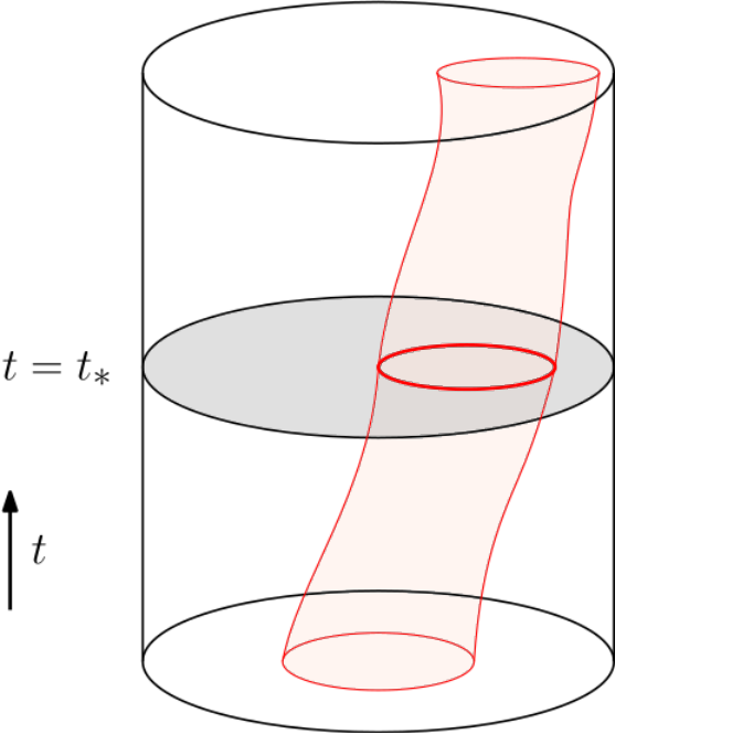
A notion of heating phase can be defined for general Virasoro processes. A general diffeomorphism corresponds to a probability distribution on the circle. Indeed it is positive and satisfies
| (5.38) |
The radius has a maximum at . This corresponds to a maximum of so we have . Hence the value of the radius there is
| (5.39) |
The heating phase corresponds to so that the black hole horizon approaches the boundary point . The heating phase then corresponds to
| (5.40) |
In the case where has a single maxima at going to infinity, we have
| (5.41) |
where is a smooth approximation of the delta function on the circle so that
| (5.42) |
The Möbius processes achieve this with the expression
| (5.43) |
where . This discussion mirrors the radial continuous majorization of the probability distributions (4.125) in Section 4.5.3. The holographic picture is then that the black hole horizon moves toward the point of the conformal boundary as depicted in Figure 14. We could also imagine more complicated limits where has multiple maxima going to infinity. In this case, the holographic picture involves a black hole horizon with a more complicated shape, approaching the boundary at various points.
The point of the circle to which the black hole tends becomes a heating point. Its antipode on the circle is a cooling point. We can define an effective temperature using the definition of the Virasoro state
| (5.44) |
so we have and the effective temperature is
| (5.45) |
where . In the heating phase, we see that there is a point on the circle at which the temperature becomes infinite. Note that the average temperature is conserved
| (5.46) |
So if a point becomes infinitely hot, the rest of the circle must cool down. This gives a holographic picture for the Floquet refrigerator Wen:2022pyj. The emergence of a hot spot and its holographic interpretation with a deforming black hole horizon was observed in the context of time evolution after a SSD quench in Goto:2021sqx.
6 Outlook and discussion
In this paper we have developed spacetime geometry and quantum information geometry of driven two-dimensional CFTs in the universal sector of Virasoro states. The BKM information geometry of Virasoro states gives new insight on complexity and ergodicity of driven CFTs. A particular truncation to the subgroup illuminates the rich dynamics of Möbius processes realized in Floquet CFTs. In this section we discuss some possible extensions for future work. It should be relatively straightforward to generalize our results to other subgroups generated by , and (see e.g. Liska:2022vrd) but we will leave this to future work.
Ergodic theory and Möbius driving.
As we have seen, the dynamics of a thermal CFT under Möbius driving reduces to measure-preserving dynamics of the two-dimensional hyperbolic disk, the BKM geometry of Möbius states. This makes contact with a much studied branch of ergodicity – dynamics in hyperbolic spaces (see for example McMullenLectures and references therein). In this work we have investigated only some particular models with some first observations about ergodic and non-ergodic regimes and potential measures of interest. We anticipate that there is much more to explore, with more general driving protocols and more details. For example, we did not investigate whether in the ergodic regime the dynamics may also be mixing. There are also many contexts leading to consider various driven CFTs, where to apply and possibly generalize our approach. For example, driven Tomonaga–Luttinger liquids motivate a compact boson CFT with driving through alternating the compactification radius Datta:2022fwd. See also other models discussed therein.
Modeling the dynamics of open systems.
As one application of BKM geometry, we considered work dissipation in slowly driven open CFTs in contact with a heat bath. The driving resulted from a classical background metric which produced a time-dependent Hamiltonian. The treatment of dissipation under slow driving was based on the general framework developed in scandi_thermodynamic_2019; abiuso_geometric_2020, applicable to any open quantum system whose Hamiltonian is time-dependent due to explicit time-dependence in its parameters (arising from driving by classical time-dependent background fields). A simple example is a two-level system coupled to a harmonic potential where the width of the potential well can be varied.
In this setting, the classical background field injects energy into the system since the Hamiltonian eigenvalues depend on time. This leads to changes in the energy level spacing that affects the internal energy. A simplification in these models is that they hide the detailed origin of this energy by taking a limit of the master equation. There is a clear classical to quantum boundary where the system under consideration is quantum while the background fields are treated classically. Hence the internal energy can grow without bounds (which is what happens in the heating phase for example), but in practice, such growth cannot continue forever. The limit of the master equation also hides the details of how the environment exchanges heat with the system and where the dissipated work is absorbed.
A complete description involves a composite system-environment Hilbert space with a unitary composite Hamiltonian time evolution, from which open-system dynamics is obtained by tracing out the environment. In the case of finite-dimensional systems, there is extensive literature on such models. It would be interesting to develop analogous detailed models of driven CFTs interacting with an environment. It would also be interesting to develop a holographic understanding of such open quantum systems. Such a holographic description will presumably require matter fields, as without matter fields we can only consider diffeomorphisms in AdS which necessarily leave e.g. the entropy invariant. To include matter fields and their backreaction will introduce many new conceptual and technical complications beyond the scope of the present paper. It may also be possible to model open systems in a more universal way incorporating changes in energies and entropy using singular diffeomorphisms representing shockwaves. Diffeomorphisms of the real line which change the temperature of the thermal states appear to be of this form when we embed the Poincaré patch in global AdS. It would be interesting to explore this possibility in more detail.
Physical interpretation of geodesics.
The geodesics in the information geometry give the shortest path from an initial state to a target space. From a geodesic one can compute a particular driving protocol, which minimizes dissipated work in a slowly driven open CFT. For unitary driving it suggests an optimal way to synthesize the target state (an optimal quantum circuit minimizing a thermodynamically motivated notion of circuit complexity).
Higher work moments.
In this paper, we only considered the expected amount of work , the integral of the expectation value where is the driving Hamiltonian. As a further step, one could consider integrals of higher moments of , in particular the variance of performed work
| (6.1) |
measuring the expected amount of cumulative work fluctuations during the driving protocol. In general, one can define full work statistics by the so called two-projective-measurement (TPM) scheme, where work is measured by two projective measurements before and after the driving protocol tasaki_jarzynski_2000; kurchan_quantum_2001; talkner_fluctuation_2007; talkner_fluctuation_2009. In this way one can define a moment generating function, and take derivatives to compute moments of the work distribution. However, only in discrete processes these moments agree with (6.1) (see Appendix of miller_work_2019).
Quantum information geometry can also be used to optimize work fluctuations miller_work_2019: there exists a metric whose geodesics minimize (6.1). In fact, the integrand of (6.1) is related to the variance of relative entropy de_boer_quantum_2021
| (6.2) |
when the process is a step-equilibration process scandi_quantum_2020. We define the variance metric as (which is well defined due to )
| (6.3) |
and by using results of Section 3.2, we observe that for a step-equilibration process (see also scandi_quantum_2020)
| (6.4) |
As a result, (6.4) has its minimum value along geodesics of . As with the relative entropy variance here, one could use other information quantities to define many different information metrics on the BKM geometry. We leave a more detailed analysis of higher moments to future work.
Other information metrics.
In this work, we focused on the BKM quantum information metric which is a metric on mixed states and which is given by the Hessian of the relative entropy. More generally, the Hessian of any information divergence produces a metric on mixed states whose form is fixed by the perturbative expansion of the divergence. The variance metric presented in the previous paragraph is an example of this (see petz_riemannian_1996 for more examples). If the information divergence is unitary invariant, the corresponding metric should be right-invariant when restricted to Virasoro states like the BKM metric. For metrics restricted to Möbius states that can be identified with points of the unit disk , this would translate to right-invariance under the action of . Because the hyperbolic metric is the unique -invariant metric on (up to a constant), all these metrics are expected to be hyperbolic, but have different curvature radii. This might have implications for Möbius driving. We leave a more detailed study of these metrics to future work.
Other information metrics can also be defined on the space of pure states, instead of mixed states, such as the Fubini–Study metric Erdmenger:2021wzc; erdmenger_complexity_2022. In this case, the relevant state space is a Virasoro orbit of some initial pure state (such as the vacuum state). The space of pure states cannot be endowed with the BKM metric directly, because the relative entropy is ill-defined for states that are not full rank. However, it might still be possible to define a BKM metric on the vacuum orbit by taking a double scaling limit, where the temperature of the thermal state is taken to zero while simultaneously scaling the metric appropriately. It would be interesting to investigate the Fubini–Study geometry of Möbius states in Möbius driven CFTs and its relationship to the limit of the BKM geometry.
Higher dimensions.
The results of this paper can be generalized by considering different groups beyond or Virasoro. For example, one could consider conformal processes where one drives a thermal state in a higher-dimensional CFT using their conformal groups. For holographic CFTs, this would correspond to driving the AdS-Schwarzschild black hole using a time-dependent conformal generator. It would be interesting to study the dynamics of such processes and their holographic dual description.
Acknowledgments
We thank Johanna Erdmenger, Marius Gerbershagen, Antti Kupiainen, Diego Liska, R. Loganayagam and Anna-Lena Weigel for useful discussions during the completion of this work. JdB is supported by the European Research Council under the European Unions Seventh Framework Programme (FP7/2007-2013), ERC Grant agreement ADG 834878. VG acknowledges the postdoctoral program at ICTS for funding support through the Department of Atomic Energy, Government of India, under project no. RTI4001. JK is supported by the Osk. Huttunen foundation and by the Magnus Ehrnrooth foundation. EKV’s research has been conducted within the framework of InstituteQ - the Finnish Quantum Institute.
Appendix A Virasoro trajectories and diffeomorphisms of the circle
In this Appendix, we review projective representations of which are representations of the Virasoro group: the central extension of the universal covering group . For other references on the topic with similar content, see fewster_quantum_2005; oblak_bms_2017; moosavi_inhomogeneous_2019.
A.1 Unitary representations of the Virasoro group
The group of orientation-preserving diffeomorphisms of the circle is defined as
| (A.1) |
whose group operations are composition and inversion of diffeomorphisms. The group manifold is not simply connected and hence globally different2525 25 The covering is infinite-to-one, because the fundamental group of is . from its universal cover which is given by
| (A.2) |
The tangent space of at the point is spanned by tangent vectors obtained as derivatives
| (A.3) |
with . In this appendix, we assume that is the identity and tangent vectors at the identity are denoted as
| (A.4) |
On the Hilbert space, a diffeomorphism is represented by unitary operators , and a tangent vector at the identity is represented by a Hermitian operator which is defined as the derivative of . Given a trajectory such that (A.4) holds, we get
| (A.5) |
The unitaries represent the group multiplication of projectively up to a phase (see oblak_bms_2017 for a review)
| (A.6) |
where the Thurston–Bott 2-cocycle
| (A.7) |
The projective multiplication law (A.6) is the group multiplication law of the Virasoro group which is the central extension of . Hence projective representations of correspond to ordinary representations of the Virasoro group.
In addition to the above representation, we can obtain an alternative one by taking the complex conjugate which satisfies
| (A.8) |
A.2 The Virasoro algebra and the stress tensor
The Lie algebra of can be identified with the algebra of real valued vector fields on via . The Lie bracket of two vector fields is the standard one
| (A.9) |
which differs from the Lie bracket of by a well-known minus sign modin_geometric_2019. This sign will not play a role for us and we will write all expressions in terms of (A.9).
The generators of are2626 26 More precisely, these are generators of the complexification .
| (A.10) |
and any vector field can be expanded in a Fourier series
| (A.11) |
For the generators, the bracket (A.9) is
| (A.12) |
On the Hilbert space, a vector field is represented by the Hermitian operator (A.5) which by linearity has the expansion
| (A.13) |
where we have defined with . The stress tensor is defined as
| (A.14) |
where the -periodic delta function
| (A.15) |
By linearity of the representation, it thus follows that
| (A.16) |
and (A.13) can also be written as
| (A.17) |
The operators satisfy the central extension of the algebra which is the Virasoro algebra.2727 27 More precisely, the Virasoro algebra is the central extension of . The Lie bracket between elements can be derived using (A.5) as follows.
Using (A.5), the adjoint action of a Virasoro unitary on an element of the Virasoro algebra is given by
| (A.18) |
By using the composition formula (A.6) of Virasoro unitaries and taking derivatives of the 2-cocycle (A.7), we get
| (A.19) |
where the adjoint action of on is given by
| (A.20) |
and the Schwarzian derivative is given by
| (A.21) |
Using (A.5), the commutator of two elements of the Virasoro algebra is obtained from the adjoint action as
| (A.22) |
Denoting , we have
| (A.23) |
so that
| (A.24) |
For the generators (A.10), this amounts to the standard form of the Virasoro algebra
| (A.25) |
where we used (A.12) in the first term. Similarly for the stress tensor (A.14), we get
| (A.26) |
The adjoint action (A.19) on the stress tensor (A.14) amounts to the standard transformation law
| (A.27) |
Complex conjugate representation.
The expressions for the complex conjugate represention of the Virasoro algebra is obtained by replacing in the above formulae. The stress tensor of the conjugate representation is
| (A.28) |
and algebra elements are . In a CFT, one forms a tensor product of the original and the complex conjugate representations. The conjugate representation is used for the quantization of the left-moving component of the two-dimensional stress tensor, namely, we have
| (A.29) |
as in (2.13). These conventions and signs match with moosavi_inhomogeneous_2019.
Virasoro Hamiltonian.
The Virasoro Hamiltonian is defined as
| (A.30) |
up to a constant which cancels in the definition of the Virasoro state . Combined with (A.20), we get the expression for the Virasoro Hamiltonian in the main text
| (A.31) |
where we used (A.20) and that . Notice that the equality is up to a constant involving the Schwarzian derivative which cancels in the definition of a Virasoro state.
A.3 Virasoro unitary as a time-ordered exponential
The unitary operator can be written as a time-ordered exponential
| (A.32) |
where is a Hermitian operator and time decreases from the left to the right. It follows that the generator is given by
| (A.33) |
where we used . Using the composition rule (A.6), computing the derivative with respect to and using (A.5) gives
| (A.34) |
where and it matches with formulae in Oblak:2017ect; erdmenger_complexity_2020. Hence the unitary (A.32) is explicitly
| (A.35) |
where the phase is given by
| (A.36) |
Denote for the diffeomorphism at and consider the straight line from the identity to whose tangent vector is independent of . In this case, the unitary (A.35) reduces to
| (A.37) |
where is the time-independent tangent vector and there is no more time-ordering. This is the formula presented in fewster_quantum_2005; fewster_probability_2019. The argument can also be reversed: each tangent vector at the identity defines a straight line such that (A.37) represents the diffeomorphism obtained as the solution of the equation with .
Lastly, for the complex conjugate representation , the expression is given by (A.35) by replacing and .
Appendix B Decomposition of the Polyakov action
In this Appendix, we will derive the decomposition of the Polyakov action when the metric is parametrized in terms of .
B.1 Necessary identities
We will first give an overview of identities. We consider Lorentzian cylinder with light-ray coordinates and a two-dimensional diffeomorphism and define
| (B.1) |
where the derivative
| (B.2) |
The ratios are known as Beltrami differentials and we have
| (B.3) |
Notice that (B.1) is equivalent to
| (B.4) |
These equations are first order differential equations that fix as non-local functionals of or . In particular, the last two equations in (B.4) are the Beltrami equations.
Using (B.4) one can show that
| (B.5) |
and similarly
| (B.6) |
Now a general two-dimensional metric can be written as
| (B.7) |
where we have defined the coordinate whose differentials are given by
| (B.8) |
Hence the Weyl factors are related as
| (B.9) |
It follows that derivatives with respect to are given by
| (B.10) |
These identities are sufficient to derive the decomposition of the Polyakov action.
B.2 Decomposition in the parametrization
We consider the Polyakov action is
| (B.11) |
with the metric (B.7) given by
| (B.12) |
Now the Polyakov action can be written as cappelli_stress_1989
| (B.13) |
where the Liouville action is given by
| (B.14) |
Here is the covariant derivative compatible with and is the corresponding Ricci scalar.
What remains is to decompose . In coordinates defined in (B.8), the metric takes the form
| (B.15) |
where the Weyl factor
| (B.16) |
Using again (B.13), the Polyakov action is simply the Liouville action in these coordinates:
| (B.17) |
Expanding the product and integrating the cross term by parts gives
| (B.18) |
where we also used that the integration measures are related as
| (B.19) |
By using (B.10) combined with the identities (B.5), we get
| (B.20) |
Substituting to (B.18), rearranging and integrating by parts the terms involving gives
| (B.21) | ||||
| (B.22) |
Hence we can write the full Polyakov action of the metric (B.7) as
| (B.23) |
where denotes the Liouville action (B.14) and
| (B.24) | |||
| (B.25) |
B.2.1 Including a background Weyl factor
We can also include a “background” in the Weyl factor which will not be subtracted away as in Section 2.3. In other words, we write the metric (B.7) as
| (B.26) |
where so that this time
| (B.27) |
includes an additional Weyl factor . To obtain , we have to simply replace
| (B.28) |
in equation (B.18) and compute each term again. The result of the calculation is the same as (B.20), but with replacements
| (B.29) |
where the covariant derivatives are defined as
| (B.30) |
We will now assume that the Weyl factors are of the form
| (B.31) |
that are independent of time . Taking this into account in (B.29), we can do the replacements to get that the Polyakov action of the metric (B.7) is given by
| (B.32) |
where is the Liouville action of in the background metric (B.27) and
| (B.33) |
By using the identity (B.5) and integrating by parts multiple times, we get
| (B.34) |
where the Schwarzians are given by
| (B.35) |
We note that in the derivation of (B.34) from (B.33), terms proportional to and appear that vanish by .
B.3 Decomposition in the parametrization
For completeness, we will also derive the decomposition of the Polyakov action in the parametrization written in Verlinde:1989hv; verlinde_conformal_1990; nguyen_holographic_2021. As far as we are aware, an explicit derivation is not available in the literature.
The idea is the same as above. We consider the Polyakov action (B.11) of the metric (B.7) given by
| (B.36) |
where should not be confused with (B.15) of the previous section. The Polyakov action decomposes as
| (B.37) |
In coordinates defined in (B.8), the metric in (B.36) takes the form
| (B.38) |
where the Weyl factor this time is
| (B.39) |
which should not be confused with (B.16) of the previous section. The remaining part of the Polyakov action is
| (B.40) |
where we used
| (B.41) |
Again by using (B.10) combined with the identities (B.6), we get
| (B.42) |
Substituting to (B.40) and integrating by parts the terms involving gives
| (B.43) |
Hence we can write the full Polyakov action of the metric (B.7) as
| (B.44) |
where
| (B.45) | |||
| (B.46) |
The term has previously appeared in Verlinde:1989hv; verlinde_conformal_1990; nguyen_holographic_2021 and is known as the QBK term quillen_determinants_1985; belavin_algebraic_1986.
B.3.1 Including a background Weyl factor
The background Weyl factor can also be included in the Beltrami parametrization which was done in lazzarini_integrating_1998. For completeness, we will explain how to get the result of lazzarini_integrating_1998 in the special case when the background Weyl factor is a sum of right- and left-moving terms (we have not been able to reproduce the general result).
We write the metric (B.7) as
| (B.47) |
where so that instead of (B.38) we now have
| (B.48) |
In equation (B.40), this amounts to the replacement
| (B.49) |
where is given by (B.39). The resulting formulae (B.42) are the same up to the replacement
| (B.50) |
where the covariant derivatives are defined as
| (B.51) |
Now considering the special case , we get that the Polyakov action of the metric (B.7) is given by
| (B.52) |
where is the Liouville action of in the background metric (B.48) and
| (B.53) | ||||
| (B.54) | ||||
| (B.55) |
which matches with lazzarini_integrating_1998.
Appendix C Non-negativity of relative entropy between Virasoro states
Relative entropy between two Virasoro states was computed in Section 3.1 with the result
| (C.1) |
where we have defined
| (C.2) |
To prove non-negativity, we employ the average lemma schwartz_projectively_1992; balog_coadjoint_1998 which is the inequality
| (C.3) |
with an equality if and only if . Using (C.3) in (C.1), we get the lower bound
| (C.4) |
By using
| (C.5) |
we get
| (C.6) |
where the last inequality follows from the unitarity bound2828 28 By equation (2.42), we have from which (C.7) follows assuming the theory admits only positive energy states .
| (C.7) |
Hence relative entropy on the circle is non-negative. For , we have an equality in (C.4) which implies that if and only if as required.
References
- (1) T. Kitagawa, E. Berg, M. Rudner and E. Demler, Topological characterization of periodically driven quantum systems, Physical Review B 82 (Dec., 2010) 235114.
- (2) D. V. Else, B. Bauer and C. Nayak, Floquet Time Crystals, Physical Review Letters 117 (Aug., 2016) 090402.
- (3) T. Mori, Floquet States in Open Quantum Systems, 2203.16358.
- (4) C. Jarzynski, Nonequilibrium Equality for Free Energy Differences, Physical Review Letters 78 (Apr., 1997) 2690–2693.
- (5) C. Jarzynski, Equilibrium free-energy differences from nonequilibrium measurements: A master-equation approach, Physical Review E 56 (Nov., 1997) 5018–5035.
- (6) G. E. Crooks, Entropy production fluctuation theorem and the nonequilibrium work relation for free energy differences, Physical Review E 60 (Sept., 1999) 2721–2726.
- (7) H. Tasaki, Jarzynski Relations for Quantum Systems and Some Applications, Sept., 2000.
- (8) J. Kurchan, A Quantum Fluctuation Theorem, cond-mat/0007360.
- (9) P. Salamon and R. S. Berry, Thermodynamic Length and Dissipated Availability, Physical Review Letters 51 (Sept., 1983) 1127–1130.
- (10) K. H. Hoffmann, B. Andresen and P. Salamon, Measures of dissipation, Physical Review A 39 (Apr., 1989) 3618–3621.
- (11) L. Diósi, K. Kulacsy, B. Lukács and A. Rácz, Thermodynamic length, time, speed, and optimum path to minimize entropy production, The Journal of Chemical Physics 105 (Dec., 1996) 11220–11225.
- (12) D. A. Sivak and G. E. Crooks, Thermodynamic Metrics and Optimal Paths, Physical Review Letters 108 (May, 2012) 190602.
- (13) S. Deffner and E. Lutz, Nonequilibrium Entropy Production for Open Quantum Systems, Physical Review Letters 107 (Sept., 2011) 140404.
- (14) P. R. Zulkowski, D. A. Sivak, G. E. Crooks and M. R. DeWeese, Geometry of thermodynamic control, Physical Review E 86 (Oct., 2012) 041148.
- (15) P. R. Zulkowski and M. R. DeWeese, Optimal protocols for slowly driven quantum systems, Physical Review E 92 (Sept., 2015) 032113.
- (16) M. Scandi and M. Perarnau-Llobet, Thermodynamic length in open quantum systems, Quantum 3 (Oct., 2019) 197, [1810.05583].
- (17) H. J. D. Miller, M. Scandi, J. Anders and M. Perarnau-Llobet, Work fluctuations in slow processes: Quantum signatures and optimal control, Physical Review Letters 123 (Dec., 2019) 230603, [1905.07328].
- (18) P. Abiuso, H. J. D. Miller, M. Perarnau-Llobet and M. Scandi, Geometric optimisation of quantum thermodynamic processes, Entropy 22 (Sept., 2020) 1076, [2008.13593].
- (19) F. Weinhold, Metric geometry of equilibrium thermodynamics, The Journal of Chemical Physics 63 (Sept., 1975) 2479–2483.
- (20) G. Ruppeiner, Thermodynamics: A Riemannian geometric model, Physical Review A 20 (Oct., 1979) 1608–1613.
- (21) C. R. Rao, Information and the Accuracy Attainable in the Estimation of Statistical Parameters, in Breakthroughs in Statistics: Foundations and Basic Theory (S. Kotz and N. L. Johnson, eds.), Springer Series in Statistics, pp. 235–247. Springer, New York, NY, 1992.
- (22) S. Kullback and R. A. Leibler, On Information and Sufficiency, The Annals of Mathematical Statistics 22 (1951) 79–86.
- (23) N. Čencov, Statistical Decision Rules and Optimal Inference, vol. 53 of Translations of Mathematical Monographs. American Mathematical Society, Apr., 2000.
- (24) L. L. Campbell, An extended Čencov characterization of the information metric, Proceedings of the American Mathematical Society 98 (1986) 135–141.
- (25) N. Ay, J. Jost, H. V. Lê and L. Schwachhöfer, Information geometry and sufficient statistics, Probability Theory and Related Fields 162 (June, 2015) 327–364, [1207.6736].
- (26) M. Bauer, M. Bruveris and P. W. Michor, Uniqueness of the Fisher-Rao metric on the space of smooth densities, Differential Geometry and its Applications 49 (Dec., 2016) 23–42, [1411.5577].
- (27) C. W. Helstrom, Quantum detection and estimation theory, Journal of Statistical Physics 1 (1969) 231–252.
- (28) R. Balian, Y. Alhassid and H. Reinhardt, Dissipation in many-body systems: A geometric approach based on information theory, Physics Reports 131 (Jan., 1986) 1–146.
- (29) S. L. Braunstein and C. M. Caves, Statistical distance and the geometry of quantum states, Physical Review Letters 72 (May, 1994) 3439–3443.
- (30) H. Hasegawa, Non-Commutative Extension of the Information Geometry, in Quantum Communications and Measurement (V. P. Belavkin, O. Hirota and R. L. Hudson, eds.), pp. 327–337. Springer US, Boston, MA, 1995.
- (31) A. Uhlmann, Density operators as an arena for differential geometry, Reports on Mathematical Physics 33 (Aug., 1993) 253–263.
- (32) A. Uhlmann, Geometric phases and related structures, Reports on Mathematical Physics 36 (Oct., 1995) 461–481.
- (33) D. Petz and C. Sudár, Geometries of quantum states, Journal of Mathematical Physics 37 (June, 1996) 2662–2673.
- (34) E. A. Morozova and N. N. Chentsov, Markov invariant geometry on manifolds of states, Journal of Soviet Mathematics 56 (Oct., 1991) 2648–2669.
- (35) D. Petz, Monotone metrics on matrix spaces, Linear Algebra and its Applications 244 (Sept., 1996) 81–96.
- (36) R. Kubo, Statistical-Mechanical Theory of Irreversible Processes. I. General Theory and Simple Applications to Magnetic and Conduction Problems, Journal of the Physical Society of Japan 12 (June, 1957) 570–586.
- (37) H. Mori, Transport, Collective Motion, and Brownian Motion, Progress of Theoretical Physics 33 (Mar., 1965) 423–455.
- (38) D. Petz and G. Toth, The Bogoliubov inner product in quantum statistics, Letters in Mathematical Physics 27 (Mar., 1993) 205–216.
- (39) R. S. Ingarden, Information geometry in functional spaces of classical and quantum finite statistical systems, International Journal of Engineering Science 19 (Jan., 1981) 1609–1633.
- (40) D. Petz and H. Hasegawa, On the Riemannian metric of -entropies of density matrices, Letters in Mathematical Physics 38 (Oct., 1996) 221–225.
- (41) A. Lesniewski and M. B. Ruskai, Monotone Riemannian Metrics and Relative Entropy on Non-Commutative Probability Spaces, Journal of Mathematical Physics 40 (Nov., 1999) 5702–5724, [math-ph/9808016].
- (42) N. Lashkari and M. Van Raamsdonk, Canonical Energy is Quantum Fisher Information, Journal of High Energy Physics 2016 (2016) 1–26, [1508.00897].
- (43) S. Banerjee, J. Erdmenger and D. Sarkar, Connecting Fisher information to bulk entanglement in holography, arXiv:1701.02319 [gr-qc, physics:hep-th, physics:quant-ph] (Jan., 2017) , [1701.02319].
- (44) G. Vitagliano, A. Riera and J. I. Latorre, Volume-law scaling for the entanglement entropy in spin-1/2 chains, New Journal of Physics 12 (nov, 2010) 113049.
- (45) H. Katsura, Sine-square deformation of solvable spin chains and conformal field theories, Journal of Physics A: Mathematical and Theoretical 45 (feb, 2012) 115003.
- (46) G. Ramí rez, J. Rodríguez-Laguna and G. Sierra, From conformal to volume law for the entanglement entropy in exponentially deformed critical spin 1/2 chains, Journal of Statistical Mechanics: Theory and Experiment 2014 (oct, 2014) P10004.
- (47) G. Ramírez, J. Rodríguez-Laguna and G. Sierra, Entanglement over the rainbow, J. Stat. Mech. 1506 (2015) P06002, [1503.02695].
- (48) N. Ishibashi and T. Tada, Infinite circumference limit of conformal field theory, J. Phys. A 48 (2015) 315402, [1504.00138].
- (49) N. Ishibashi and T. Tada, Dipolar quantization and the infinite circumference limit of two-dimensional conformal field theories, Int. J. Mod. Phys. A 31 (2016) 1650170, [1602.01190].
- (50) K. Okunishi, Sine-square deformation and Möbius quantization of 2D conformal field theory, PTEP 2016 (2016) 063A02, [1603.09543].
- (51) X. Wen, S. Ryu and A. W. W. Ludwig, Evolution operators in conformal field theories and conformal mappings: Entanglement Hamiltonian, the sine-square deformation, and others, Phys. Rev. B 93 (2016) 235119, [1604.01085].
- (52) J. Rodríguez-Laguna, J. Dubail, G. Ramírez, P. Calabrese and G. Sierra, More on the rainbow chain: entanglement, space-time geometry and thermal states, Journal of Physics A: Mathematical and Theoretical 50 (mar, 2017) 164001.
- (53) S. Tamura and H. Katsura, Zero-energy states in conformal field theory with sine-square deformation, PTEP 2017 (2017) 113A01, [1709.06238].
- (54) E. Tonni, J. Rodríguez-Laguna and G. Sierra, Entanglement hamiltonian and entanglement contour in inhomogeneous 1D critical systems, J. Stat. Mech. 1804 (2018) 043105, [1712.03557].
- (55) T. Tada, Conformal Quantum Mechanics and Sine-Square Deformation, PTEP 2018 (2018) 061B01, [1712.09823].
- (56) V. Alba, S. N. Santalla, P. Ruggiero, J. Rodriguez-Laguna, P. Calabrese and G. Sierra, Unusual area-law violation in random inhomogeneous systems, J. Stat. Mech. 1902 (2019) 023105, [1807.04179].
- (57) E. Langmann and P. Moosavi, Diffusive Heat Waves in Random Conformal Field Theory, Physical Review Letters 122 (Jan., 2019) 020201, [1807.10239].
- (58) M. Gluza, P. Moosavi and S. Sotiriadis, Breaking of Huygens–Fresnel principle in inhomogeneous Tomonaga–Luttinger liquids, J. Phys. A 55 (2022) 054002.
- (59) X. Wen and J.-Q. Wu, Quantum dynamics in sine-square deformed conformal field theory: Quench from uniform to nonuniform conformal field theory, Phys. Rev. B 97 (2018) 184309, [1802.07765].
- (60) I. MacCormack, A. Liu, M. Nozaki and S. Ryu, Holographic Duals of Inhomogeneous Systems: The Rainbow Chain and the Sine-Square Deformation Model, J. Phys. A 52 (2019) 505401, [1812.10023].
- (61) K. Goto, M. Nozaki, K. Tamaoka, M. T. Tan and S. Ryu, Non-Equilibrating a Black Hole with Inhomogeneous Quantum Quench, 2112.14388.
- (62) X. Wen and J.-Q. Wu, Floquet conformal field theory, 1805.00031.
- (63) B. Lapierre, K. Choo, C. Tauber, A. Tiwari, T. Neupert and R. Chitra, Emergent black hole dynamics in critical Floquet systems, Phys. Rev. Res. 2 (2020) 023085, [1909.08618].
- (64) H. Bernien, S. Schwartz, A. Keesling, H. Levine, A. Omran, H. Pichler et al., Probing many-body dynamics on a 51-atom quantum simulator, Nature 551 (Nov., 2017) 579–.
- (65) A. Keesling, A. Omran, H. Levine, H. Bernien, H. Pichler, S. Choi et al., Quantum Kibble–Zurek mechanism and critical dynamics on a programmable Rydberg simulator, Nature 568 (apr, 2019) 207–211.
- (66) V. Borish, O. Marković , J. Hines, S. Rajagopal and M. Schleier-Smith, Transverse-Field Ising Dynamics in a Rydberg-Dressed Atomic Gas, Physical Review Letters 124 (feb, 2020) .
- (67) K. Slagle, D. Aasen, H. Pichler, R. S. K. Mong, P. Fendley, X. Chen et al., Microscopic characterization of Ising conformal field theory in Rydberg chains, Phys. Rev. B 104 (Dec, 2021) 235109.
- (68) P. Caputa and J. M. Magan, Quantum Computation as Gravity, Physical Review Letters 122 (June, 2019) 231302.
- (69) J. Erdmenger, M. Flory, M. Gerbershagen, M. P. Heller and A.-L. Weigel, Exact Gravity Duals for Simple Quantum Circuits, SciPost Phys. 13 (2022) 061, [2112.12158].
- (70) J. Nulton, P. Salamon, B. Andresen and Q. Anmin, Quasistatic processes as step equilibrations, The Journal of Chemical Physics 83 (July, 1985) 334–338.
- (71) J. Anders and V. Giovannetti, Thermodynamics of discrete quantum processes, New Journal of Physics 15 (Mar., 2013) 033022.
- (72) B. Oblak, Berry Phases on Virasoro Orbits, JHEP 10 (2017) 114, [1703.06142].
- (73) A. Polyakov, Quantum geometry of bosonic strings, Physics Letters B 103 (1981) 207–210.
- (74) M. Knecht, S. Lazzarini and F. Thuillier, Shifting the Weyl anomaly to the chirally split diffeomorphism anomaly in two dimensions, Physics Letters B 251 (Nov., 1990) 279–283.
- (75) S. Lazzarini, Integrating the Chirally Split Diffeomorphism Anomaly on a Compact Riemann Surface, Physics Letters B 436 (Sept., 1998) 73–83, [hep-th/9807077].
- (76) H. L. Verlinde and E. P. Verlinde, Confomal Field Theory and Geometric Quantization, in Trieste School and Workshop on Superstrings, 10, 1989.
- (77) H. L. Verlinde, Conformal Field Theory, 2-D Quantum Gravity and Quantization of Teichmuller Space, Nucl. Phys. B 337 (1990) 652–680.
- (78) M. Mehboudi and H. J. D. Miller, Thermodynamic length and work optimization for Gaussian quantum states, Physical Review A 105 (June, 2022) 062434.
- (79) V. Arnold, Sur la géométrie différentielle des groupes de Lie de dimension infinie et ses applications à l’hydrodynamique des fluides parfaits, Annales de l’Institut Fourier 16 (1966) 319–361.
- (80) V. I. Arnol’d, Mathematical methods of classical mechanics, vol. 60. Springer Science & Business Media, 2013.
- (81) B. Khesin and G. Misiolek, Euler equations on homogeneous spaces and Virasoro orbits, Advances in Mathematics 176 (June, 2003) 116–144.
- (82) M. Flory and M. P. Heller, Conformal field theory complexity from Euler-Arnold equations, JHEP 12 (2020) 091, [2007.11555].
- (83) J. Erdmenger, M. Gerbershagen and A.-L. Weigel, Complexity measures from geometric actions on Virasoro and Kac-Moody orbits, Journal of High Energy Physics 2020 (Nov., 2020) 3, [2004.03619].
- (84) P. Basteiro, J. Erdmenger, P. Fries, F. Goth, I. Matthaiakakis and R. Meyer, Quantum complexity as hydrodynamics, Physical Review D 106 (Sept., 2022) 065016.
- (85) B. Oblak and G. Kozyreff, Berry Phases in the Reconstructed KdV Equation, Chaos 30 (2020) 113114, [2002.01780].
- (86) J. K. Hunter and R. Saxton, Dynamics of Director Fields, SIAM Journal on Applied Mathematics 51 (1991) 1498–1521.
- (87) B. Khesin and G. Misiolek, Euler equations on homogeneous spaces and Virasoro orbits, arXiv Mathematics e-prints (Oct., 2002) math/0210397, [math/0210397].
- (88) J. Lenells, The Hunter-Saxton equation describes the geodesic flow on a sphere, Journal of Geometry and Physics 57 (Sept., 2007) 2049–2064.
- (89) J. Lenells, The Hunter–Saxton equation: A geometric approach, SIAM J. Math. Analysis 40 (01, 2008) 266–277.
- (90) R. Fan, Y. Gu, A. Vishwanath and X. Wen, Emergent Spatial Structure and Entanglement Localization in Floquet Conformal Field Theory, Phys. Rev. X 10 (2020) 031036, [1908.05289].
- (91) X. Wen, R. Fan, A. Vishwanath and Y. Gu, Periodically, quasiperiodically, and randomly driven conformal field theories, Phys. Rev. Res. 3 (2021) 023044, [2006.10072].
- (92) X. Wen, Y. Gu, A. Vishwanath and R. Fan, Periodically, Quasi-periodically, and Randomly Driven Conformal Field Theories (II): Furstenberg’s Theorem and Exceptions to Heating Phases, SciPost Phys. 13 (2022) 082, [2109.10923].
- (93) B. Han and X. Wen, Classification of deformed Floquet conformal field theories, Phys. Rev. B 102 (2020) 205125, [2008.01123].
- (94) R. Fan, Y. Gu, A. Vishwanath and X. Wen, Floquet conformal field theories with generally deformed Hamiltonians, SciPost Phys. 10 (2021) 049, [2011.09491].
- (95) P. Moosavi, Inhomogeneous conformal field theory out of equilibrium, Annales Henri Poincaré (Dec., 2021) 1–40, [1912.04821].
- (96) D. Das, R. Ghosh and K. Sengupta, Conformal Floquet dynamics with a continuous drive protocol, JHEP 05 (2021) 172, [2101.04140].
- (97) B. Lapierre and P. Moosavi, Geometric approach to inhomogeneous Floquet systems, Physical Review B 103 (Jun, 2021) .
- (98) X. Wen, R. Fan and A. Vishwanath, Floquet’s Refrigerator: Conformal Cooling in Driven Quantum Critical Systems, 2211.00040.
- (99) K. Choo, B. Lapierre, C. Kuhlenkamp, A. Tiwari, T. Neupert and R. Chitra, Thermal and dissipative effects on the heating transition in a driven critical system, SciPost Phys. 13 (2022) 104, [2205.02869].
- (100) V. Reimer, K. G. L. Pedersen, N. Tanger, M. Pletyukhov and V. Gritsev, Nonadiabatic effects in periodically driven dissipative open quantum systems, Physical Review A 97 (Apr, 2018) .
- (101) J. Li, A. K. Harter, J. Liu, L. de Melo, Y. N. Joglekar and L. Luo, Observation of parity-time symmetry breaking transitions in a dissipative Floquet system of ultracold atoms, Nature Communications 10 (Feb, 2019) .
- (102) K. Viebahn, J. Minguzzi, K. Sandholzer, A.-S. Walter, M. Sajnani, F. Görg et al., Suppressing dissipation in a Floquet-Hubbard system, Physical Review X 11 (Mar, 2021) .
- (103) P. Caputa and I. MacCormack, Geometry and Complexity of Path Integrals in Inhomogeneous CFTs, JHEP 01 (2021) 027, [2004.04698].
- (104) P. Caputa and D. Ge, Entanglement and geometry from subalgebras of the Virasoro, 2211.03630.
- (105) S. Das, B. Ezhuthachan, A. Kundu, S. Porey, B. Roy and K. Sengupta, Brane Detectors of a Dynamical Phase Transition in a Driven CFT, 2212.04201.
- (106) R. Auzzi, S. Elitzur, S. B. Gudnason and E. Rabinovici, Time-dependent stabilization in AdS/CFT, Journal of High Energy Physics 2012 (Aug., 2012) 35, [1206.2902].
- (107) R. Auzzi, S. Elitzur, S. B. Gudnason and E. Rabinovici, On periodically driven AdS/CFT, Journal of High Energy Physics 2013 (Nov., 2013) 16, [1308.2132].
- (108) T. Faulkner, Bulk Emergence and the RG Flow of Entanglement Entropy, Journal of High Energy Physics 2015 (2015) , [1412.5648].
- (109) N. Lashkari, Modular Hamiltonian of Excited States in Conformal Field Theory, Physical Review Letters 117 (2016) , [1508.03506].
- (110) G. Sárosi and T. Ugajin, Relative entropy of excited states in two dimensional conformal field theories, Journal of High Energy Physics 2016 (2016) 114, [1603.03057].
- (111) G. Sárosi and T. Ugajin, Relative entropy of excited states in conformal field theories of arbitrary dimensions, Journal of High Energy Physics 2017 (2017) 60, [1611.02959].
- (112) T. Faulkner, F. M. Haehl, E. Hijano, O. Parrikar, C. Rabideau and M. Van Raamsdonk, Nonlinear Gravity from Entanglement in Conformal Field Theories, arXiv:1705.03026 [gr-qc, physics:hep-th] (2017) , [1705.03026].
- (113) A. May and E. Hijano, The holographic entropy zoo, Journal of High Energy Physics 2018 (Oct., 2018) 36, [1806.06077].
- (114) T. Ugajin, Perturbative expansions of Rényi relative divergences and holography, arXiv:1812.01135 [hep-th] (2018) , [1812.01135].
- (115) D. Liska, V. Gritsev, W. Vleeshouwers and J. Minář, Holographic Quantum Scars, 2212.05962.
- (116) J. Erdmenger, M. Gerbershagen, M. P. Heller and A.-L. Weigel, From Complexity Geometry to Holographic Spacetime, arXiv:2212.00043.
- (117) L. Kong and I. Runkel, Algebraic Structures in Euclidean and Minkowskian Two-Dimensional Conformal Field Theory, 0902.3829.
- (118) M. Schottenloher, A mathematical introduction to conformal field theory, vol. 759. Springer, 2008.
- (119) B. Oblak, BMS Particles in Three Dimensions, arXiv:1610.08526 [gr-qc, physics:hep-th, physics:math-ph] (2017) , [1610.08526].
- (120) K. Nguyen, Holographic boundary actions in AdS3/CFT2 revisited, Journal of High Energy Physics 2021 (Oct., 2021) 218, [2108.01095].
- (121) M. Besken, J. de Boer and G. Mathys, On Local and Integrated Stress-Tensor Commutators, arXiv:2012.15724 [hep-th] (Dec., 2020) , [2012.15724].
- (122) F. M. Ciaglia, F. Di Cosmo, F. Di Nocera and P. Vitale, Monotone metric tensors in Quantum Information Geometry, 2203.10857.
- (123) A. Müller-Hermes and D. Reeb, Monotonicity of the Quantum Relative Entropy Under Positive Maps, Annales Henri Poincaré 18 (May, 2017) 1777–1788, [1512.06117].
- (124) R. Schwartz, A projectively natural flow for circle diffeomorphisms, Inventiones mathematicae 110 (Dec., 1992) 627–647.
- (125) J. Balog, L. Fehér and L. Palla, Coadjoint orbits of the Virasoro algebra and the global Liouville equation, International Journal of Modern Physics A 13 (Jan., 1998) 315–362, [hep-th/9703045].
- (126) J. Cotler and K. Jensen, A theory of reparameterizations for AdS3 gravity, Journal of High Energy Physics 2019 (Feb., 2019) 79, [1808.03263].
- (127) V. Cavina, A. Mari and V. Giovannetti, Slow Dynamics and Thermodynamics of Open Quantum Systems, Physical Review Letters 119 (Aug., 2017) 050601.
- (128) R. Alicki, The quantum open system as a model of the heat engine, Journal of Physics A: Mathematical and General 12 (May, 1979) L103–L107.
- (129) S. Vinjanampathy and J. Anders, Quantum Thermodynamics, Contemporary Physics 57 (Oct., 2016) 545–579, [1508.06099].
- (130) M. A. Nielsen, A geometric approach to quantum circuit lower bounds, arXiv:quant-ph/0502070.
- (131) G. E. Crooks, Measuring thermodynamic length, Physical Review Letters 99 (Sept., 2007) 100602, [0706.0559].
- (132) K. Modin, Geometric Hydrodynamics: From Euler, to Poincaré, to Arnold, arXiv:1910.03301 [math-ph] (Oct., 2019) , [1910.03301].
- (133) B. Kolev, Local well-posedness of the EPDiff equation: A survey, Journal of Geometric Mechanics 9 (2017) 167–189, [1611.05034].
- (134) J. Escher and B. Kolev, Right-invariant Sobolev metrics of fractional order on the diffeomorphism group of the circle, Journal of Geometric Mechanics 6 (2014) 335–372, [1202.5122].
- (135) B. Khesin, J. Lenells, G. Misiolek and S. C. Preston, Geometry of diffeomorphism groups, complete integrability and optimal transport, arXiv:1105.0643 [math] (May, 2011) , [1105.0643].
- (136) C. J. Fewster and S. Hollands, Quantum Energy Inequalities in two-dimensional conformal field theory, Reviews in Mathematical Physics 17 (June, 2005) 577–612, [math-ph/0412028].
- (137) C. J. Fewster and S. Hollands, Probability distributions for the stress tensor in conformal field theories, Letters in Mathematical Physics 109 (Apr., 2019) 747–780, [1805.04281].
- (138) S. Hollands, Relative entropy for coherent states in chiral CFT, Letters in Mathematical Physics 110 (Apr., 2020) 713–733, [1903.07508].
- (139) L. Panebianco, A formula for the relative entropy in chiral CFT, Letters in Mathematical Physics 110 (Sept., 2020) 2363–2381, [1911.10136].
- (140) J. J. Bisognano and E. H. Wichmann, On the duality condition for quantum fields, Journal of Mathematical Physics 17 (Mar., 1976) 303–321.
- (141) J. Cardy and E. Tonni, Entanglement Hamiltonians in two-dimensional conformal field theory, J. Stat. Mech. 1612 (2016) 123103, [1608.01283].
- (142) C. Gross and I. Bloch, Quantum simulations with ultracold atoms in optical lattices, Science 357 (2017) 995–1001.
- (143) F. Schäfer, T. Fukuhara, S. Sugawa, Y. Takasu and Y. Takahashi, Tools for quantum simulation with ultracold atoms in optical lattices, Nature Reviews Physics 2 (jul, 2020) 411–425.
- (144) L. Jiang, T. Kitagawa, J. Alicea, A. R. Akhmerov, D. Pekker, G. Refael et al., Majorana fermions in equilibrium and in driven cold-atom quantum wires, Phys. Rev. Lett. 106 (Jun, 2011) 220402.
- (145) F. Harper and R. Roy, Floquet topological order in interacting systems of bosons and fermions, Phys. Rev. Lett. 118 (Mar, 2017) 115301.
- (146) L. D’Alessio and M. Rigol, Long-time behavior of isolated periodically driven interacting lattice systems, Phys. Rev. X 4 (Dec, 2014) 041048.
- (147) P. Ponte, Z. Papić, F. Huveneers and D. A. Abanin, Many-body localization in periodically driven systems, Phys. Rev. Lett. 114 (Apr, 2015) 140401.
- (148) D. A. Abanin, W. De Roeck and F. Huveneers, Exponentially slow heating in periodically driven many-body systems, Phys. Rev. Lett. 115 (Dec, 2015) 256803.
- (149) M. Sato, S. Takayoshi and T. Oka, Laser-Driven Multiferroics and Ultrafast Spin Current Generation, Phys. Rev. Lett. 117 (Sep, 2016) 147202.
- (150) F. Grossmann, T. Dittrich, P. Jung and P. Hänggi, Coherent destruction of tunneling, Phys. Rev. Lett. 67 (Jul, 1991) 516–519.
- (151) J. W. Anderson, Hyperbolic geometry; 2nd ed., .
- (152) B. Lapierre, K. Choo, A. Tiwari, C. Tauber, T. Neupert and R. Chitra, Fine structure of heating in a quasiperiodically driven critical quantum system, Phys. Rev. Res. 2 (2020) 033461.
- (153) M. Kohmoto, L. P. Kadanoff and C. Tang, Localization problem in one dimension: Mapping and escape, Phys. Rev. Lett. 50 (Jun, 1983) 1870–1872.
- (154) S. Ostlund, R. Pandit, D. Rand, H. J. Schellnhuber and E. D. Siggia, One-dimensional Schrödinger equation with an almost periodic potential, Phys. Rev. Lett. 50 (Jun, 1983) 1873–1876.
- (155) D. Damanik, A. Gorodetski and W. Yessen, The Fibonacci hamiltonian, Inventiones mathematicae 206 (2016) 629–692.
- (156) C. McCarthy, G. Nop, R. Rastegar and A. Roitershtein, Random walk on the Poincaré disk induced by a group of Möbius transformations, Markov processes and related fields 25 (2019) 915.
- (157) G. Rosenberger, All generating pairs of all two-generator Fuchsian groups, Archiv der Mathematik 46 (1986) 198–204.
- (158) J. Gilman, Two-generator discrete subgroups of PSL(2,R). Memoirs of the American Mathematical Society; no.561. American Mathematical Society, Providence, R.I, 1995.
- (159) H. Furstenberg, Noncommuting random products, Transactions of the American Mathematical Society 108 (1963) 377–428.
- (160) G. H. Hardy, J. E. Littlewood and G. Pólya, Inequalities. Cambridge University Press, Cambridge, 1988.
- (161) H. Joe, Majorization, Randomness and Dependence for Multivariate Distributions, The Annals of Probability 15 (1987) 1217 – 1225.
- (162) Z. V. Herstraeten, M. G. Jabbour and N. J. Cerf, Continuous majorization in quantum phase space, 2108.09167.
- (163) J. M. Maldacena, The Large N limit of superconformal field theories and supergravity, Adv. Theor. Math. Phys. 2 (1998) 231–252, [hep-th/9711200].
- (164) O. Aharony, S. S. Gubser, J. M. Maldacena, H. Ooguri and Y. Oz, Large N field theories, string theory and gravity, Phys. Rept. 323 (2000) 183–386, [hep-th/9905111].
- (165) M. Banados, C. Teitelboim and J. Zanelli, The Black hole in three-dimensional space-time, Phys. Rev. Lett. 69 (1992) 1849–1851, [hep-th/9204099].
- (166) M. Banados, Three-dimensional quantum geometry and black holes, arXiv:hep-th/9901148 (1999) 147–169, [hep-th/9901148].
- (167) S. Ryu and T. Takayanagi, Holographic derivation of entanglement entropy from AdS/CFT, Phys. Rev. Lett. 96 (2006) 181602, [hep-th/0603001].
- (168) S. Ryu and T. Takayanagi, Aspects of Holographic Entanglement Entropy, JHEP 08 (2006) 045, [hep-th/0605073].
- (169) T. Hartman, C. A. Keller and B. Stoica, Universal Spectrum of 2d Conformal Field Theory in the Large c Limit, Journal of High Energy Physics 2014 (Sept., 2014) 118, [1405.5137].
- (170) M. M. Roberts, Time evolution of entanglement entropy from a pulse, arXiv:1204.1982 [hep-th] (Apr., 2012) , [1204.1982].
- (171) N. Anand, H. Chen, A. L. Fitzpatrick, J. Kaplan and D. Li, An Exact Operator That Knows Its Location, arXiv:1708.04246 [hep-th] (Oct., 2017) , [1708.04246].
- (172) L. Susskind, Three Lectures on Complexity and Black Holes, SpringerBriefs in Physics, Springer, 10, 2018, 1810.11563, DOI.
- (173) C. McMullen, Ergodic theory, geometry and dynamics, Lecture notes for Math 275 (2020) .
- (174) S. Datta, B. Lapierre, P. Moosavi and A. Tiwari, Marginal quenches and drives in Tomonaga-Luttinger liquids, SciPost Phys. 14 (2023) 108, [2206.11287].
- (175) P. Talkner, E. Lutz and P. Hänggi, Fluctuation theorems: Work is not an observable, Physical Review E 75 (May, 2007) 050102.
- (176) P. Talkner, M. Campisi and P. Hänggi, Fluctuation theorems in driven open quantum systems, Journal of Statistical Mechanics: Theory and Experiment 2009 (Feb., 2009) P02025.
- (177) J. de Boer, V. Godet, J. Kastikainen and E. Keski-Vakkuri, Quantum hypothesis testing in many-body systems, SciPost Physics Core 4 (June, 2021) 019, [2007.11711].
- (178) M. Scandi, H. J. D. Miller, J. Anders and M. Perarnau-Llobet, Quantum work statistics close to equilibrium, Physical Review Research 2 (June, 2020) 023377.
- (179) A. Cappelli and A. Coste, On the stress tensor of conformal field theories in higher dimensions, Nuclear Physics B 314 (Mar., 1989) 707–740.
- (180) D. Quillen, Determinants of Cauchy-Riemann operators over a Riemann surface, Functional Analysis and Its Applications 19 (Jan., 1985) 31–34.
- (181) A. A. Belavin and V. G. Knizhnik, Algebraic geometry and the geometry of quantum strings, Physics Letters B 168 (Mar., 1986) 201–206.