Graph-based methods coupled with specific distributional distances for adversarial attack detection
Abstract
Artificial neural networks are prone to being fooled by carefully perturbed inputs which cause an egregious misclassification. These adversarial attacks have been the focus of extensive research. Likewise, there has been an abundance of research in ways to detect and defend against them. We introduce a novel approach of detection and interpretation of adversarial attacks from a graph perspective. For an input image, we compute an associated sparse graph using the layer-wise relevance propagation algorithm [Bach et al., 2015]. Specifically, we only keep edges of the neural network with the highest relevance values. Three quantities are then computed from the graph which are then compared against those computed from the training set. The result of the comparison is a classification of the image as benign or adversarial. To make the comparison, two classification methods are introduced: 1) an explicit formula based on Wasserstein distance applied to the degree of node and 2) a logistic regression. Both classification methods produce strong results which lead us to believe that a graph-based interpretation of adversarial attacks is valuable.
1 Introduction
Artificial neural networks (ANN) are known to be prone to misclassifying carefully perturbed inputs [Goodfellow et al., 2015]. These perturbed inputs, called adversarial, have been at the forefront of research in the machine learning community for the past decade. There is a lot of interest in creating new adversarial detection and defense methods, especially as this has consequence for a variety of real-world domains that rely on ANN for classification [Cireşan et al., 2012], [Finlayson et al., 2019], [Xu et al., 2020].
But among the known methods it is apparent that few of them, as diverse as they are, study adversarial attacks from a graph theory perspective. The objective of this paper is the exploration of adversarial attacks using graph-based methods. Indeed, the ANN structure can be described by a graph. In the most basic example, if one considers a standard feedforward ANN, then in a graphical representation, the neurons are associated to vertices/nodes and the weights between them are associated to edges. One may take this representation as inspiration for studying ANN from a graph perspective, although we stress that there is more than one way to obtain a graph from an ANN.
In [Hassabis et al., 2017], the authors provide a survey of the history of interactions between neuroscience and artificial intelligence and they note how much of the modern success in artificial intelligence can be traced to the understanding of or inspiration by biological systems. There is a line of research in neuroscience that studies the brain using elements of graph theory [Bullmore and Sporns, 2009], and this provides some motivation for the use of graph-theoretic approaches to studying ANN. This can be seen as part of a wider effort in research that seeks to improve artificial intelligence using bio-inspired ideas called neuromorphic computing. More examples from neuromorphic computing are [Yang et al., 2023a], [Yang et al., 2022a], [Yang et al., 2023b], [Yang et al., 2022b]. Bio-inspired methods seek to bring the benefits of low-power consumption and more efficient performance or reliability by comparison and inspiration from the human brain.
In this document, we study the detection of adversarial examples using graphs. Given an input to the neural network, we compute an associated sparse graph. From this graph, we then use a combination of three indices: the most relevant outermost edges, the degree of nodes, and an importance measure. These indices are then used to predict whether the input is adversarial. For this purpose, we test two very different approaches- a logistic regression and a statistical test based on the Wasserstein distance applied to the degree of nodes. Lastly, we interpret the relative strength of attacks through our graph-based approach. An advantage of the detection methods introduced is that they include a thresholding step which is non-differentiable, thereby precluding gradient masking [Papernot et al., 2017] and making it difficult to make adaptive attacks. As part of our studies we also provide benchmarks.
2 Background and related work
There have been some efforts in interpreting ANN in graph-theoretic ways. The authors of [Zambra et al., 2020] study the existence and properties of motifs, clusters of neurons in ANN which appear often. In [La Malfa et al., 2022], the authors interpret ANN as a graph and study how MNIST and CIFAR datasets exhibit different distributions under defined quantities (e.g. node input strength, neuron strength). In [Corneanu et al., 2019], a topological study of ANN is made via its functional graph, a graph obtained from correlations of neurons. Other work [Mocanu et al., 2016],[Liu et al., 2020],[Naitzat et al., 2022] apply a similar topological view to studying ANN. Despite relating graphs to ANN, none of these articles demonstrate how to use graphs to detect adversarial examples, nor do they provide statistics on detection. An interesting use of graphs occurs in [Cheng et al., 2021] where they are used to evaluate the robustness of an ANN, as opposed to adversarial detection. In [Ma et al., 2018] (“LID”), [Lee et al., 2018], [Harder et al., 2021], and [Feinman et al., 2017], logistic regression is used to classify an input as benign or adversarial based on certain features, none of which are graph related. The Local Intrinsic Dimensionality (LID) of a sample is introduced in [Michael, 2017] and is motivated by the growth of the volume of a ball as a function of radius and dimension. In [Michael, 2017], an analogy is made by replacing volume with a cumulative probability distribution. The premise of LID is that adversarial examples exhibit significantly greater LID scores than do benign examples. Given a sample input to a pretrained neural network, the LID method begins by computing the neural network’s activations. For each activation, an approximation to its LID score is made, and the result is given to a logistic classifier to determine if the sample input is benign or adversarial. Statistical approaches to adversarial detection can be found in [Drenkow et al., 2022] (“RSA”) and [Roth et al., 2019], also neither of which use graph methods. In Random Subspace Analysis (RSA) [Drenkow et al., 2022], projections are used to lower the dimensionality of the space of the pretrained neural network’s activations before classifying an input as benign or adversarial. For each layer of the pretrained neural network, a set of approximate projection matrices are created to project the dimension of each layer onto a much smaller space. Then, class protoypes are defined for each class by obtaining the average of each neuron’s activations. For a given input to the neural network that one wishes to classify as benign or adversarial, the following is done: for a given layer and for each projection matrix, compute the distance in projected space between the class prototype and the sample input’s activations; record the class that minimizes this difference and add it to a set. After applying this procedure for each layer, one obtains a set of sets where the first set is indexed by layer and the second is indexed by the projection matrix. From this set of sets, a type of voting procedure is done and if the result is less than a threshold, the sample input is labeled adversarial. Our methods extend and complement the previous methods by showing the power of graph theory perspectives applied to studying adversarial attacks, from either a logistic regression or a pure statistics perspective. We also compare our methods with LID and RSA.
3 Graph generation and quantities of interest
To compute the associated directed graph for a neural network and input pair, we use layer-wise relevance propagation [Bach et al., 2015], [Montavon et al., 2019]. This algorithm produces a saliency map, but its intermediate steps allows one to assign quantities to neurons which can be interpreted as an indicator of the influence that a neuron has on the output. We begin by providing a brief overview of layer-wise relevance propagation. Following the notation in [Montavon et al., 2019] for the LRP- rule, signals are propagated from the output layer towards the input layers. For a neuron in layer that is connected to neuron in layer , the propagated signal from to is defined to be
| (1) |
where is the relevance of neuron , is the activation of neuron in layer ; is the weight between neurons ; is a small parameter; and . The relevance of a neuron in layer is given by
| (2) |
Equations (1) and (2) are used together recursively. To start the algorithm, one assigns the relevance of the output neurons of the neural network to be equal to the neural network output. Upon completion of the algorithm, we rank the edge relevance scores in descending order and keep the top 1%. Our thresholding is inspired by [Bullmore and Sporns, 2009], [Sporns, 2013]. In these works, the authors only keep the strongest connections. The edges that are kept become the edges in our induced graph . One can compute various quantities from . One such quantity is given by
| (3) |
where is the set of nodes and is the distance between vertices . We note that the distance between adjacent nodes is given by (1) and the distance between any pair of nodes is given by the path that corresponds to the shortest sum of distances of adjacent nodes. An intuitive meaning of (3) is that more importance is given to a vertex that has many neighbors and short distances to them. This equation is inspired by closeness centrality [Bavelas, 1950] which is given by
| (4) |
A difference between (3) and (4) is that the former is monotone in the cardinality of . For bipartite graphs, or “stacks” of bipartite graphs (one can think of multi-layer perceptrons) a measure of closeness centrality tends to be not useful, hence the motivation for (3).
Another quantity of interest is the degree of a vertex, which is defined to be the difference between out degree and in degree:
| (5) |
Our last quantity of interest are the values of certain edges of . This allows us to incorporate some of ’s topology. The edges we use are those that correspond to the last two layers of the original neural network. We only use these edges because using all edges would require a data structure of size , where is the number of nodes in layer . Clearly, this requires an extensive amount of memory when is large. One can see that in general, when using graph data, it is preferable, at least from a memory standpoint, to use a quantity whose size is much smaller than , for instance a dataset whose size is , where is the set of nodes. In fact, our use of degree and node importance as computed for each node meets this constraint.
In [Guo et al., 2022], the neurons just before the softmax layer are studied, which has a similarity with our study of outermost edge relevance. In that article, the authors use the said neurons to compare robustness of non-human primate and human vision with regards to adversarial images. This lends a further (biological) motivation to our use of outermost edge relevance. Since we apply a threshold to the edges of , there are nodes of which are not adjacent to an edge. More generally, the edges among the set need not be the same, where represents a set of graphs induced from the same architecture. To enforce consistency of representation for the outermost edge relevances we create a weighted adjacency matrix of the same dimension as the adjacency matrix for nodes in the last two layers. The edge relevance values that are above the threshold are recorded as is and those below this percentile are set to 0. The matrix is then flattened into a vector. This flattened vector is our third quantity of interest, and its nonzero components are given by (1), assuming the component is greater than the threshold.
Lastly, we note that it would be very difficult to create an adaptive attack to counter the methodology proposed here since our detection methods involve graph thresholding, a non-differentiable operation.
| formula | name |
|---|---|
| outermost edge relevance | |
| node importance | |
| degree |
4 A statistical test based on Wasserstein distances
The Wasserstein-1 distance between two probability distributions and defined on a measurable metric space is given by
| (6) |
where is the set of all measures on whose marginal distributions are given by and . In the case when consists of one sample and consists of discrete samples , then
| (7) |
where is the distribution with support at . Wasserstein distances have been applied to machine learning in several ways. In [Cherian and Aeron, 2020], Wasserstein distances are used to compress data into a small dimensional subspace while maintaining a large distance from adversarial distributions. Other work [Wong et al., 2019] uses Wasserstein distances to create adversarial attacks.
Our goal in using Wasserstein distances is different than those in the examples mentioned. Our goal is to apply Wasserstein differences for benign and adversarial graph statistics in order to classify an input as benign or adversarial. The statistic we are concerned with is degree.
Let denote the empirical distribution of degree in the case when benign inputs are correctly classified as belonging to class . Similarly, let denote the empirical distribution that corresponds to perturbed inputs which the model incorrectly classifies as belonging to class , and whose unperturbed image is correctly classified. Note that since we are concerned with degree, the domain of the distribution function is a vector whose dimension is equal to the number of nodes in the induced graphs. If for some input, the model outputs class , we would like to know if the output was generated by a random variable with distribution or with distribution where the lack of a hat denotes the true distribution.As before, we first construct the graph for the sample and compute a sample degree vector, which we denote by the random variable . For a yet to be defined subset of nodes , we define the following Wasserstein Sums Ratio (WSR) quantity:
| (8) |
where the in refers to the empirical distribution for node , and similarly for . Equation (8) says that for each node that belongs to , we compute Wasserstein-1 distances node-wise from the sample to the empirical distributions and we sum over the node indices and compute the ratio. If the ratio is less than some threshold, we classify the input as benign, otherwise as adversarial. It may occur that the denominator of (8) is equal to 0, thus, in this case, a small term is added to the numerator and denominator. This can happen if the empirical distributions only have support at a point. Lastly, we note that we could have also computed the Wasserstein distance in , where is the number of nodes in . However, that is a more involved procedure. Using (7), we can write (8) as
| (9) |
where is a sample from and is a sample from , and is the number of samples in , respectively for . Lastly, we make the set as follows: we calculate
| (10) |
where has distribution and has distribution and is expected value. We then create the set
| (11) |
The set identifies nodes where the mean of the benign distribution is greater than the adversarial distribution for all classes. Should it happen that is empty for some (we have experienced this only for one combination of model and attack), one may create a placeholder version of it by setting each entry to a very large negative value (the large negative value has the effect of removing the index from consideration when making the set ). Algorithm 1 shows adversarial detection using WSR.
The way we construct has the tendency to pick nodes that generalize well across all classes at the expense of nodes that specialize. In an alternative algorithm, we propose to use the specialized nodes. For a given output that is classified as class , we use . This can result in a more accurate test using our approach, but at the expense of a little longer computation since there are more nodes to use for computations. The algorithm is shown in Algorithm 2.
5 Consistency
We would like to analyze under what conditions (8) is a faithful predictor. We treat the case of a finite-width ANN with sufficiently many neurons. A finite-width ANN has the property that the degree distribution has compact support, which implies that the Wasserstein distance between an empirical degree distribution and true distribution is bounded, and the Wasserstein distance is continuous with respect to . We begin our proof of consistency by showing that given a real-valued random variable ; an empirical distribution of some other real-valued random variable with true distribution ; a function (whose arguments are a random variable and a distribution) that is uniformly continuous in the second argument with respect to ; and bounded, that
| (12) |
as . To prove (12), it is sufficient to show that
| (13) |
Under identical and independently distributed (iid) assumptions, the Glivenko-Cantelli lemma states that . This combined with the uniform continuity of in the second argument with respect to proves (13). To prove (12), we let and . From (13) we have for all as . We may combine this with the boundedness assumption to use the Lebesgue dominated convergence theorem, resulting in almost surely.
We now begin to analyze (8), and we start by supposing that our random variable corresponds to the benign case. Let
| (14) | ||||
For additional simplicity, let us assume that quantities defined in (14) are iid over the index . The iid assumption implies that
and
for all . By equation (12), the results we obtain going forward will hold for the population distribution in high probability assuming our empirical distributions have enough samples. By the weak law of large numbers,
Similarly,
Then (8) is equal to
| (15) |
where and are . If we consider the case when is adversarial, we get a similar limit as in (5). Thus for consistency, we need the two limits to not be equal, thus we write
| (16) |
where we use to denote adversarial quantities. This is equivalent to . This is a realistic assumption for distributions with different means. A classification threshold, , is then picked such that
| (17) |
An interesting example of (16) is the case in which and and where all terms do not equal 1. In this instance, (8) in the benign case will be the inverse of that in the adversarial case. Furthermore, neither ratio will equal 1. This happens when adversarial distributions are simply shifts of benign distributions.
6 Experimental details
6.1 Datasets
We train our models on MNIST, CIFAR-10, and SVHN datasets. For each model we create adversarial examples using the Adversarial Robustness Toolbox [Nicolae et al., 2018]. For CIFAR-10 and SVHN, all images were enlarged to (224, 224, 3). Images are preprocessed using built-in Keras layers that handle input preprocessing.
6.2 Architectures
We experiment with five models, two of which are detailed in Tables 2-3 while the other three are VGG-19, InceptionResnetV2 and MobileNet. The last layers of VGG-19, InceptionResnetV2, and MobileNet are preloaded from Keras, and their last layers are replaced with three custom, fully-connected layers, with output sizes 4096, 1000, and 10, respectively, and trained with ImageNet weights. With respect to these three models, we only compute graph-based quantities from these layers to keep the run-time reasonable. For models 1 and 2, we use all layers.
6.3 Hyperparameters
The values of and in our implementation of LRP- are 2 and , respectively. In our implementation of RSA we use , and the layer used is the third from the output layer. For creating noisy samples in the algorithm in LID, we use Gaussian noise of zero mean and variance 0.05. Also in our implementation of LID, we only use the last 10 layers for computational ease.
6.4 Attacks
We consider the fast gradient sign method, [Goodfellow et al., 2015], projected gradient descent [Madry et al., 2018], untargeted Carlini-Wagner L2 [Carlini and Wagner, 2017], DeepFool [Moosavi-Dezfooli et al., 2016], Square [Andriushchenko et al., 2020], and Auto [Croce and Hein, 2020] attacks. Fast gradient sign method attacks are clipped when perturbations are outside a ball of radius 10% in the norm. Projected gradient descent attacks are crafted using the same norm but with up to a 5% perturbation; the number of iterations was 40 except for InceptionResnetV2, MobileNet, and VGG19, in which 10 were used. Square and Auto attacks have the same norm and perturbation as projected gradient descent attacks. Optimization is done using ADAM with learning rate 0.01. For each attack we generate 10,000 adversarially perturbed images from 10,000 original (test data) images. In creating training data for the detection methods we introduce, approximately 14,000 samples were used, and the methods are compared on approximately 6,000 samples. For RSA the numbers are approximately the same. For LID, we use approximately 6,000 training and test samples each, with the exception of models 1 and 2 in which we use approximately 7,000 training and 3,000 test samples as these models were simpler and thus enabled faster computations.
| layer type | output size | activation function |
|---|---|---|
| fully connected | 300 | reLu |
| fully connected | 200 | reLu |
| fully connected | 150 | reLu |
| fully connected | 150 | reLu |
| fully connected | 100 | sigmoid |
| fully connected | 10 | softmax |
| layer type | output size | activation function |
|---|---|---|
| conv | 3 filters, kernel size (4,4) | identity |
| maxpool | pool size=(2,2), strides=(2,2) | reLu |
| conv | 3 filters, kernel size (4,4) | identity |
| maxpool | pool size=(2,2), strides=(2,2) | reLu |
| fully connected | 100 | reLu |
| fully connected | 10 | softmax |
7 Results and Discussion
7.1 Comparison of logistic regression approaches
In Tables , ,and we report the specificity (percentage benign samples that are correctly detected) and sensitivity (percentage adversarial samples that are correctly detected). One can see that the various graph statistics considered here can be strong, sensitive, and specific predictors of adversarial attacks in the case of using logistic regression. Among Mobilenet, InceptionResnetV2 and VGG19, the three graph-based statistics perform more or less the same in their classification of samples as benign or adversarial and they generally perform well. For instance, when MobileNet is given SVHN data that is attacked by Square, the specificity and sensitivity are 99.66% and 99.04%, respectively. From the tables, we see that the worst performance tends to occur under Carlini-Wagner and Deepfool attacks. These two attacks are believed to be among the most difficult to detect, so our results are consistent with this assumption. In particular, when VGG19 is given SVHN data that is attacked by Carlini-Wagner, the results show that our logistic regression models are good at detecting benign samples, but mostly fail to catch the adversarial ones. To be more concrete, when considering degree, the specificity and sensitivity are 97.67% and 29.68%, respectively. For node importance, the values are 98.84% and 9.68%, respectively. When using outermost edge relevance, the corresponding values are 100% and 0%, meaning that our detector erroneously classifies all input as benign; apparently in this case, the differences between outermost edge relevances in the benign and adversarial cases are too similar.
Among Model 1 and 2, degree is a significantly better predictor than node importance and outermost edge relevance, while outermost edge relevance for Model 2 is a poor predictor across all attacks, being unable to detect adversarial images. This is because the outermost edge relevance for benign and adversarial samples are thresholded to 0. The largest relevances for Model 2 are found in layers closer to the input layer.
In comparison to LID, our results are superior across almost all model/attack combinations. The tables show that for LID, the accuracy averaged between benign and adversarial detection rates is around 50% which is much less than than what we achieve using our graph-based statistics. We note that [Drenkow et al., 2022] also reports similar numbers for implementation of LID, thereby concurring with our results.
Lastly, in Figure 1, we include sample data for the three graph statistics introduced in Section 3. Note that because there are thousands of nodes, we only choose one node to show.
| model | Attack | |||||||
| FGSM | PGD | CW2 | DF | Sq | AA | |||
| MobileNet | degree | 99.64/98.10 | 99.63/99.23 | 82.21/90.74 | 80.23/91.34 | 94.08/93.22 | 100/99.63 | |
| node importance | 99.52/99.35 | 99.46/100 | 64.50/99.43 | 66.78/93.91 | 91.86/93.39 | 99.89/100 | ||
| outermost edge relevance | 100/99.98 | 99.71/99.61 | 85.27/90.06 | 87.75/89.24 | 100/99.85 | 100/99.86 | ||
| LID | 23.49/85.93 | 12.01/97.90 | 22.30/79.84 | 35.59/68.10 | 24.47/98.60 | 7.02/87.35 | ||
| InceptionResNetV2 | degree | 100/99.95 | 100/99.92 | 84.05/94.31 | 73.88/86.22 | 96.18/98.50 | 99.66/100 | |
| node importance | 100/100 | 100/100 | 65.76/88.13 | 44.12/96.08 | 89.30/99.36 | 100/99.96 | ||
| outermost edge relevance | 99.96/99.70 | 100/99.70 | 80.36/78.76 | 80.96/74.43 | 99.21/96.59 | 100/99.78 | ||
| LID | 40.13/66.23 | 76.58/44.09 | 21.08/73.91 | 72.97/28.78 | 67.79/41.59 | 31.60/75.93 | ||
| VGG19 | degree | 100/99.86 | 99.92/99.73 | 99.77/04.20 | 97.55/99.08 | 98.98/98.21 | 99.16/100 | |
| node importance | 99.96/100 | 99.96/100 | 100/0.70 | 94.88/99.35 | 98.24/98.28 | 97.97/100 | ||
| outermost edge relevance | 99.73/99.72 | 99.96/99.96 | 100/0 | 99.66/96.82 | 99.66/97.21 | 100/99.92 | ||
| LID | 79.66/6.57 | 99.39/42.71 | 41.77/57.55 | 99.73/0.88 | 98.78/0.11 | 22.14/76.08 | ||
| model | Attack | |||||||
| FGSM | PGD | CW2 | DF | Sq | AA | |||
| MobileNet | degree | 100/100 | 100/99.77 | 77.25/91.87 | 55.44/92.96 | 99.66/99.04 | 100/100 | |
| node importance | 100/100 | 99.66/100 | 55.61/90.53 | 54.39/88.69 | 89.30/99.36 | 100/99.96 | ||
| outermost edge relevance | 100/99.79 | 100/99.85 | 99.59/76.24 | 79.85/74.90 | 99.21/96.96 | 100/99.81 | ||
| LID | 57.12/40.29 | 69.78/37.14 | 77.47/23.03 | 92.97/7.03 | 88.45/7.71 | 85.23/37.52 | ||
| InceptionResNetV2 | degree | 99.88/99.84 | 98.63/100 | 76.00/91.52 | 75.29/92.63 | 87.35/97.11 | 99.41/100 | |
| node importance | 100/100 | 100/99.96 | 45.68/93.81 | 89.52/94.36 | 89.52/94.36 | 100/100 | ||
| outermost edge relevance | 99.96/99.68 | 100/99.60 | 74.06/76.25 | 92.95/90.58 | 92.95/90.58 | 100/99.92 | ||
| LID | 92.14/4.10 | 69.78/37.14 | 77.17/23.02 | 53.32/48.55 | 29.87/59.27 | 10.75/61.80 | ||
| VGG19 | degree | 100/99.93 | 100/100 | 97.67/29.68 | 98.80/99.18 | 96.97/99.57 | 99.96/100 | |
| node importance | 100/99.94 | 100/99.96 | 98.84/9.68 | 99.34/99.39 | 98.64/99.73 | 100/100 | ||
| outermost edge relevance | 100/99.88 | 100/99.81 | 100/0 | 99.96/98.37 | 100/97.83 | 100/99.92 | ||
| LID | 67.79/40.38 | 2.26/85.83 | 42.24/47.81 | 4.14/92.37 | 7.01/98.72 | 6.47/29.00 | ||
| model | Attack | |||||||
| FGSM | PGD | CW2 | DF | Sq | AA | |||
| Model 2 | degree | 99.00/95.45 | 99.90/95.45 | 98.05/99.19 | 97.26/99.20 | 99.86/65.44 | 99.97/95.34 | |
| node importance | 84.80/24.54 | 92.79/12.46 | 52.75/62.37 | 34.22/73.53 | 97.71/5.53 | 94.50/8.04 | ||
| outermost edge relevance | 100/0 | 100/0 | 100/0 | 100/0 | 100/0 | 100/0 | ||
| LID | 81.94/13.43 | 88.19/10.41 | 74.90/21.72 | 71.79/22.27 | 52.77/50.96 | 16.10/87.53 | ||
| Model 1 | degree | 95.96/98.91 | 94.76/84.19 | 6.58/88.76 | 95.51/96.71 | 98.63/71.97 | 96.02/84.48 | |
| node importance | 81.67/96.19 | 96.09/54.83 | 0.14/99.70 | 88.14/96.57 | 100/2.09 | 93.87/60.39 | ||
| outermost edge relevance | 90.34/86.50 | 89.31/85.25 | 49.55/42.19 | 95.68/93.58 | 100/0 | 89.47/88.57 | ||
| LID | 50.60/49.75 | 72.07/25.38 | 47.20/55.53 | 71.79/22.27 | 52.77/50.96 | 26.71/72.12 | ||


7.2 Comparison of statistical approaches
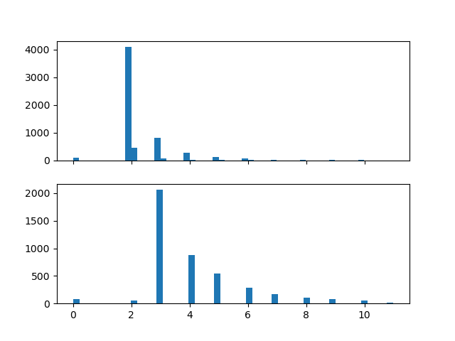
Tables , , and show results in terms of AUROC (area under receiver operating characteristic curve) for various detection methods. In almost all cases, WSR2 provides more accurate predictions than WSR1 as predicted in Section 5. Further, both WSR variations outperform RSA. Model 1, in comparison to the other models, performs somewhat poorly under WSR1. This seems to be due to Model 1 having the least number of neurons, making the corresponding relatively small which implies slower convergence of the statistical test. More generally, we can also see from the tables that model/attack pairs with small tend to have worse results under WSR. This is particularly noticeable in the case of Carlini-Wagner and Deepfool attacks under WSR1; this lower performance was also noted in our results using logistic regression, and provides evidence in support of the belief that Carlini-Wagner and Deepfool attacks are among the strongest. In Figure 2, one can see histograms of the distributions and for , . Because there are thousands of nodes, we only choose one value of to show.
| model | Attack | |||||||
| FGSM | PGD | CW2 | DF | Sq | AA | |||
| MobileNet | WSR1 | 99.98 | 100 | 79.78 | 73.56 | 92.98 | 100 | |
| WSR2 | 100 | 94.47 | 98.00 | 92.11 | 99.25 | 100 | ||
| RSA | 51.31 | 68.56 | 84.94 | 48.79 | 97.44 | 85.74 | ||
| InceptionResNetV2 | WSR1 | 99.64 | 99.00 | 81.46 | 64.23 | 84.88 | 100 | |
| WSR2 | 97.26 | 99.05 | 95.69 | 88.54 | 89.93 | 99.98 | ||
| RSA | 94.67 | 98.89 | 99.06 | 98.59 | 98.72 | 95.07 | ||
| VGG19 | WSR1 | 100 | 99.98 | 74.83 | 98.78 | 97.08 | 99.98 | |
| WSR2 | 99.87 | 99.97 | 97.36 | 99.32 | 99.70 | 100 | ||
| RSA | 69.08 | 54.28 | 71.70 | 73.77 | 76.58 | 63.78 | ||
| model | Attack | |||||||
| FGSM | PGD | CW2 | DF | Sq | AA | |||
| MobileNet | WSR1 | 100 | 100 | 81.62 | 78.95 | 99.29 | 100 | |
| WSR2 | 100 | 100 | 95.20 | 90.26 | 99.80 | 100 | ||
| RSA | 80.12 | 63.12 | 87.69 | 82.83 | 76.48 | 82.27 | ||
| InceptionResNetV2 | WSR1 | 100 | 100 | 78.35 | 80.59 | 92.12 | 100 | |
| WSR2 | 99.86 | 99.91 | 93.84 | 94.29 | 96.81 | 100 | ||
| RSA | 51.77 | 61.81 | 56.35 | 60.25 | 58.44 | 58.19 | ||
| VGG19 | WSR1 | 100 | 100 | 76.33 | 99.65 | 99.54 | 100 | |
| WSR2 | 100 | 100 | 94.57 | 99.68 | 99.87 | 100 | ||
| RSA | 80.69 | 57.27 | 76.79 | 79.63 | 81.77 | 58.23 | ||
| model | Attack | |||||||
| FGSM | PGD | CW2 | DF | Sq | AA | |||
| Model 2 | WSR1 | 95.16 | 95.37 | 96.48 | 95.44 | 91.77 | 95.54 | |
| WSR2 | 96.75 | 96.23 | 96.73 | 96.08 | 91.74 | 96.68 | ||
| RSA | 66.81 | 62.81 | 58.54 | 55.95 | 68.33 | 63.12 | ||
| Model 1 | WSR1 | 95.53 | 81.06 | 41.25 | 82.48 | 89.30 | 83.60 | |
| WSR2 | 96.36 | 94.40 | 39.65 | 97.81 | 99.48 | 94.36 | ||
| RSA | 71.80 | 72.10 | 51.64 | 89.60 | 96.34 | 71.85 | ||
![[Uncaptioned image]](2306.00042v2/class3_degree_node_426.png)


We can use WSR and logistic regression in a complementary way. For instance, graph-based quantities generated from VGG19 and Carlini-Wagner attacks tend to be poorly classified with logistic regression. In contrast, WSR2 performs well in this case, and it can be used in place of logistic regression.
As an aside, in [Roth et al., 2019], the authors claim that adding noise to images affects the logits in such a way that adversarial inputs can be detected. We considered using equation 5 from [Roth et al., 2019] as a baseline in place of RSA, but chose not to because of the extremely large time needed for the source code to run and secondly, our initial results suggested that this method gives poor accuracy, near 50%, which is much lower than the performance reports in the literature. In our effort to increase accuracy we experimented with different hyperparameters, including noise, but to no avail. This calls into question the usefulness and robustness of using equation 5 in [Roth et al., 2019].
7.3 Nodal analysis
The distribution of node quantities is highly dependent on the model and attack. It can be seen (Table 5) that AUROC for WSR decreases as the strength of the attack increases (we consider a partial order of in increasing attack strength to be: Fast Gradient Sign Method, Projected Gradient Descent and Carlini-Wagner L2). We can relate this observation to how the cardinality of varies with model/attack. The cardinality of can be seen in Tables , , and . For CIFAR-10 and SVHN datasets, we observe that the cardinality tends to be a lot smaller for Carlini-Wagner L2 and DeepFool attacks, and it seems to explain the lower accuracy achieved by WSR on these attacks. We recall that from Section 5, the accuracy of WSR increases with .
We also note that in some cases the benign distribution of WSR and the adversarial distribution of WSR are centered at points which are close to inverses. This seems to be the case for Model 2, as shown in Figure 3. This is in agreement with an earlier remark in Section 5 about equation (8) having inverse values under benign and adversarial examples.
| model | Attack | |||||||
| FGSM | PGD | CW2 | DF | Sq | AA | |||
| MobileNet | WSR1 | 877 | 734 | 51 | 68 | 405 | 79 | |
| InceptionResnetV2 | WSR1 | 378 | 484 | 109 | 180 | 240 | 120 | |
| VGG19 | WSR1 | 180 | 776 | 34 | 925 | 692 | 578 | |
| model | Attack | |||||||
| FGSM | PGD | CW2 | DF | Sq | AA | |||
| MobileNet | WSR1 | 422 | 636 | 78 | 97 | 551 | 287 | |
| InceptionResnetV2 | WSR1 | 754 | 1269 | 109 | 160 | 922 | 496 | |
| VGG19 | WSR1 | 945 | 1253 | 63 | 1379 | 929 | 843 | |
| model | Attack | |||||||
|---|---|---|---|---|---|---|---|---|
| FGSM | PGD | CW2 | DF | Sq | AA | |||
| Model 2 | WSR1 | 129 | 105 | 50 | 34 | 52 | 115 | |
| Model 1 | WSR1 | 33 | 10 | 7 | 5 | 4 | 10 | |
8 Conclusion
We demonstrate that neural network architectures can be interpreted in a graph context from which we can use the statistics of graph-based quantities to detect adversarial attacks. We introduce three statistics that we applied to our graphs and used them as predictors of adversarial attack. We show that this approach can produce high detection performances with logistic regression. We also study the distributions of node degree using a statistical test based on Wasserstein distances. One limitation of our method is that layer-wise relevance propagation is designed for ANNs with ReLU activations. Thus, the use of layer-wise relevance propagation may produce less explainability for neural networks with non-ReLu activations. However, ReLU is arguably the most popular type. It would be interesting to expand the class of neural networks in this study to include those with more non-ReLu activations, despite the possible gap in explainability. We note that Model 1 includes one non-ReLu activation (sigmoid) and it can be considered a small step in this direction. Another direction of our work may include the use of other saliency map methods such as [Springenberg et al., 2015] or [Simonyan et al., 2014] instead of layer-wise relevance propagation. Further, an ablation study can be done by removing specific and sensitive nodes from a neural network. In our context, these nodes can be from the set that is used in our statistical tests. It would be interesting to see the relationship between the neural network’s classification accuracy and the effectiveness of the statistical tests. We find it intriguing that a sparse graph encodes sufficient information about inputs to a neural network. We hope that the perspective introduced here will provide a different perspective of understanding adversarial attacks.
9 Acknowledgments
L. Carboni and D. Nwaigwe are the recipients of a grant from MIAI@Grenoble Alpes (ANR 19-P3IA-003).
References
- [Andriushchenko et al., 2020] Andriushchenko, M., Croce, F., Flammarion, N., and Hein, M. (2020). Square attack: A query-efficient black-box adversarial attack via random search. In Computer Vision - ECCV 2020 - 16th European Conference, Glasgow, UK, August 23-28, 2020, Proceedings, Part XXIII, volume 12368 of Lecture Notes in Computer Science, pages 484–501. Springer.
- [Bach et al., 2015] Bach, S., Binder, A., Montavon, G., Klauschen, F., Müller, K.-R., and Samek, W. (2015). On pixel-wise explanations for non-linear classifier decisions by layer-wise relevance propagation. PLOS ONE, 10(7):e0130140.
- [Bavelas, 1950] Bavelas, A. (1950). Communication patterns in task-oriented groups. The Journal of the Acoustical Society of America, 22(6):725–730.
- [Bullmore and Sporns, 2009] Bullmore, E. and Sporns, O. (2009). Complex brain networks: graph theoretical analysis of structural and functional systems. Nature Reviews Neuroscience, 10(3):186–198.
- [Carlini and Wagner, 2017] Carlini, N. and Wagner, D. (2017). Towards evaluating the robustness of neural networks. In 2017 IEEE Symposium on Security and Privacy (SP), pages 39–57, San Jose, CA, USA. IEEE.
- [Cheng et al., 2021] Cheng, W., Deng, C., Zhao, Z., Cai, Y., Zhang, Z., and Feng, Z. (2021). Spade: A spectral method for black-box adversarial robustness evaluation. In Proceedings of the 38th International Conference on Machine Learning, volume 139 of Proceedings of Machine Learning Research, pages 1814–1824. PMLR.
- [Cherian and Aeron, 2020] Cherian, A. and Aeron, S. (2020). Representation learning via adversarially-contrastive optimal transport. In Proceedings of the 37th International Conference on Machine Learning, Proceedings of Machine Learning Research. PMLR.
- [Cireşan et al., 2012] Cireşan, D., Meier, U., Masci, J., and Schmidhuber, J. (2012). Multi-column deep neural network for traffic sign classification. Neural Networks, 32:333–338.
- [Corneanu et al., 2019] Corneanu, C. A., Madadi, M., Escalera, S., and Martinez, A. M. (2019). What does it mean to learn in deep networks? And, how does one detect adversarial attacks? In 2019 IEEE/CVF Conference on Computer Vision and Pattern Recognition (CVPR), pages 4752–4761, Long Beach, CA, USA. IEEE.
- [Croce and Hein, 2020] Croce, F. and Hein, M. (2020). Reliable evaluation of adversarial robustness with an ensemble of diverse parameter-free attacks. In Proceedings of the 37th International Conference on Machine Learning, ICML 2020, 13-18 July 2020, Virtual Event, volume 119 of Proceedings of Machine Learning Research, pages 2206–2216. PMLR.
- [Drenkow et al., 2022] Drenkow, N., Fendley, N., and Burlina, P. (2022). Attack agnostic detection of adversarial examples via random subspace analysis. In 2022 IEEE/CVF Winter Conference on Applications of Computer Vision (WACV), pages 2815–2825, Waikoloa, HI, USA. IEEE.
- [Feinman et al., 2017] Feinman, R., Curtin, R. R., Shintre, S., and Gardner, A. B. (2017). Detecting adversarial samples from artifacts. arXiv preprint ARXIV.1703.00410.
- [Finlayson et al., 2019] Finlayson, S. G., Bowers, J. D., Ito, J., Zittrain, J. L., Beam, A. L., and Kohane, I. S. (2019). Adversarial attacks on medical machine learning. Science, 363(6433):1287–1289.
- [Goodfellow et al., 2015] Goodfellow, I. J., Shlens, J., and Szegedy, C. (2015). Explaining and harnessing adversarial examples. In 3rd International Conference on Learning Representations.
- [Guo et al., 2022] Guo, C., Lee, M., Leclerc, G., Dapello, J., Rao, Y., Madry, A., and Dicarlo, J. (2022). Adversarially trained neural representations are already as robust as biological neural representations. In Proceedings of the 39th International Conference on Machine Learning, volume 162 of Proceedings of Machine Learning Research, pages 8072–8081. PMLR.
- [Harder et al., 2021] Harder, P., Pfreundt, F.-J., Keuper, M., and Keuper, J. (2021). Spectraldefense: detecting adversarial attacks on cnns in the fourier domain. In 2021 International Joint Conference on Neural Networks (IJCNN), pages 1–8, Shenzhen, China. IEEE.
- [Hassabis et al., 2017] Hassabis, D., Kumaran, D., Summerfield, C., and Botvinick, M. (2017). Neuroscience-inspired artificial intelligence. Neuron, 95(2):245–258.
- [La Malfa et al., 2022] La Malfa, E., La Malfa, G., Caprioli, C., Nicosia, G., and Latora, V. (2022). Deep neural networks as complex networks. arXiv preprint ARXIV.2209.05488.
- [Lee et al., 2018] Lee, K., Lee, K., Lee, H., and Shin, J. (2018). A simple unified framework for detecting out-of-distribution samples and adversarial attacks. In Advances in Neural Information Processing Systems 31: Annual Conference on Neural Information Processing Systems, pages 7167–7177.
- [Liu et al., 2020] Liu, S., van der Lee, T., Yaman, A., Atashgahi, Z., Ferraro, D., Sokar, G., Pechenizkiy, M., and Mocanu, D. C. (2020). Topological insights into sparse neural networks. In Machine Learning and Knowledge Discovery in Databases - European Conference, ECML PKDD 2020, Ghent, Belgium, September 14-18, 2020, Proceedings, Part III, volume 12459 of Lecture Notes in Computer Science, pages 279–294. Springer.
- [Ma et al., 2018] Ma, X., Li, B., Wang, Y., Erfani, S. M., Wijewickrema, S. N. R., Schoenebeck, G., Song, D., Houle, M. E., and Bailey, J. (2018). Characterizing adversarial subspaces using local intrinsic dimensionality. In 6th International Conference on Learning Representations, ICLR 2018, Vancouver, BC, Canada, April 30 - May 3, 2018, Conference Track Proceedings. OpenReview.net.
- [Madry et al., 2018] Madry, A., Makelov, A., Schmidt, L., Tsipras, D., and Vladu, A. (2018). Towards deep learning models resistant to adversarial attacks. In International Conference on Learning Representations.
- [Michael, 2017] Michael, H. (2017). Local Intrinsic Dimensionality I: An Extreme-Value-Theoretic Foundation for Similarity Applications. In Similarity search and applications, SISAP, pages 64–79. Springer Berlin Heidelberg, New York, NY.
- [Mocanu et al., 2016] Mocanu, D. C., Mocanu, E., Nguyen, P. H., Gibescu, M., and Liotta, A. (2016). A topological insight into restricted Boltzmann machines. Machine Learning, 104(2-3):243–270.
- [Montavon et al., 2019] Montavon, G., Binder, A., Lapuschkin, S., Samek, W., and Müller, K.-R. (2019). Layer-Wise Relevance Propagation: An Overview, pages 193–209. Springer International Publishing, Cham.
- [Moosavi-Dezfooli et al., 2016] Moosavi-Dezfooli, S.-M., Fawzi, A., and Frossard, P. (2016). Deepfool: a simple and accurate method to fool deep neural networks. In 2016 IEEE Conference on Computer Vision and Pattern Recognition (CVPR), pages 2574–2582, Las Vegas, NV, USA. IEEE.
- [Naitzat et al., 2022] Naitzat, G., Zhitnikov, A., and Lim, L.-H. (2022). Topology of deep neural networks. Journal of Machine Learning Research, 21(1).
- [Nicolae et al., 2018] Nicolae, M.-I., Sinn, M., Tran, M. N., Buesser, B., Rawat, A., Wistuba, M., Zantedeschi, V., Baracaldo, N., Chen, B., Ludwig, H., Molloy, I., and Edwards, B. (2018). Adversarial robustness toolbox v1.2.0. CoRR, 1807.01069.
- [Papernot et al., 2017] Papernot, N., McDaniel, P., Goodfellow, I., Jha, S., Celik, Z. B., and Swami, A. (2017). Practical black-box attacks against machine learning. In Proceedings of the 2017 ACM on Asia Conference on Computer and Communications Security, pages 506–519, Abu Dhabi United Arab Emirates. ACM.
- [Roth et al., 2019] Roth, K., Kilcher, Y., and Hofmann, T. (2019). The odds are odd: A statistical test for detecting adversarial examples. In Proceedings of the 36th International Conference on Machine Learning, volume 97 of Proceedings of Machine Learning Research, pages 5498–5507. PMLR.
- [Simonyan et al., 2014] Simonyan, K., Vedaldi, A., and Zisserman, A. (2014). Deep inside convolutional networks: Visualising image classification models and saliency maps. In Bengio, Y. and LeCun, Y., editors, 2nd International Conference on Learning Representations, ICLR 2014, Banff, AB, Canada, April 14-16, 2014, Workshop Track Proceedings.
- [Sporns, 2013] Sporns, O. (2013). Structure and function of complex brain networks. Dialogues in Clinical Neuroscience, 15(3):247–262.
- [Springenberg et al., 2015] Springenberg, J. T., Dosovitskiy, A., Brox, T., and Riedmiller, M. A. (2015). Striving for simplicity: The all convolutional net. In 3rd International Conference on Learning Representations, ICLR 2015, San Diego, CA, USA, May 7-9, 2015, Workshop Track Proceedings.
- [Wong et al., 2019] Wong, E., Schmidt, F. R., and Kolter, J. Z. (2019). Wasserstein adversarial examples via projected sinkhorn iterations. In Proceedings of the 36th International Conference on Machine Learning, volume 97 of Proceedings of Machine Learning Research, pages 6808–6817. PMLR.
- [Xu et al., 2020] Xu, H., Ma, Y., Liu, H.-C., Deb, D., Liu, H., Tang, J.-L., and Jain, A. K. (2020). Adversarial attacks and defenses in images, graphs and text: a review. International Journal of Automation and Computing, 17(2):151–178.
- [Yang et al., 2023a] Yang, S., Pang, Y., Wang, H., Lei, T., Pan, J., Wang, J., and Jin, Y. (2023a). Spike-driven multi-scale learning with hybrid mechanisms of spiking dendrites. Neurocomputing, 542:126240.
- [Yang et al., 2022a] Yang, S., Tan, J., and Chen, B. (2022a). Robust spike-based continual meta-learning improved by restricted minimum error entropy criterion. Entropy, 24(4):455.
- [Yang et al., 2023b] Yang, S., Tan, J., Lei, T., and Linares-Barranco, B. (2023b). Smart traffic navigation system for fault-tolerant edge computing of internet of vehicle in intelligent transportation gateway. IEEE Transactions on Intelligent Transportation Systems, pages 1–12.
- [Yang et al., 2022b] Yang, S., Wang, J., Deng, B., Azghadi, M. R., and Linares-Barranco, B. (2022b). Neuromorphic context-dependent learning framework with fault-tolerant spike routing. IEEE Transactions on Neural Networks and Learning Systems, 33(12):7126–7140.
- [Zambra et al., 2020] Zambra, M., Maritan, A., and Testolin, A. (2020). Emergence of network motifs in deep neural networks. Entropy, 22(2):204.