Homogenization of nondivergence-form elliptic equations with discontinuous coefficients and finite element approximation of the homogenized problem

Timo Sprekeler Address: National University of Singapore, Department of Mathematics, 10 Lower Kent Ridge Road, Singapore 119076, Singapore. Email address: timo.sprekeler@nus.edu.sg

Date: August 11, 2026

Abstract.

We study the homogenization of the equation $-A(\frac{\cdot}{\varepsilon}):D^{2}u_{\varepsilon}=f$ posed in a bounded convex domain $\Omega\subset\mathbb{R}^{n}$ subject to a Dirichlet boundary condition and the numerical approximation of the corresponding homogenized problem, where the measurable, uniformly elliptic, periodic and symmetric diffusion matrix $A$ is merely assumed to be essentially bounded and (if $n>2$ ) to satisfy the Cordes condition. In the first part, we show existence and uniqueness of an invariant measure by reducing to a Lax–Milgram-type problem, we obtain $L^{2}$ -bounds for periodic problems in double-divergence-form, we prove homogenization under minimal regularity assumptions, and we generalize known corrector bounds and results on optimal convergence rates from the classical case of Hölder continuous coefficients to the present case. In the second part, we suggest and rigorously analyze an approximation scheme for the effective coefficient matrix and the solution to the homogenized problem based on a finite element method for the approximation of the invariant measure, and we demonstrate the performance of the scheme through numerical experiments.

Key words and phrases:

Homogenization, nondivergence-form elliptic PDE, Cordes condition, finite element methods

2010 Mathematics Subject Classification

35B27, 35J15, 65N12, 65N30

1. Introduction

In this paper, we discuss the homogenization of the linear elliptic nondivergence-form problem

(1.1)

\displaystyle\begin{split}-A\left(\frac{\cdot}{\varepsilon}\right):D^{2}u_{\varepsilon}&=f\quad\text{in }\Omega,\\ u_{\varepsilon}&=g\quad\text{on }\partial\Omega,\end{split}

where $\varepsilon>0$ is a small parameter, $\Omega\subset\mathbb{R}^{n}$ is a bounded convex domain, $f\in L^{2}(\Omega)$ , $g\in H^{2}(\Omega)$ , and $A\in L^{\infty}(\mathbb{R}^{n};\mathbb{R}^{n\times n}_{\mathrm{sym}})$ is $\mathbb{Z}^{n}$ -periodic, uniformly elliptic, and (if $n>2$ ) satisfies the Cordes condition (2.2) which dates back to [10]. In this setting, it is known that there exists a unique solution $u_{\varepsilon}\in H^{2}(\Omega)$ to (1.1); see [27, 29]. We study homogenization of the problem (1.1) as well as the numerical approximation of the corresponding homogenized problem.

The theory of periodic homogenization for (1.1) is classical and well-understood if $A$ is Hölder continuous and $f,g$ and $\partial\Omega$ are sufficiently regular. In this case, it is known that as $\varepsilon\searrow 0$ we have that $(u_{\varepsilon})_{\varepsilon>0}$ converges in a suitable sense to the solution of the homogenized problem, i.e., the linear elliptic constant-coefficient problem

(1.2)

\displaystyle\begin{split}-\bar{A}:D^{2}u&=f\quad\text{in }\Omega,\\ u&=g\quad\text{on }\partial\Omega,\end{split}

where the effective coefficient matrix $\bar{A}:=\int_{Y}rA$ is obtained by integrating $A$ against an invariant measure $r$ , defined as the solution to the periodic problem

(1.3)

\displaystyle-D^{2}:(rA)=0\quad\text{in }Y,\qquad r\text{ is $Y$-periodic},\qquad\int_{Y}r=1,

where $Y:=(0,1)^{n}$ ; see e.g., [4, 6, 11, 22]. Further, optimal convergence rates and corrector bounds in suitable norms are available in the literature; see e.g., [17, 20, 25, 28]. For recent developments in stochastic homogenization of nondivergence-form problems, we refer to [1, 2, 3, 18, 19] and the references therein. It seems that the case of measurable diffusion matrices that are merely essentially bounded has not been studied yet and our first goal of this paper is to generalize various qualitative and quantitative homogenization results to this setting.

Concerning the development of numerical methods to approximate the solution to (1.1), it is well-known that, for small positive $\varepsilon$ , standard finite element methods require a very fine mesh that resolves the oscillations of the coefficients to deliver accurate approximations. Therefore, multiscale finite element methods for nondivergence-form problems have been developed in recent years; see [9, 13] for linear problems and [16, 24] for Hamilton–Jacobi–Bellman (HJB) and Isaacs problems. For some results regarding finite difference schemes we refer to [8, 12, 14].

In particular, [13] suggests a multiscale finite element scheme based on the methodology of localized orthogonal decomposition (LOD) for linear nondivergence-form equations with essentially bounded measurable coefficients satisfying the Cordes condition. In [9], a multiscale finite element scheme for (1.1) with $A\in W^{1,q}_{\mathrm{per}}(Y;\mathbb{R}^{n\times n}_{\mathrm{sym}})$ , $q>n$ , and satisfying the Cordes condition has been suggested which is based on an approximation of the effective coefficient matrix via a finite element approximation of the invariant measure, relying on rewriting (1.3) in divergence-form. Since the latter is not possible in our setting, the second goal of this paper is to provide and analyze a finite element method for the approximation of the invariant measure in our case of merely essentially bounded measurable coefficients that satisfy the Cordes condition.

The structure of this paper is as follows.

In Section 2, we provide the framework, covering the main assumptions, well-posedness of (1.1), and a uniform $H^{2}$ -bound for the solution to (1.1). In Section 3, we study homogenization of (1.1). We begin by introducing a bilinear form, a coercivity property, and useful estimates that are used throughout the paper in Section 3.1. In Section 3.2, we analyze linear periodic problems in double-divergence-form and nondivergence-form. In particular, we find that any diffusion matrix $A$ that satisfies the assumptions stated below (1.1) has a unique invariant measure $r\in L^{2}_{\mathrm{per}}(Y)$ and that

(1.4)

\displaystyle r=C\frac{\mathrm{tr}(A)}{\lvert A\rvert^{2}}(1-\Delta\psi),

where $C$ is a positive constant and $\psi$ is the unique solution to a Lax–Milgram-type problem in the subspace of $H^{2}_{\mathrm{per}}(Y)$ consisting of functions with mean zero (see Theorem 3.1). In Section 3.3, we show that $(u_{\varepsilon})_{\varepsilon>0}$ converges weakly in $H^{2}(\Omega)$ to the unique solution $u\in H^{2}(\Omega)$ to the homogenized problem (1.2), using the transformation argument from [4]. Thereafter, in Sections 3.4 and 3.5, we obtain $H^{2}$ corrector estimates and generalize some results on type- $\varepsilon^{2}$ diffusion matrices (see Definition 3.3) obtained in [17] for Hölder continuous diffusion matrices to our setting.

In Section 4, we study the numerical approximation of the homogenized problem via a novel finite element method for the approximation of the invariant measure based on (1.4). We perform a rigorous error analysis and demonstrate the theoretical results in numerical experiments provided in Section 5. In Section 6, we collect the proofs of the results contained in this work.

2. Framework

Let $\Omega\subset\mathbb{R}^{n}$ be a bounded convex domain. Let $f\in L^{2}(\Omega)$ and $g\in H^{2}(\Omega)$ . For a small parameter $\varepsilon>0$ , we consider the problem

(2.1)

\displaystyle\begin{split}L_{\varepsilon}u_{\varepsilon}:=-A^{\varepsilon}:D^{2}u_{\varepsilon}&=f\quad\text{in }\Omega,\\ u_{\varepsilon}&=g\quad\text{on }\partial\Omega,\end{split}

where $A^{\varepsilon}:=A\left(\frac{\cdot}{\varepsilon}\right)$ and $A\in\mathcal{M}(\lambda,\Lambda)$ for some constants $\lambda,\Lambda>0$ . Here, we define

\displaystyle\mathcal{M}(\lambda,\Lambda):=\left\{A\in L^{\infty}(\mathbb{R}^{n};\mathbb{R}^{n\times n}_{\mathrm{sym}})\,\left\lvert A\text{ is $Y$-periodic and }\forall\xi\in\mathbb{R}^{n}\backslash\{0\}:\lambda\leq\frac{A\xi\cdot\xi}{\lvert\xi\rvert^{2}}\leq\Lambda\text{ a.e. in }\mathbb{R}^{n}\right.\right\},

where $Y:=(0,1)^{n}$ . We further assume that $A$ satisfies the Cordes condition (dating back to [10]), that is,

(2.2)

\displaystyle\exists\,\delta\in(0,1]:\qquad\frac{\lvert A\rvert^{2}}{(\mathrm{tr}(A))^{2}}\leq\frac{1}{n-1+\delta}\quad\text{a.e. in }\mathbb{R}^{n},

where $\lvert A\rvert:=\sqrt{A:A}$ . Note that this is no restriction for dimensions $n\leq 2$ :

Remark 2.1.

Let $A\in\mathcal{M}(\lambda,\Lambda)$ for some $\lambda,\Lambda>0$ . If $n\in\{1,2\}$ , the Cordes condition (2.2) holds:

(i)

If $n=1$ , we have that (2.2) holds with $\delta=1$ .
(ii)

If $n=2$ , we have that (2.2) holds with $\delta=\frac{\lambda}{\Lambda}$ . Indeed, this can be seen by writing $\lvert A\rvert^{2}$ as sum of the squared eigenvalues of $A$ and $\mathrm{tr}(A)$ as sum of the eigenvalues of $A$ , and using that $\frac{s^{2}+t^{2}}{(s+t)^{2}}\leq(1+\frac{s}{t})^{-1}$ for any $0<s\leq t$ .

The Cordes condition (2.2) guarantees the existence of a function $\gamma\in L^{\infty}_{\mathrm{per}}(Y)$ such that $\gamma>0$ and $\lvert\gamma A-I_{n}\rvert\leq\sqrt{1-\delta}$ almost everywhere, where $I_{n}$ denotes the identity matrix in $\mathbb{R}^{n\times n}$ .

Remark 2.2.

Let $A\in\mathcal{M}(\lambda,\Lambda)$ for some $\lambda,\Lambda>0$ and suppose that (2.2) holds. Then, the function

\displaystyle\gamma:=\frac{\mathrm{tr}(A)}{\lvert A\rvert^{2}}\in L^{\infty}(\mathbb{R}^{n})

is $Y$ -periodic, satisfies $\frac{\lambda}{\Lambda^{2}}\leq\gamma\leq\frac{\Lambda}{\lambda^{2}}$ almost everywhere, and there holds $\lvert\tilde{A}-I_{n}\rvert^{2}=n-\frac{(\mathrm{tr}(A))^{2}}{\lvert A\rvert^{2}}\leq 1-\delta$ almost everywhere, where $\tilde{A}:=\gamma A$ . Note that $\tilde{A}\in\mathcal{M}(\frac{\lambda^{2}}{\Lambda^{2}},\frac{\Lambda^{2}}{\lambda^{2}})$ .

It is then known (see [27, 29]) that (2.1) has a unique solution in $H^{2}(\Omega)$ . Further, we can obtain a uniform bound on the $H^{2}$ -norm of the solution.

Theorem 2.1 (well-posedness and uniform $H^{2}$ -bound).

Let $\Omega\subset\mathbb{R}^{n}$ be a bounded convex domain. Let $A\in\mathcal{M}(\lambda,\Lambda)$ , $f\in L^{2}(\Omega)$ , $g\in H^{2}(\Omega)$ , and suppose that (2.2) holds. Then, for any $\varepsilon>0$ there exists a unique solution $u_{\varepsilon}\in H^{2}(\Omega)$ to (2.1), and we have the bound

(2.3)

\displaystyle\|u_{\varepsilon}\|_{H^{2}(\Omega)}\leq C(\|f\|_{L^{2}(\Omega)}+\|g\|_{H^{2}(\Omega)})

for some constant $C=C(\mathrm{diam}(\Omega),\lambda,\Lambda,n,\delta)>0$ .

3. Homogenization

3.1. Preliminaries

Before we start with the main discussion we briefly highlight an important observation which will be crucial for this work. We write $L^{2}_{\mathrm{per},0}(Y):=\{\varphi\in L^{2}_{\mathrm{per}}(Y):\int_{Y}\varphi=0\}$ and $H^{k}_{\mathrm{per},0}(Y):=\{\varphi\in H^{k}_{\mathrm{per}}(Y):\int_{Y}\varphi=0\}$ for $k\in\mathbb{N}$ .

Lemma 3.1 (the bilinear form $b_{\mu}$ ).

\displaystyle b_{\mu}:H^{2}_{\mathrm{per}}(Y)\times H^{2}_{\mathrm{per}}(Y)\rightarrow\mathbb{R},\qquad b_{\mu}(\varphi_{1},\varphi_{2}):=(\mu\varphi_{1}-\gamma A:D^{2}\varphi_{1},\mu\varphi_{2}-\Delta\varphi_{2})_{L^{2}(Y)}

satisfies the bound

\displaystyle\mu^{2}\|\varphi\|_{L^{2}(Y)}^{2}+2\mu\|\nabla\varphi\|_{L^{2}(Y)}^{2}+\|D^{2}\varphi\|_{L^{2}(Y)}^{2}=\|\mu\varphi-\Delta\varphi\|_{L^{2}(Y)}^{2}\leq C_{\delta}\,b_{\mu}(\varphi,\varphi)\qquad\forall\varphi\in H^{2}_{\mathrm{per}}(Y),

where $C_{\delta}:=(1-\sqrt{1-\delta})^{-1}>0$ . In particular, if $\mu>0$ we have that $b_{\mu}$ is coercive on $H^{2}_{\mathrm{per}}(Y)$ , and if $\mu=0$ we have that $b_{\mu}$ is coercive on $H^{2}_{\mathrm{per},0}(Y)$ .

The following inequalities will be used frequently:

Remark 3.1.

For any $v\in H^{1}_{\mathrm{per},0}(Y)$ we have the Poincaré inequality $\|v\|_{L^{2}(Y)}\leq\frac{\sqrt{n}}{\pi}\|\nabla v\|_{L^{2}(Y)}$ ; see e.g., [5]. Further, for any $\varphi\in H^{2}_{\mathrm{per}}(Y)$ we have the identity $\|D^{2}\varphi\|_{L^{2}(Y)}=\|\Delta\varphi\|_{L^{2}(Y)}$ . In particular, there holds $\frac{\pi^{2}}{n}\|\varphi\|_{L^{2}(Y)}\leq\frac{\pi}{\sqrt{n}}\|\nabla\varphi\|_{L^{2}(Y)}\leq\|D^{2}\varphi\|_{L^{2}(Y)}=\|\Delta\varphi\|_{L^{2}(Y)}$ for any $\varphi\in H^{2}_{\mathrm{per},0}(Y)$ .

Using these results, we will now study periodic problems in double-divergence-form and nondivergence-form.

3.2. Periodic problems and invariant measures

In this section, we discuss the periodic double-divergence-form problem

(3.1)

\displaystyle-D^{2}:(qA)=f\quad\text{in }Y,\qquad q\text{ is Y-periodic},

and the periodic nondivergence-form problem

(3.2)

\displaystyle-A:D^{2}v=f\quad\text{in }Y,\qquad v\text{ is Y-periodic},

where $f\in L^{2}_{\mathrm{per}}(Y)$ , $A\in\mathcal{M}(\lambda,\Lambda)$ for some $\lambda,\Lambda>0$ , and we assume that the Cordes condition (2.2) holds. We seek solutions $q\in L^{2}_{\mathrm{per}}(Y)$ to (3.1), i.e., $(q,-A:D^{2}\varphi)_{L^{2}(Y)}=(f,\varphi)_{L^{2}(Y)}$ for any $\varphi\in H^{2}_{\mathrm{per}}(Y)$ . First, we introduce the notion of an invariant measure; see also [6, 7].

Definition 3.1 (invariant measure).

Let $A\in\mathcal{M}(\lambda,\Lambda)$ for some $\lambda,\Lambda>0$ . A function $r\in L^{2}_{\mathrm{per}}(Y)$ is called an invariant measure to $A$ if $\int_{Y}r=1$ and $(r,-A:D^{2}\varphi)_{L^{2}(Y)}=0$ for all $\varphi\in H^{2}_{\mathrm{per}}(Y)$ .

Our first result is the existence and uniqueness of an invariant measure $r\in L^{2}_{\mathrm{per}}(Y)$ to any $A\in\mathcal{M}(\lambda,\Lambda)$ satisfying the Cordes condition, and an $L^{2}$ -bound.

Theorem 3.1 (existence, uniqueness and properties of invariant measures).

Let $A\in\mathcal{M}(\lambda,\Lambda)$ for some $\lambda,\Lambda>0$ and suppose that (2.2) holds. Let $\gamma\in L^{\infty}_{\mathrm{per}}(Y)$ be defined as in Remark 2.2 and set $\tilde{A}:=\gamma A$ . Let $b_{0}:H^{2}_{\mathrm{per}}(Y)\times H^{2}_{\mathrm{per}}(Y)\rightarrow\mathbb{R}$ and $C_{\delta}>0$ be defined as in Lemma 3.1. Then, we have the following:

(i)

There exists a unique $\psi\in H^{2}_{\mathrm{per},0}(Y)$ such that $b_{0}(\varphi,\psi)=\int_{Y}\tilde{A}:D^{2}\varphi$ for any $\varphi\in H^{2}_{\mathrm{per},0}(Y)$ and we have the bound $\|\Delta\psi\|_{L^{2}(Y)}\leq\sqrt{n}\frac{\Lambda}{\lambda}C_{\delta}$ .
(ii)

The function $\tilde{r}:=1-\Delta\psi\in L^{2}_{\mathrm{per}}(Y)$ is the unique invariant measure to $\tilde{A}$ , and there holds $\tilde{r}\geq 0$ almost everywhere.

(iii)

The function $r:=(\gamma,\tilde{r})_{L^{2}(Y)}^{-1}\gamma\tilde{r}\in L^{2}_{\mathrm{per}}(Y)$ is the unique invariant measure to $A$ , and there holds $r\geq 0$ almost everywhere. Further, we have the bound

(3.3)

\displaystyle\|r\|_{L^{2}(Y)}\leq\frac{\Lambda^{3}}{\lambda^{3}}\|\tilde{r}\|_{L^{2}(Y)}\leq\frac{\Lambda^{3}}{\lambda^{3}}\left(\sqrt{n}\frac{\Lambda}{\lambda}C_{\delta}+1\right).

With Theorem 3.1 at hand, we can now state the main result on problems of the form (3.1).

Theorem 3.2 (analysis of the problem (3.1)).

Let $f\in L^{2}_{\mathrm{per}}(Y)$ , $A\in\mathcal{M}(\lambda,\Lambda)$ for some $\lambda,\Lambda>0$ , and suppose that (2.2) holds. Let $r\in L^{2}_{\mathrm{per}}(Y)$ denote the unique invariant measure to $A$ , and let $C_{\delta}>0$ be defined as in Lemma 3.1. Then, we have the following:

(i)

There exists a solution $q\in L^{2}_{\mathrm{per}}(Y)$ to the problem (3.1) if, and only if, $f\in L^{2}_{\mathrm{per},0}(Y)$ .
(ii)

If $f\in L^{2}_{\mathrm{per},0}(Y)$ and $q_{1},q_{2}\in L^{2}_{\mathrm{per}}(Y)$ are solutions to (3.1), then $q_{1}-q_{2}=cr$ with $c:=\int_{Y}(q_{1}-q_{2})$ . In particular, the problem (3.1) has a unique solution if $\int_{Y}q$ is prescribed.

(iii)

If $f\in L^{2}_{\mathrm{per},0}(Y)$ , then the unique solution $q_{0}\in L^{2}_{\mathrm{per},0}(Y)$ to (3.1) subject to $\int_{Y}q=0$ , whose existence and uniqueness follows from (i)-(ii), satisfies the bound

\displaystyle\|q_{0}\|_{L^{2}(Y)}\leq\frac{n\Lambda}{\pi^{2}\lambda^{2}}C_{\delta}\left(1+\|r\|_{L^{2}(Y)}\right)\|f\|_{L^{2}(Y)}.

Next, we turn to the analysis of the problem (3.2).

Theorem 3.3 (analysis of the problem (3.2)).

Let $f\in L^{2}_{\mathrm{per}}(Y)$ , $A\in\mathcal{M}(\lambda,\Lambda)$ for some $\lambda,\Lambda>0$ , and suppose that (2.2) holds. Let $\gamma\in L^{\infty}_{\mathrm{per}}(Y)$ be defined as in Remark 2.2 and let $b_{0}:H^{2}_{\mathrm{per}}(Y)\times H^{2}_{\mathrm{per}}(Y)\rightarrow\mathbb{R}$ and $C_{\delta}>0$ be defined as in Lemma 3.1. Let $r\in L^{2}_{\mathrm{per}}(Y)$ denote the unique invariant measure to $A$ . Then, we have the following:

(i)

There exists a solution $v\in H^{2}_{\mathrm{per}}(Y)$ to the problem (3.2) if, and only if, $(f,r)_{L^{2}(Y)}=0$ . Moreover, if $(f,r)_{L^{2}(Y)}=0$ , we have that $v\in H^{2}_{\mathrm{per}}(Y)$ is a solution to (3.2) if, and only if, $b_{0}(v,\varphi)=-(\gamma f,\Delta\varphi)_{L^{2}(Y)}$ for any $\varphi\in H^{2}_{\mathrm{per}}(Y)$ .
(ii)

If $(f,r)_{L^{2}(Y)}=0$ and $v_{1},v_{2}\in H^{2}_{\mathrm{per}}(Y)$ are solutions to (3.2), then $v_{1}-v_{2}=\mathrm{const.}$ almost everywhere. In particular, the problem (3.2) has a unique solution if $\int_{Y}v$ is prescribed.
(iii)

If $(f,r)_{L^{2}(Y)}=0$ , then the unique solution $v_{0}\in H^{2}_{\mathrm{per},0}(Y)$ to (3.2) subject to $\int_{Y}v_{0}=0$ , whose existence and uniqueness follows from (i)-(ii), satisfies the bound

$\displaystyle\|\Delta v_{0}\|_{L^{2}(Y)}\leq\frac{\Lambda}{\lambda^{2}}C_{\delta}\|f\|_{L^{2}(Y)}.$

We conclude this section by noting that the results regarding existence and uniqueness of solutions to (3.1) and (3.2) can also be obtained via the Fredholm alternative, observing that $K:L^{2}_{\mathrm{per}}(Y)\rightarrow L^{2}_{\mathrm{per}}(Y)$ , $f\mapsto(-\gamma A:D^{2}+\mu\,\mathrm{id})^{-1}f$ is a compact linear operator for $\mu>0$ due to Lemma 3.1. Our approach however is a constructive one and forms the basis for a simple construction of finite element methods for the numerical approximation of (3.1) and (3.2).

3.3. The convergence result

(3.4)

\displaystyle\begin{split}L_{\varepsilon}u_{\varepsilon}:=-A^{\varepsilon}:D^{2}u_{\varepsilon}&=f\quad\text{in }\Omega,\\ u_{\varepsilon}&=g\quad\text{on }\partial\Omega,\end{split}

where $\varepsilon>0$ is a small positive parameter. We recall from Theorem 2.1 that there exists a unique solution $u_{\varepsilon}\in H^{2}(\Omega)$ to (3.4) and that we have the uniform $H^{2}$ -bound (2.3). Thus, there exists a function $u\in H^{2}(\Omega)$ with $u-g\in H^{1}_{0}(\Omega)$ such that, upon passing to a subsequence,

(3.5)

\displaystyle u_{\varepsilon}\rightharpoonup u\quad\text{weakly in }H^{2}(\Omega)\text{ as }\varepsilon\searrow 0,\qquad u_{\varepsilon}\rightarrow u\quad\text{strongly in }H^{1}(\Omega)\text{ as }\varepsilon\searrow 0.

We denote the invariant measure to $A$ given by Theorem 3.1 by $r\in L^{2}_{\mathrm{per}}(Y)$ and multiply the equation $L_{\varepsilon}u_{\varepsilon}=f$ , which holds a.e. in $\Omega$ , by $r^{\varepsilon}:=r(\frac{\cdot}{\varepsilon})$ to obtain

(3.6)

\displaystyle-[rA]^{\varepsilon}:D^{2}u_{\varepsilon}=r^{\varepsilon}f\quad\text{a.e. in }\Omega,

where $[rA]^{\varepsilon}:=r^{\varepsilon}A^{\varepsilon}$ . Next, we apply the transformation argument from [4] (see also [23]) to obtain a divergence-form equation for $u_{\varepsilon}$ .

Noting that $rA\in L^{2}_{\mathrm{per}}(Y;\mathbb{R}^{n\times n}_{\mathrm{sym}})$ , we introduce $\phi_{j}\in H^{1}_{\mathrm{per},0}(Y)$ , $1\leq j\leq n$ , to be the unique solution in $H^{1}_{\mathrm{per},0}(Y)$ to the problem

(3.7)

\displaystyle-\Delta\phi_{j}=\nabla\cdot(rAe_{j})\quad\text{in }Y,\qquad\phi_{j}\text{ is $Y$-periodic},\qquad\int_{Y}\phi_{j}=0,

where $e_{j}\in\mathbb{R}^{n}$ denotes the $j$ -th column of $I_{n}$ . We set $\phi:=(\phi_{1},\dots,\phi_{n})\in H^{1}_{\mathrm{per},0}(Y;\mathbb{R}^{n})$ .

Remark 3.2.

We make the following observations:

(i)

For any $L\in\mathbb{N}$ and $1\leq j\leq n$ , the function $\phi_{j,L}:=\phi_{j}$ is the unique solution in $H^{1}_{\mathrm{per},0}(Y_{L})$ to

(3.8)

\displaystyle-\Delta\phi_{j,L}=\nabla\cdot(rAe_{j})\quad\text{in }Y_{L},\qquad\phi_{j,L}\text{ is $Y_{L}$-periodic},\qquad\int_{Y_{L}}\phi_{j,L}=0,

where $Y_{L}:=(0,L)^{n}$ . Indeed, note $\phi_{j,L}=\phi_{j,L}(\cdot+k)$ for any $k\in\mathbb{Z}^{n}$ by uniqueness of solutions to (3.8). Hence, $\phi_{j,L}\in H^{1}_{\mathrm{per},0}(Y)$ solves (3.7) and thus, $\phi_{j,L}=\phi_{j}$ .

(ii)

There holds $\nabla\cdot\phi=0$ almost everywhere. Indeed, this follows from $\nabla\cdot\phi\in L^{2}_{\mathrm{per},0}(Y)$ and

\displaystyle(\nabla\cdot\phi,\Delta\varphi)_{L^{2}(Y)}=\sum_{j=1}^{n}(\nabla\phi_{j},\nabla(\partial_{j}\varphi))_{L^{2}(Y)}=-\sum_{j=1}^{n}(rAe_{j},\nabla(\partial_{j}\varphi))_{L^{2}(Y)}=0

for any $\varphi\in H^{2}_{\mathrm{per}}(Y)$ , where we have used in the last step that $(r,-A:D^{2}\varphi)_{L^{2}(Y)}=0$ .

Next, we define the skew-symmetric matrix-valued map $B=(b_{ij})_{1\leq i,j\leq n}\in L^{2}_{\mathrm{per},0}(Y;\mathbb{R}^{n\times n})$ by $b_{ij}:=\partial_{i}\phi_{j}-\partial_{j}\phi_{i}$ for $1\leq i,j\leq n$ and we set

\displaystyle M:=rA+B\in L^{2}_{\mathrm{per}}(Y;\mathbb{R}^{n\times n}).

We observe that for any $L\in\mathbb{N}$ and $1\leq j\leq n$ , writing $Y_{L}:=(0,L)^{n}$ , we have that

\displaystyle-(Me_{j},\nabla\varphi)_{L^{2}(Y_{L})}=(\nabla\phi_{j}-Be_{j},\nabla\varphi)_{L^{2}(Y_{L})}=(\partial_{j}\phi,\nabla\varphi)_{L^{2}(Y_{L})}=(\nabla\cdot\phi,\partial_{j}\varphi)_{L^{2}(Y_{L})}=0

for any $\varphi\in H^{1}_{\mathrm{per}}(Y_{L})$ , where we have used Remark 3.2(i) in the first equality and Remark 3.2(ii) in the last equality. Hence, we have for any bounded domain $\omega\subset\mathbb{R}^{n}$ that

(3.9)

\displaystyle(Me_{j},\nabla w)_{L^{2}(\omega)}=0\qquad\forall 1\leq j\leq n\quad\forall w\in H^{1}_{0}(\omega).

Indeed, let $L\in\mathbb{N}$ such that $\omega\subset k_{L}+Y_{L}$ with $k_{L}:=-\frac{L}{2}(1,\dots,1)\in\mathbb{R}^{n}$ , extend $w\in H^{1}_{0}(\Omega)$ to a function $\tilde{w}\in H^{1}_{0}(k_{L}+Y_{L})$ by setting $\tilde{w}=0$ a.e. in $(k_{L}+Y_{L})\backslash\omega$ , and define $\varphi\in H^{1}_{\mathrm{per}}(Y_{L})$ to be the $Y_{L}$ -periodic extension of $\tilde{w}$ to see that $(Me_{j},\nabla w)_{L^{2}(\omega)}=(Me_{j},\nabla\tilde{w})_{L^{2}(k_{L}+Y_{L})}=(Me_{j},\nabla\varphi)_{L^{2}(Y_{L})}=0$ .

Writing $M^{\varepsilon}:=M(\frac{\cdot}{\varepsilon})$ , we then obtain that

(3.10)

\displaystyle(M^{\varepsilon}\nabla u_{\varepsilon},\nabla v)_{L^{2}(\Omega)}=(-M^{\varepsilon}:D^{2}u_{\varepsilon},v)_{L^{2}(\Omega)}=(r^{\varepsilon}f,v)_{L^{2}(\Omega)}\qquad\forall v\in C_{c}^{\infty}(\Omega),

where the first equality follows from (3.9) and the second equality follows from (3.6) and skew-symmetry of $B$ . Finally, noting that due to the fact that $r\in L^{2}_{\mathrm{per}}(Y)$ , $M\in L^{2}_{\mathrm{per}}(Y;\mathbb{R}^{n\times n})$ and $\int_{Y}B=0$ we have

(3.11)

\displaystyle M^{\varepsilon}

\displaystyle\rightharpoonup\int_{Y}M=\int_{Y}rA\;\text{ weakly in }L^{2}(\Omega;\mathbb{R}^{n\times n}),\;\;r^{\varepsilon}\rightharpoonup\int_{Y}r=1\;\text{ weakly in }L^{2}(\Omega)\;\text{ as }\varepsilon\searrow 0,

we can use (3.5) to pass to the limit $\varepsilon\searrow 0$ in (3.10) to obtain the following convergence result:

Theorem 3.4 (convergence result).

Let $\Omega\subset\mathbb{R}^{n}$ be a bounded convex domain, $A\in\mathcal{M}(\lambda,\Lambda)$ for some $\lambda,\Lambda>0$ , $f\in L^{2}(\Omega)$ , $g\in H^{2}(\Omega)$ , and suppose that (2.2) holds. Denoting the invariant measure to $A$ by $r\in L^{2}_{\mathrm{per}}(Y)$ , we introduce $\bar{A}:=\int_{Y}rA\in\mathbb{R}^{n\times n}_{\mathrm{sym}}$ . Then, there holds $\lambda\lvert\xi\rvert^{2}\leq\bar{A}\xi\cdot\xi\leq\Lambda\lvert\xi\rvert^{2}$ for all $\xi\in\mathbb{R}^{n}$ , and the sequence of solutions $(u_{\varepsilon})_{\varepsilon>0}\subset H^{2}(\Omega)$ to (3.4) converges weakly in $H^{2}(\Omega)$ to the unique solution $u\in H^{2}(\Omega)$ to the homogenized problem

(3.12)

\displaystyle\begin{split}\bar{L}u:=-\bar{A}:D^{2}u&=f\quad\text{in }\Omega,\\ u&=g\quad\text{on }\partial\Omega.\end{split}

We call the symmetric positive definite matrix $\bar{A}$ the effective coefficient matrix.

3.4. Corrector estimates

It is by now standard how to obtain corrector estimates to any order in the classical $A\in C^{0,\alpha}$ setting, introducing suitable interior and boundary correctors and assuming that $u$ is sufficiently regular; see e.g. [25, 28]. For $A\in L^{\infty}$ , using the uniform $H^{2}$ -bound from Theorem 2.1 and using Theorem 3.3, one obtains the following results by arguing along the lines of [28]. To simplify the statement of the results, we introduce the following notation:

Definition 3.2 (the notation $T(A,a)$ ).

Let $a\in L^{2}_{\mathrm{per}}(Y)$ , $A\in\mathcal{M}(\lambda,\Lambda)$ for some $\lambda,\Lambda>0$ , and suppose that $A$ satisfies (2.2). Let $r\in L^{2}_{\mathrm{per}}(Y)$ denote the invariant measure to $A$ . Then, we define $T(A,a):=w$ to be the unique element $w\in H^{2}_{\mathrm{per},0}(Y)$ satisfying $-A:D^{2}w=a-(a,r)_{L^{2}(Y)}$ .

Theorem 3.5 (an $\mathcal{O}(\varepsilon)$ corrector estimate in the $H^{2}$ -norm).

Suppose that we are in the situation of Theorem 3.4 and assume that $u\in H^{4}(\Omega)$ . Set $v_{ij}:=T(A,a_{ij})\in H^{2}_{\mathrm{per},0}(Y)$ for $1\leq i,j\leq n$ and set $V:=(v_{ij})_{1\leq i,j\leq n}$ . Writing $\varphi^{\varepsilon}:=\varphi(\frac{\cdot}{\varepsilon})$ for $\varphi\in\{V,\partial_{i}V\}$ , we define $\eta_{\varepsilon}:=V^{\varepsilon}:D^{2}u$ and

\displaystyle p_{ij,\varepsilon}:=2[\partial_{i}V]^{\varepsilon}:D^{2}(\partial_{j}u)+\varepsilon V^{\varepsilon}:D^{2}(\partial^{2}_{ij}u),\qquad P_{\varepsilon}:=(p_{ij,\varepsilon})_{1\leq i,j\leq n}.

Then, writing $C_{\delta}:=(1-\sqrt{1-\delta})^{-1}>0$ and assuming that

(3.13)

\displaystyle\eta_{\varepsilon}\in H^{2}(\Omega)\quad\text{and}\quad P_{\varepsilon}\in L^{2}(\Omega)\text{ with }\|P_{\varepsilon}\|_{L^{2}(\Omega)}=\mathcal{O}(1),

there exists a constant $c_{0}=c_{0}(\mathrm{diam}(\Omega),n)>0$ such that

(3.14)

\displaystyle\left\|u_{\varepsilon}-u-\varepsilon^{2}(\eta_{\varepsilon}+\theta_{\varepsilon})\right\|_{H^{2}(\Omega)}\leq\frac{\Lambda}{\lambda}C_{\delta}c_{0}\|P_{\varepsilon}\|_{L^{2}(\Omega)}\,\varepsilon=\mathcal{O}(\varepsilon),

where $\theta_{\varepsilon}\in H^{2}(\Omega)$ denotes the unique solution to $L_{\varepsilon}\theta_{\varepsilon}=0$ in $\Omega$ , $\theta_{\varepsilon}=-\eta_{\varepsilon}$ on $\partial\Omega$ .

Remark 3.3.

The proof of Theorem 3.5 shows that (3.14) holds with

\displaystyle c_{0}:=\sqrt{n}\,\sup_{v\in H^{2}(\Omega)\cap H^{1}_{0}(\Omega)\backslash\{0\}}\frac{\|v\|_{H^{2}(\Omega)}}{\|\Delta v\|_{L^{2}(\Omega)}}.

Remark 3.4.

If $n\leq 3$ , in view of the Sobolev embeddings, $u\in H^{4}(\Omega)$ is sufficient to guarantee that the assumption (3.13) in Theorem 3.5 is met.

Corollary 3.1 ( $L^{\infty}$ -rate in dimension $n\leq 3$ ).

Suppose that we are in the situation of Theorem 3.4 and $n\leq 3$ . Then, if $u\in H^{4}(\Omega)$ , we have that $\|u_{\varepsilon}-u\|_{L^{\infty}(\Omega)}=\mathcal{O}(\varepsilon)$ .

Note that the result of Corollary 3.1 follows directly from Theorem 3.5, Remark 3.4, the Sobolev embedding $H^{2}(\Omega)\hookrightarrow L^{\infty}(\Omega)$ , and the fact that by the maximum principle (see e.g., [26]) we have the bound $\|\theta_{\varepsilon}\|_{L^{\infty}(\Omega)}\leq\|V^{\varepsilon}:D^{2}u\|_{L^{\infty}(\Omega)}\leq\|V\|_{L^{\infty}(\mathbb{R}^{n})}\|D^{2}u\|_{L^{\infty}(\Omega)}$ in dimension $n\leq 3$ .

Similarly, we can obtain an $\mathcal{O}(\varepsilon^{2})$ corrector estimate in the $H^{2}(\Omega)$ -norm.

Theorem 3.6 (an $\mathcal{O}(\varepsilon^{2})$ corrector estimate in the $H^{2}$ -norm).

Suppose that we are in the situation of Theorem 3.5 and assume that $u\in H^{5}(\Omega)$ . Set $\chi_{jkl}:=T(A,Ae_{j}\cdot\nabla v_{kl})\in H^{2}_{\mathrm{per},0}(Y)$ for $1\leq j,k,l\leq n$ and set $X:=(\chi_{jkl})_{1\leq j,k,l\leq n}$ . Writing $\varphi^{\varepsilon}:=\varphi(\frac{\cdot}{\varepsilon})$ for $\varphi\in\{V,X,\partial_{i}X\}$ , we define $\tilde{\eta}_{\varepsilon}:=X^{\varepsilon}:D^{3}u$ and

\displaystyle q_{ij,\varepsilon}:=V^{\varepsilon}:D^{2}(\partial^{2}_{ij}u)+4[\partial_{i}X]^{\varepsilon}:D^{3}(\partial_{j}u)+2\varepsilon X^{\varepsilon}:D^{3}(\partial^{2}_{ij}u),\qquad Q_{\varepsilon}:=(q_{ij,\varepsilon})_{1\leq i,j\leq n}.

Then, writing $C_{\delta}:=(1-\sqrt{1-\delta})^{-1}$ and assuming that

(3.15)

\displaystyle\tilde{\eta}_{\varepsilon}\in H^{2}(\Omega)\quad\text{and}\quad Q_{\varepsilon}\in L^{2}(\Omega)\text{ with }\|Q_{\varepsilon}\|_{L^{2}(\Omega)}=\mathcal{O}(1),

we have the bound

(3.16)

\displaystyle\|u_{\varepsilon}-u+2\varepsilon z_{\varepsilon}-\varepsilon^{2}(\eta_{\varepsilon}+\theta_{\varepsilon})-2\varepsilon^{3}(\tilde{\eta}_{\varepsilon}+\tilde{\theta}_{\varepsilon})\|_{H^{2}(\Omega)}\leq\frac{\Lambda}{\lambda}C_{\delta}c_{0}\|Q_{\varepsilon}\|_{L^{2}(\Omega)}\,\varepsilon^{2}=\mathcal{O}(\varepsilon^{2}),

where $c_{0}>0$ is as in Remark 3.3 and $\tilde{\theta}_{\varepsilon},z_{\varepsilon}\in H^{2}(\Omega)$ denote the unique solutions to $L_{\varepsilon}\tilde{\theta}_{\varepsilon}=0$ in $\Omega$ , $\tilde{\theta}_{\varepsilon}=-\tilde{\eta}_{\varepsilon}$ on $\partial\Omega$ , and $L_{\varepsilon}z_{\varepsilon}=-\sum_{j,k,l=1}^{n}(Ae_{j}\cdot\nabla v_{kl},r)_{L^{2}(Y)}\partial^{3}_{jkl}u$ in $\Omega$ , $z_{\varepsilon}=0$ on $\partial\Omega$ , respectively.

Remark 3.5.

If $n\leq 3$ , in view of the Sobolev embeddings, $u\in H^{5}(\Omega)$ is sufficient to guarantee that the assumption (3.15) in Theorem 3.6 is met.

Corollary 3.2 ( $L^{\infty}$ -bound in dimension $n\leq 3$ ).

Suppose that we are in the situation of Theorem 3.4 and $n\leq 3$ . Then, if $u\in H^{5}(\Omega)$ , we have that

(3.17)

\displaystyle\|u_{\varepsilon}-u+2\varepsilon z_{\varepsilon}\|_{L^{\infty}(\Omega)}=\mathcal{O}(\varepsilon^{2}),

where $z_{\varepsilon}\in H^{2}(\Omega)$ is defined as in Theorem 3.6.

Similarly to Theorems 3.5 and 3.6, corrector estimates in the $H^{2}(\Omega)$ -norm can be obtained to any order, assuming that $u$ is sufficiently regular and constructing suitable corrector functions.

3.5. Type- $\varepsilon^{2}$ diffusion matrices

First, let us generalize the definition of type- $\varepsilon^{2}$ diffusion matrices from [17] given for $A\in C^{0,\alpha}$ to our present situation.

Definition 3.3 (type- $\varepsilon^{2}$ and type- $\varepsilon$ diffusion matrices).

Let $A\in\mathcal{M}(\lambda,\Lambda)$ for some $\lambda,\Lambda>0$ . We set $c_{j}^{kl}(A):=(Ae_{j}\cdot\nabla v_{kl},r)_{L^{2}(Y)}$ for $1\leq j,k,l\leq n$ , where $r\in L^{2}_{\mathrm{per}}(Y)$ denotes the invariant measure to $A$ and $v_{kl}:=T(A,a_{kl})\in H^{2}_{\mathrm{per},0}(Y)$ . We call $A$ a type- $\varepsilon^{2}$ diffusion matrix if $C_{jkl}(A):=c_{j}^{kl}(A)+c_{k}^{jl}(A)+c_{l}^{jk}(A)=0$ for all $1\leq j,k,l\leq n$ . Otherwise, we call $A$ a type- $\varepsilon$ diffusion matrix.

Note that the function $z_{\varepsilon}$ in (3.16) and (3.17) vanishes for any $u\in H^{5}(\Omega)$ if and only if the symmetric part of the third-order homogenized tensor $(c_{j}^{kl})_{1\leq j,k,l\leq n}$ vanishes, or equivalently, if and only if $A$ is type- $\varepsilon^{2}$ . In particular, in the situation of Corollary 3.2, if $A$ is type- $\varepsilon^{2}$ we have that $\|u_{\varepsilon}-u\|_{L^{\infty}(\Omega)}=\mathcal{O}(\varepsilon^{2})$ whereas if $A$ is type- $\varepsilon$ we only have that $\|u_{\varepsilon}-u\|_{L^{\infty}(\Omega)}=\mathcal{O}(\varepsilon)$ and this rate $\mathcal{O}(\varepsilon)$ is optimal in general.

We can now extend the main results from [17] obtained for $A\in C^{0,\alpha}$ to our present case. The following results can then be proved by using arguments almost identical to [17].

Theorem 3.7 (diffusion matrices $A=C+aM$ are type- $\varepsilon^{2}$ ).

Let $C,M\in\mathbb{R}^{n\times n}_{\mathrm{sym}}$ , let $a\in L^{\infty}_{\mathrm{per}}(Y)$ , and suppose that $A:=C+aM$ is such that $A\in\mathcal{M}(\lambda,\Lambda)$ for some $\lambda,\Lambda>0$ and (2.2) holds. Set $w:=T(A,a)\in H^{2}_{\mathrm{per},0}(Y)$ and $v_{ij}:=T(A,a_{ij})\in H^{2}_{\mathrm{per},0}(Y)$ for $1\leq i,j\leq n$ . Then, we have the following results:

(i)

The invariant measure to $A$ is given by $r=1+M:D^{2}w$ .
(ii)

We have that $V:=(v_{ij})_{1\leq i,j\leq n}$ is given by $V=wM$ .
(iii)

There holds $-C:D^{2}w=ra-\bar{a}$ where $\bar{a}:=(a,r)_{L^{2}(Y)}$ .
(iv)

The third-order homogenized tensor vanishes, i.e., $c_{j}^{kl}(A)=0$ for all $1\leq j,k,l\leq n$ .

In particular, $A$ is a type- $\varepsilon^{2}$ diffusion matrix.

Theorem 3.8 (characterization of type- $\varepsilon^{2}$ diagonal diffusion matrices for $n=2$ ).

Let $A\in\mathcal{M}(\lambda,\Lambda)$ for $n=2$ and some $\lambda,\Lambda>0$ , and suppose that $\frac{1}{a}A=I_{2}+bM=:B$ for some $b\in L^{\infty}_{\mathrm{per}}(Y)$ , where $a:=\frac{1}{2}\mathrm{tr}(A)$ and $M:=\mathrm{diag}(1,-1)$ . Set $w_{A}:=T(A,a)\in H^{2}_{\mathrm{per},0}(Y)$ , $w_{B}:=T(B,b)\in H^{2}_{\mathrm{per},0}(Y)$ , and $v_{ij}:=T(A,a_{ij})\in H^{2}_{\mathrm{per},0}(Y)$ for $1\leq i,j\leq n$ . Then, we have the following results:

(i)

The invariant measure $r_{B}$ to $B$ is given by $r_{B}=1+M:D^{2}w_{B}$ , and the invariant measure $r_{A}$ to $A$ is given by $r_{A}=\frac{\bar{a}}{a}r_{B}$ where $\bar{a}:=(\frac{1}{a},r_{B})_{L^{2}(Y)}^{-1}=(a,r_{A})_{L^{2}(Y)}$ .
(ii)

We have that $V:=(v_{ij})_{1\leq i,j\leq n}$ is given by $V=w_{A}(I_{2}+\bar{b}M)+w_{B}M$ where $\bar{b}:=(b,r_{B})_{L^{2}(Y)}$ .
(iii)

There holds $-\Delta w_{B}=r_{B}b-\bar{b}$ .
(iv)

There holds $c^{kl}_{3-s}(A)=2(-1)^{s+1}\bar{a}(1+m_{kl}\bar{b})(\partial_{3-s}w_{A},\partial^{2}_{ss}w_{B})_{L^{2}(Y)}$ for any $s,k,l\in\{1,2\}$ .

In particular, $A$ is type- $\varepsilon^{2}$ if, and only if, $(\partial_{1}w_{A},\partial^{2}_{22}w_{B})_{L^{2}(Y)}=(\partial_{2}w_{A},\partial^{2}_{11}w_{B})_{L^{2}(Y)}=0$ .

Note that any diagonal $A=\mathrm{diag}(a_{11},a_{22})\in\mathcal{M}(\lambda,\Lambda)$ for $n=2$ can be written in the form specified in Theorem 3.8 by setting $b:=\frac{a_{11}-a_{22}}{a_{11}+a_{22}}$ .

Remark 3.6.

As a consequence of Theorem 3.8 we have that any diagonal constant-trace diffusion matrix $A\in\mathcal{M}(\lambda,\Lambda)$ for $n=2$ and some $\lambda,\Lambda>0$ is type- $\varepsilon^{2}$ .

4. Numerical Methods

4.1. Finite element approximation of the invariant measure

Let $A\in\mathcal{M}(\lambda,\Lambda)$ for some $\lambda,\Lambda>0$ and suppose that (2.2) holds. In this section, we discuss the finite element approximation of the invariant measure $r\in L^{2}_{\mathrm{per}}(Y)$ to $A$ , i.e., the unique solution $r\in L^{2}_{\mathrm{per}}(Y)$ to

\displaystyle-D^{2}:(rA)=0\quad\text{in }Y,\qquad r\text{ is Y-periodic},\qquad\int_{Y}r=1.

We refer to Section 3.2 for the existence, uniqueness, and $L^{2}$ -bounds for the invariant measure. We can construct simple finite element methods (FEMs) for the numerical solution of this problem based on our observation from Theorem 3.1 that

(4.1)

\displaystyle r=c^{-1}\gamma\tilde{r},\quad\text{where}\quad\tilde{r}:=1-\Delta\psi,\quad c:=(\gamma,\tilde{r})_{L^{2}(Y)},

and $\psi\in H^{2}_{\mathrm{per},0}(Y)$ is the unique element in $H^{2}_{\mathrm{per},0}(Y)$ such that

(4.2)

\displaystyle b_{0}(\varphi,\psi)=(\gamma,A:D^{2}\varphi)_{L^{2}(Y)}\qquad\forall\varphi\in H^{2}_{\mathrm{per},0}(Y),

where $\gamma\in L^{\infty}_{\mathrm{per}}(Y)$ is defined as in Remark 2.2 and $b_{0}:H^{2}_{\mathrm{per}}(Y)\times H^{2}_{\mathrm{per}}(Y)\rightarrow\mathbb{R}$ is defined as in Lemma 3.1. Let us recall that $\tilde{r}\in L^{2}_{\mathrm{per}}(Y)$ is the unique invariant measure to $\tilde{A}:=\gamma A\in\mathcal{M}(\frac{\lambda^{2}}{\Lambda^{2}},\frac{\Lambda^{2}}{\lambda^{2}})$ .

4.1.1. Approximation of $\tilde{r}$ via $H^{2}_{\mathrm{per},0}(Y)$ -conforming FEM for $\psi$

Noting that $b_{0}$ defines a coercive (Lemma 3.1) bounded bilinear form on $H^{2}_{\mathrm{per},0}(Y)$ and $\varphi\mapsto(\gamma,A:D^{2}\varphi)_{L^{2}(Y)}$ defines a bounded linear functional on $H^{2}_{\mathrm{per},0}(Y)$ , we obtain the following result by the Lax–Milgram theorem and standard conforming finite element theory:

Lemma 4.1 (approximation of $\tilde{r}$ via $H^{2}_{\mathrm{per},0}(Y)$ -conforming FEM for $\psi$ ).

Let $A\in\mathcal{M}(\lambda,\Lambda)$ for some $\lambda,\Lambda>0$ and suppose that (2.2) holds. Let $\gamma\in L^{\infty}_{\mathrm{per}}(Y)$ be defined as in Remark 2.2 and let $\tilde{r}\in L^{2}_{\mathrm{per}}(Y)$ denote the invariant measure to $\tilde{A}:=\gamma A$ . Let $b_{0}:H^{2}_{\mathrm{per}}(Y)\times H^{2}_{\mathrm{per}}(Y)\rightarrow\mathbb{R}$ and $C_{\delta}>0$ be defined as in Lemma 3.1, and let $\Psi_{h}\subset H^{2}_{\mathrm{per},0}(Y)$ be a closed linear subspace of $H^{2}_{\mathrm{per},0}(Y)$ . Then, there exists a unique $\psi_{h}\in\Psi_{h}$ such that

(4.3)

\displaystyle b_{0}(\varphi_{h},\psi_{h})=(\gamma,A:D^{2}\varphi_{h})_{L^{2}(Y)}\qquad\forall\varphi_{h}\in\Psi_{h}.

Further, setting $\tilde{r}_{h}:=1-\Delta\psi_{h}\in L^{2}_{\mathrm{per}}(Y)$ we have that

\displaystyle\|\tilde{r}-\tilde{r}_{h}\|_{L^{2}(Y)}=\|\Delta(\psi-\psi_{h})\|_{L^{2}(Y)}\leq\sqrt{n}\frac{\Lambda}{\lambda}C_{\delta}\inf_{\varphi_{h}\in\Psi_{h}}\|\Delta(\psi-\varphi_{h})\|_{L^{2}(Y)},

where $\psi\in H^{2}_{\mathrm{per},0}(Y)$ denotes the unique element in $H^{2}_{\mathrm{per},0}(Y)$ satisfying (4.2).

In practice, $H^{2}$ -conforming elements such as the the Argyris or the HCT element need to be used on a periodic shape-regular triangulation of the unit cell. A more attractive alternative from an implementation point of view is the approach presented next.

4.1.2. Approximation of $\tilde{r}$ via $H^{1}_{\mathrm{per},0}(Y;\mathbb{R}^{n})$ -conforming FEM

As an alternative to the $H^{2}_{\mathrm{per},0}(Y)$ -conforming finite element method, we propose an approximation scheme for $\tilde{r}$ based on an $H^{1}_{\mathrm{per},0}(Y;\mathbb{R}^{n})$ -conforming FEM, using ideas from [15]. To this end, let us introduce the bilinear form $b:H^{1}_{\mathrm{per}}(Y;\mathbb{R}^{n})\times H^{1}_{\mathrm{per}}(Y;\mathbb{R}^{n})\rightarrow\mathbb{R}$ given by

(4.4)

\displaystyle b(w,\tilde{w}):=(\gamma A:Dw,\nabla\cdot\tilde{w})_{L^{2}(Y)}+S(w,\tilde{w}),\quad S(w,\tilde{w}):=\frac{1}{2}(Dw-Dw^{\mathrm{T}},D\tilde{w}-D\tilde{w}^{\mathrm{T}})_{L^{2}(Y)}

for $w,\tilde{w}\in H^{1}_{\mathrm{per}}(Y;\mathbb{R}^{n})$ , where $\gamma\in L^{\infty}_{\mathrm{per}}(Y)$ is defined as in Remark 2.2. Note that the stabilization term can be equivalently written as $S(w,\tilde{w})=(\nabla\times w,\nabla\times\tilde{w})_{L^{2}(Y)}$ if $w,\tilde{w}\in H^{1}_{\mathrm{per}}(Y;\mathbb{R}^{3})$ , and as $S((w_{1},w_{2}),(\tilde{w}_{1},\tilde{w}_{2}))=(\partial_{2}w_{1}-\partial_{1}w_{2},\partial_{2}\tilde{w}_{1}-\partial_{1}\tilde{w}_{2})_{L^{2}(Y)}$ if $(w_{1},w_{2}),(\tilde{w}_{1},\tilde{w}_{2})\in H^{1}_{\mathrm{per}}(Y;\mathbb{R}^{2})$ . We can show the following result:

Lemma 4.2 (approximation of $\tilde{r}$ via $H^{1}_{\mathrm{per},0}(Y;\mathbb{R}^{n})$ -conforming FEM).

Let $A\in\mathcal{M}(\lambda,\Lambda)$ for some $\lambda,\Lambda>0$ and suppose that (2.2) holds. Let $\gamma\in L^{\infty}_{\mathrm{per}}(Y)$ be defined as in Remark 2.2 and let $\tilde{r}\in L^{2}_{\mathrm{per}}(Y)$ denote the invariant measure to $\tilde{A}:=\gamma A$ . Let $b:H^{1}_{\mathrm{per}}(Y;\mathbb{R}^{n})\times H^{1}_{\mathrm{per}}(Y;\mathbb{R}^{n})\rightarrow\mathbb{R}$ be defined by (4.4), $C_{\delta}>0$ be defined as in Lemma 3.1, and let $P_{h}\subset H^{1}_{\mathrm{per},0}(Y;\mathbb{R}^{n})$ be a closed linear subspace of $H^{1}_{\mathrm{per},0}(Y;\mathbb{R}^{n})$ . Then, the following assertions hold.

(i)

There exists a unique $p\in H^{1}_{\mathrm{per},0}(Y;\mathbb{R}^{n})$ such that $b(w,p)=(\gamma,A:Dw)_{L^{2}(Y)}$ for all $w\in H^{1}_{\mathrm{per},0}(Y;\mathbb{R}^{n})$ . Further, there holds $\tilde{r}=1-\nabla\cdot p$ .
(ii)

There exists a unique $p_{h}\in P_{h}$ such that $b(w_{h},p_{h})=(\gamma,A:Dw_{h})_{L^{2}(Y)}$ for all $w_{h}\in P_{h}$ .

(iii)

Setting $\tilde{r}_{h}:=1-\nabla\cdot p_{h}\in L^{2}_{\mathrm{per}}(Y)$ we have that

\displaystyle\|\tilde{r}-\tilde{r}_{h}\|_{L^{2}(Y)}=\|\nabla\cdot(p-p_{h})\|_{L^{2}(Y)}\leq\left(1+\sqrt{n}\frac{\Lambda}{\lambda}\right)C_{\delta}\inf_{w_{h}\in P_{h}}\|D(p-w_{h})\|_{L^{2}(Y)},

where $p,p_{h}\in H^{1}_{\mathrm{per},0}(Y;\mathbb{R}^{n})$ are the functions from (i)–(ii).

4.1.3. Approximation of $r$

In view of Lemma 4.1 and Lemma 4.2 we are able to obtain a sequence of approximations $(\tilde{r}_{h})_{h}\subset L^{2}_{\mathrm{per}}(Y)$ to $\tilde{r}$ , i.e., $\|\tilde{r}-\tilde{r}_{h}\|_{L^{2}(Y)}\rightarrow 0$ as $h\searrow 0$ , by choosing a suitable finite element space $\Psi_{h}\subset H^{2}_{\mathrm{per},0}(Y)$ (for the method from Lemma 4.1) or $P_{h}\subset H^{1}_{\mathrm{per},0}(Y;\mathbb{R}^{n})$ (for the method from Lemma 4.2) corresponding to a shape-regular periodic triangulation $\mathcal{T}_{h}$ with mesh-size $h>0$ . It is also standard that the results from Lemma 4.1 and 4.2 imply convergence rates depending on the regularity of $\psi$ by using interpolation estimates. Then, in view of (4.1), we can obtain an approximation to $r$ .

Theorem 4.1 (approximation of $r$ ).

Let $A\in\mathcal{M}(\lambda,\Lambda)$ for some $\lambda,\Lambda>0$ and suppose that (2.2) holds. Let $r\in L^{2}_{\mathrm{per}}(Y)$ denote the invariant measure to $A$ and let $\tilde{r}\in L^{2}_{\mathrm{per}}(Y)$ denote the invariant measure to $\tilde{A}:=\gamma A$ , where $\gamma\in L^{\infty}_{\mathrm{per}}(Y)$ is defined as in Remark 2.2. Let $(\tilde{r}_{h})_{h>0}\subset L^{2}_{\mathrm{per}}(Y)$ with $\|\tilde{r}-\tilde{r}_{h}\|_{L^{2}(Y)}\rightarrow 0$ as $h\searrow 0$ . Then, for $h>0$ sufficiently small we have that

(4.5)

\displaystyle r_{h}:=c_{h}^{-1}\gamma\tilde{r}_{h}\in L^{2}_{\mathrm{per}}(Y),\qquad c_{h}:=(\gamma,\tilde{r}_{h})_{L^{2}(Y)}

is well-defined and satisfies the bound

\displaystyle\|r-r_{h}\|_{L^{2}(Y)}\leq\frac{\Lambda}{\lambda^{2}}\left(1+\frac{\Lambda^{2}}{\lambda}\right)\left(1+\frac{\Lambda}{\lambda^{2}}\|r\|_{L^{2}(Y)}\right)\|\tilde{r}-\tilde{r}_{h}\|_{L^{2}(Y)}.

4.2. Approximation of the homogenized problem

In view of Lemma 4.1, Lemma 4.2, and Theorem 4.1, we now know how to obtain a sequence of approximations $(r_{h})_{h}\subset L^{2}_{\mathrm{per}}(Y)$ to $r$ with $\|r-r_{h}\|_{L^{2}(Y)}\rightarrow 0$ . Recalling that the effective coefficient matrix $\bar{A}\in\mathbb{R}^{n\times n}_{\mathrm{sym}}$ is defined as $\bar{A}:=\int_{Y}rA$ , we introduce the approximate effective coefficient matrix $\bar{A}_{h}\in\mathbb{R}^{n\times n}_{\mathrm{sym}}$ by

(4.6)

\displaystyle\bar{A}_{h}:=\int_{Y}r_{h}A.

We have the following error bound for this approximation of the effective coefficient matrix:

Lemma 4.3 (approximation of $\bar{A}$ ).

Let $A\in\mathcal{M}(\lambda,\Lambda)$ for some $\lambda,\Lambda>0$ and suppose that (2.2) holds. Let $r\in L^{2}_{\mathrm{per}}(Y)$ denote the invariant measure to $A$ and let $(r_{h})_{h>0}\subset L^{2}_{\mathrm{per}}(Y)$ be such that $\|r-r_{h}\|_{L^{2}(Y)}\rightarrow 0$ as $h\searrow 0$ . Let $\bar{A}\in\mathbb{R}^{n\times n}_{\mathrm{sym}}$ denote the effective coefficient matrix corresponding to $A$ , and let $\bar{A}_{h}\in\mathbb{R}^{n\times n}_{\mathrm{sym}}$ be defined by (4.6). Then, we have that

\displaystyle\lvert\bar{A}-\bar{A}_{h}\rvert\leq\sqrt{n}\Lambda\|r-r_{h}\|_{L^{1}(Y)}\leq\sqrt{n}\Lambda\|r-r_{h}\|_{L^{2}(Y)}

and $\bar{A}_{h}$ is positive definite for $h>0$ sufficiently small.

With the approximate effective coefficient matrix at hand, we can obtain an approximation to the solution of the homogenized problem:

Lemma 4.4 (approximation of $u$ ).

Suppose that we are in the situation of Lemma 4.3. Let $\Omega\subset\mathbb{R}^{n}$ be a bounded convex domain, $f\in L^{2}(\Omega)$ , $g\in H^{2}(\Omega)$ , and let $u\in H^{2}(\Omega)$ be the solution to the homogenized problem (3.12). Then, for $h>0$ sufficiently small, there exists a unique solution $u_{h}\in H^{2}(\Omega)$ to

(4.7)

\displaystyle\begin{split}\bar{L}_{h}u_{h}:=-\bar{A}_{h}:D^{2}u_{h}&=f\quad\text{in }\Omega,\\ u_{h}&=g\quad\text{on }\partial\Omega,\end{split}

and we have the bound

\displaystyle\|u-u_{h}\|_{H^{2}(\Omega)}\leq C\lvert\bar{A}-\bar{A}_{h}\rvert\left(\|f\|_{L^{2}(\Omega)}+\|g\|_{H^{2}(\Omega)}\right)

for some constant $C=C(\mathrm{diam}(\Omega),\lambda,\Lambda,n)>0$ .

Let us note that, since $\bar{A}_{h}$ is a constant symmetric positive definite matrix for $h>0$ sufficiently small, the solution to (4.7) can be approximated by a standard $H^{1}(\Omega)$ -conforming finite element method. If an $H^{2}$ -approximation of $u_{h}$ is desired, the function $\tilde{u}_{h}:=u_{h}-g\in H^{2}(\Omega)\cap H^{1}_{0}(\Omega)$ can be approximated by an $H^{2}(\Omega)$ -conforming finite element method based on the variational formulation $(\bar{L}_{h}\tilde{u}_{h},\bar{L}_{h}v)_{L^{2}(\Omega)}=(f-\bar{L}_{h}g,\bar{L}_{h}v)_{L^{2}(\Omega)}$ for all $v\in H^{2}(\Omega)\cap H^{1}_{0}(\Omega)$ .

5. Numerical Experiments

In this section, we perform numerical experiments illustrating the theoretical results from Section 4. We take $n=2$ and choose $A\in L^{\infty}(\mathbb{R}^{2};\mathbb{R}^{2\times 2}_{\mathrm{sym}})$ as

(5.1)

\displaystyle A(y):=\mathrm{diag}(1-a(y),a(y)),\qquad a(y_{1},y_{2}):=\frac{3-2\omega(y_{1})\sin(2\pi y_{2})}{8+(\pi^{2}\theta(y_{1})-2\omega(y_{1}))\sin(2\pi y_{2})}

for $y=(y_{1},y_{2})\in\mathbb{R}^{2}$ , where

\displaystyle\omega(t):=\mathrm{sign}(\sin(2\pi t)),\qquad\theta(t):=S(t)(1-\omega(t)S(t)),\qquad S(t):=1-2(t-\lfloor t\rfloor)

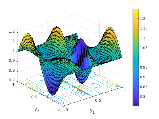
for $t\in\mathbb{R}$ . Note that $A\in\mathcal{M}(\frac{1}{10},\frac{9}{10})$ since $a\in L^{\infty}_{\mathrm{per}}(Y)$ and $\frac{1}{10}\leq a\leq\frac{5}{6}$ a.e. in $\mathbb{R}^{2}$ (note $\lvert\pi^{2}\theta-2\omega\rvert\leq 2$ a.e. in $\mathbb{R}$ ). In particular, in view of Remark 2.1, $A$ satisfies the Cordes condition (2.2) with $\delta=\frac{1}{9}$ . An illustration of the discontinuous function $a$ is provided in Figure 1.

Refer to caption — (a) $a(y_{1},y_{2})$ for $(y_{1},y_{2})\in Y$ .

By Theorem 3.7, noting that $A=C+aM$ with $C:=\mathrm{diag}(1,0)$ and $M:=\mathrm{diag}(-1,1)$ , the invariant measure to $A$ is given by

(5.2)

\displaystyle r(y)=1+M:D^{2}[T(A,a)](y)=1+\frac{1}{8}(\pi^{2}\theta(y_{1})-2\omega(y_{1}))\sin(2\pi y_{2})

for $y=(y_{1},y_{2})\in\mathbb{R}^{2}$ , where we have used that $T(A,a)\in H^{2}_{\mathrm{per},0}(Y)$ (recall Definition 3.2) is given by $[T(A,a)](y)=-\frac{1}{32}\theta(y_{1})\sin(2\pi y_{2})$ for $y=(y_{1},y_{2})\in\mathbb{R}^{2}$ . The effective coefficient matrix $\bar{A}:=\int_{Y}rA$ is then given by

\displaystyle\bar{A}=C+(r,a)_{L^{2}(Y)}M=C+\frac{3}{8}M=\frac{1}{8}\mathrm{diag}(5,3).

A plot of the discontinuous function $r$ is provided in Figure 1.

In our numerical experiment, we use FreeFem++ [21] to approximate $r$ by Theorem 4.1 in combination with the method from Lemma 4.2, where we choose $P_{h}$ to be the finite-dimensional subspace of $H^{1}_{\mathrm{per}}(Y;\mathbb{R}^{2})$ consisting of vector fields whose components are continuous $Y$ -periodic piecewise affine functions with zero mean over $Y$ on a periodic shape-regular triangulation $\mathcal{T}_{h}$ of $\overline{Y}$ into triangles with vertices $\{(ih,jh)\}_{1\leq i,j\leq N}$ where $N=\frac{1}{h}\in\mathbb{N}$ . The integrals in the computation of $c_{h}$ in (4.5) and $\bar{A}_{h}$ in (4.6) have been obtained using the default quadrature formula in FreeFem++ on a fine mesh. The results are presented in Figure 2.

By Lemma 4.2 and Theorem 4.1 we have that $\|r-r_{h}\|_{L^{2}(Y)}\leq C\inf_{w_{h}\in P_{h}}\|D(p-w_{h})\|_{L^{2}(Y)}$ for some constant $C>0$ , where $p\in H^{1}_{\mathrm{per},0}(Y;\mathbb{R}^{2})$ is the function from Lemma 4.2(i). For the approximation of $r$ , we observe convergence of order $\mathcal{O}(h^{s})$ in the $L^{2}(Y)$ -norm for some $s\in(0,1)$ in Figure 2. This indicates that $p\in H^{1+s}(Y)$ in which case we have by standard interpolation inequalities that $\inf_{w_{h}\in P_{h}}\|D(p-w_{h})\|_{L^{2}(Y)}\leq Ch^{s}\|p\|_{H^{1+s}(Y)}$ . In Figure 2, we observe the superconvergence $\|r-r_{h}\|_{L^{2}(Y)}=\mathcal{O}(h)$ for $h=2^{-i}$ , $i\in\mathbb{N}$ , i.e., when there is no element of the triangulation whose interior intersects the line $\{y_{1}=\frac{1}{2}\}$ along which $r$ has a jump.

For the approximation of $\bar{A}$ , we observe that $\lvert\bar{A}-\bar{A}_{h}\rvert=\mathcal{O}(h)$ , and the superconvergence $\lvert\bar{A}-\bar{A}_{h}\rvert=\mathcal{O}(h^{2})$ for $h=2^{-i}$ , $i\in\mathbb{N}$ .

6. Collection of the Proofs

6.1. Proofs for Section 2

Proof of Theorem 2.1.

First, note that there exists a constant $\tilde{c}_{0}=\tilde{c}_{0}(\mathrm{diam}(\Omega),n)>0$ such that $\|v\|_{H^{2}(\Omega)}\leq\tilde{c}_{0}\|\Delta v\|_{L^{2}(\Omega)}$ for any $v\in H^{2}(\Omega)\cap H^{1}_{0}(\Omega)$ . Since $\tilde{f}_{\varepsilon}:=f-L_{\varepsilon}g\in L^{2}(\Omega)$ , we know from Theorem 3 in [27] that there exists a unique function $\tilde{u}_{\varepsilon}\in H^{2}(\Omega)\cap H^{1}_{0}(\Omega)$ such that $L_{\varepsilon}\tilde{u}_{\varepsilon}=\tilde{f}_{\varepsilon}$ a.e. in $\Omega$ , and we have that

\displaystyle\|\tilde{u}_{\varepsilon}\|_{H^{2}(\Omega)}\leq\tilde{c}_{0}C_{\delta}\|\gamma^{\varepsilon}\tilde{f}_{\varepsilon}\|_{L^{2}(\Omega)},

where $C_{\delta}:=(1-\sqrt{1-\delta})^{-1}$ and $\gamma^{\varepsilon}:=\gamma(\frac{\cdot}{\varepsilon})$ with $\gamma$ defined in Remark 2.2. As $\|\gamma\|_{L^{\infty}(\mathbb{R}^{n})}\leq\frac{\Lambda}{\lambda^{2}}$ and $\|L_{\varepsilon}g\|_{L^{2}(\Omega)}\leq c_{1}\|D^{2}g\|_{L^{2}(\Omega)}$ with $c_{1}:=\sqrt{n}\Lambda$ , it follows that $\|\tilde{u}_{\varepsilon}\|_{H^{2}(\Omega)}\leq c_{2}(\|f\|_{L^{2}(\Omega)}+\|g\|_{H^{2}(\Omega)})$ with $c_{2}:=\tilde{c}_{0}(1+c_{1})C_{\delta}\frac{\Lambda}{\lambda^{2}}$ . We find that $u_{\varepsilon}:=\tilde{u}_{\varepsilon}+g\in H^{2}(\Omega)$ is the unique solution to (2.1) in $H^{2}(\Omega)$ and we have the bound $\|u_{\varepsilon}\|_{H^{2}(\Omega)}\leq\|\tilde{u}_{\varepsilon}\|_{H^{2}(\Omega)}+\|g\|_{H^{2}(\Omega)}\leq(c_{2}+1)(\|f\|_{L^{2}(\Omega)}+\|g\|_{H^{2}(\Omega)})$ . ∎

6.2. Proofs for Section 3.1

Proof of Lemma 3.1.

In view of Remark 2.2 and Remark 3.1 we have for any $\varphi\in H^{2}_{\mathrm{per}}(Y)$ that

	$\displaystyle b_{\mu}(\varphi,\varphi)$	$\displaystyle=\\|\mu\varphi-\Delta\varphi\\|_{L^{2}(Y)}^{2}+\left((I_{n}-\gamma A):D^{2}\varphi,\mu\varphi-\Delta\varphi\right)_{L^{2}(Y)}$
		$\displaystyle\geq\\|\mu\varphi-\Delta\varphi\\|_{L^{2}(Y)}^{2}-\sqrt{1-\delta}\\|D^{2}\varphi\\|_{L^{2}(Y)}\\|\mu\varphi-\Delta\varphi\\|_{L^{2}(Y)}.$

Finally, using that for any $\varphi\in H^{2}_{\mathrm{per}}(Y)$ we have that

\displaystyle\|D^{2}\varphi\|_{L^{2}(Y)}^{2}=\|\Delta\varphi\|_{L^{2}(Y)}^{2}\leq\mu^{2}\|\varphi\|_{L^{2}(Y)}^{2}+2\mu\|\nabla\mu\|_{L^{2}(Y)}^{2}+\|\Delta\varphi\|_{L^{2}(Y)}^{2}=\|\mu\varphi-\Delta\varphi\|_{L^{2}(Y)}^{2},

the claimed result follows. ∎

6.3. Proofs for Section 3.2

Proof of Theorem 3.1.

(i) Note that $b_{0}$ is coercive on $H^{2}_{\mathrm{per},0}(Y)$ by Lemma 3.1 and that

(6.1)

\displaystyle\lvert b_{0}(\varphi_{1},\varphi_{2})\rvert=\lvert(\gamma A:D^{2}\varphi_{1},\Delta\varphi_{2})_{L^{2}(Y)}\rvert\leq\sqrt{n}\frac{\Lambda}{\lambda}\|\Delta\varphi_{1}\|_{L^{2}(Y)}\|\Delta\varphi_{2}\|_{L^{2}(Y)}\quad\forall\varphi_{1},\varphi_{2}\in H^{2}_{\mathrm{per},0}(Y),

where we have used Remark 3.1 and that $\gamma\lvert A\rvert=\frac{\mathrm{tr}(A)}{\lvert A\rvert}\leq\frac{n\Lambda}{\sqrt{n}\lambda}=\sqrt{n}\frac{\Lambda}{\lambda}$ almost everywhere. Since $l:H^{2}_{\mathrm{per},0}(Y)\rightarrow\mathbb{R}$ , $l(\varphi):=\int_{Y}\tilde{A}:D^{2}\varphi$ is a bounded linear map with $\lvert l(\varphi)\rvert\leq\sqrt{n}\frac{\Lambda}{\lambda}\|\Delta\varphi\|_{L^{2}(Y)}$ for any $\varphi\in H^{2}_{\mathrm{per},0}(Y)$ , we deduce from the Lax–Milgram theorem that there exists a unique $\psi\in H^{2}_{\mathrm{per},0}(Y)$ such that $b_{0}(\varphi,\psi)=l(\varphi)$ for any $\varphi\in H^{2}_{\mathrm{per},0}(Y)$ and we have the bound

\displaystyle\|\Delta\psi\|_{L^{2}(Y)}^{2}\leq C_{\delta}\,b_{0}(\psi,\psi)=C_{\delta}\,l(\psi)\leq\sqrt{n}\frac{\Lambda}{\lambda}C_{\delta}\|\Delta\psi\|_{L^{2}(Y)}.

(ii) Since $\tilde{r}:=1-\Delta\psi\in L^{2}_{\mathrm{per}}(Y)$ , $\int_{Y}\tilde{r}=1$ , and $(\tilde{r},\tilde{A}:D^{2}\varphi)_{L^{2}(Y)}=l(\varphi)-b_{0}(\varphi,\psi)=0$ for any $\varphi\in H^{2}_{\mathrm{per}}(Y)$ , we have that $\tilde{r}$ is an invariant measure to $\tilde{A}$ . Suppose $\hat{r}\in L^{2}_{\mathrm{per}}(Y)$ is another invariant measure to $\tilde{A}$ . Then, as $\int_{Y}\hat{r}=1$ , there exists a unique $\xi\in H^{2}_{\mathrm{per},0}(Y)$ such that $\Delta\xi=1-\hat{r}$ . Since $b_{0}(\varphi,\xi)=l(\varphi)-(\hat{r},\tilde{A}:D^{2}\varphi)_{L^{2}(Y)}=l(\varphi)$ for any $\varphi\in H^{2}_{\mathrm{per}}(Y)$ , we have that $\xi=\psi$ and thus, $\hat{r}=1-\Delta\psi=\tilde{r}$ . Therefore, $\tilde{r}$ is the unique invariant measure to $\tilde{A}$ .

It remains to show that $\tilde{r}\geq 0$ almost everywhere. For $k\in\mathbb{N}$ we set $a_{k,ij}:=a_{ij}\ast w_{k}$ for $1\leq i,j\leq n$ , where $w_{k}:=k^{n}w(k\,\cdot)$ for some $w\in C_{c}^{\infty}(\mathbb{R}^{n})$ with $w\geq 0$ in $\mathbb{R}^{n}$ and $\int_{\mathbb{R}^{n}}w=1$ . Then, $A_{k}:=(a_{k,ij})_{1\leq i,j\leq n}\in C^{\infty}_{\mathrm{per}}(Y;\mathbb{R}^{n\times n}_{\mathrm{sym}})\cap\mathcal{M}(\lambda,\Lambda)$ for all $k\in\mathbb{N}$ and we have that $\lim_{k\rightarrow\infty}\|A_{k}-A\|_{L^{2}(Y)}=0$ . We set $\gamma_{k}:=\frac{\mathrm{tr}(A_{k})}{\lvert A_{k}\rvert^{2}}\in C^{\infty}_{\mathrm{per}}(Y)$ and note that $\frac{\lambda}{\Lambda^{2}}\leq\gamma_{k}\leq\frac{\Lambda}{\lambda^{2}}$ for any $k\in\mathbb{N}$ , as observed in Remark 2.2. Let $\tilde{r}_{k}\in L^{2}_{\mathrm{per}}(Y)$ be the unique invariant measure to $\tilde{A}_{k}:=\gamma_{k}A_{k}$ . Since $\tilde{A}_{k}\in C^{\infty}_{\mathrm{per}}(Y)$ , we have that $\tilde{r}_{k}\in C^{\infty}_{\mathrm{per}}(Y)$ and it is known (see e.g., [6]) that $\tilde{r}_{k}>0$ in $\mathbb{R}^{n}$ . Setting $q_{k}:=\tilde{r}_{k}\gamma_{k}\in C^{\infty}_{\mathrm{per}}(Y)$ , we have that $q_{k}\geq\frac{\lambda}{\Lambda^{2}}\tilde{r}_{k}>0$ in $\mathbb{R}^{n}$ and, by (i) and the first part of (ii), we find $\|q_{k}\|_{L^{2}(Y)}\leq\frac{\Lambda}{\lambda^{2}}\|\tilde{r}_{k}\|_{L^{2}(Y)}\leq C$ for all $k\in\mathbb{N}$ for some constant $C=C(\lambda,\Lambda,n,\delta)>0$ . Therefore, there exists $q\in L^{2}_{\mathrm{per}}(Y)$ such that, upon passing to a subsequence, $q_{k}\rightharpoonup q$ weakly in $L^{2}(Y)$ . Thus, for any $\varphi\in C^{\infty}_{\mathrm{per}}(Y)$ we have

\displaystyle 0=(q_{k},A_{k}:D^{2}\varphi)_{L^{2}(Y)}=(q_{k},A:D^{2}\varphi)_{L^{2}(Y)}+(q_{k},(A_{k}-A):D^{2}\varphi)_{L^{2}(Y)}\underset{k\rightarrow\infty}{\longrightarrow}(q,A:D^{2}\varphi)_{L^{2}(Y)}.

It follows that $q\in L^{2}_{\mathrm{per}}(Y)$ is a solution to $-D^{2}:(qA)=0$ in $Y$ . Note that $q\geq 0$ a.e. in $\mathbb{R}^{n}$ and $\int_{Y}q\geq\frac{\lambda}{\Lambda^{2}}>0$ as $q_{k}>0$ in $\mathbb{R}^{n}$ and $\int_{Y}q_{k}\geq\frac{\lambda}{\Lambda^{2}}\int_{Y}\tilde{r}_{k}=\frac{\lambda}{\Lambda^{2}}$ for any $k\in\mathbb{N}$ . Recalling that $\gamma>0$ a.e. in $\mathbb{R}^{n}$ , we see that $\int_{Y}\frac{q}{\gamma}=\|\frac{q}{\gamma}\|_{L^{1}(Y)}>0$ . Setting $\tilde{q}:=(\int_{Y}\frac{q}{\gamma})^{-1}\frac{q}{\gamma}\in L^{2}_{\mathrm{per}}(Y)$ and using uniqueness of the invariant measure to $\tilde{A}$ , we see that $\tilde{r}=\tilde{q}\geq 0$ a.e. in $\mathbb{R}^{n}$ .

(iii) This follows immediately from (ii) and the fact that $\frac{\lambda}{\Lambda^{2}}\leq\gamma\leq\frac{\Lambda}{\lambda^{2}}$ a.e. in $\mathbb{R}^{n}$ . Note that the bound (3.3) follows from $\|r\|_{L^{2}(Y)}\leq\frac{\Lambda}{\lambda^{2}}(\gamma,\tilde{r})_{L^{2}(Y)}^{-1}\|\tilde{r}\|_{L^{2}(Y)}$ and $(\gamma,\tilde{r})_{L^{2}(Y)}\geq\frac{\lambda}{\Lambda^{2}}\int_{Y}\tilde{r}=\frac{\lambda}{\Lambda^{2}}$ , where we have used that $\tilde{r}\geq 0$ almost everywhere and $\int_{Y}\tilde{r}=1$ . ∎

Proof of Theorem 3.2.

(i) If $q\in L^{2}_{\mathrm{per}}(Y)$ is a solution to (3.1), then $\int_{Y}f=(f,1)_{L^{2}(Y)}=(q,-A:D^{2}1)_{L^{2}(Y)}=0$ , where $1$ denotes the constant function with value one. Now suppose that $\int_{Y}f=0$ . Then, by Lemma (3.1) and the Lax–Milgram theorem, there exists a unique $\eta\in H^{2}_{\mathrm{per},0}(Y)$ such that $b_{0}(\varphi,\eta)=(f,\varphi)_{L^{2}(Y)}$ for any $\varphi\in H^{2}_{\mathrm{per},0}(Y)$ . Equivalently, since $\int_{Y}f=0$ , we have $b_{0}(\varphi,\eta)=(f,\varphi)_{L^{2}(Y)}$ for any $\varphi\in H^{2}_{\mathrm{per}}(Y)$ . Setting $q:=-\gamma\Delta\eta\in L^{2}_{\mathrm{per}}(Y)$ , we have that $(q,-A:D^{2}\varphi)_{L^{2}(Y)}=b_{0}(\varphi,\eta)=(f,\varphi)_{L^{2}(Y)}$ for any $\varphi\in H^{2}_{\mathrm{per}}(Y)$ , i.e., $q$ is a solution to (3.1).

(ii) Suppose that $q_{1},q_{2}\in L^{2}_{\mathrm{per}}(Y)$ are solutions to (3.1). Then, $w:=q_{1}-q_{2}\in L^{2}_{\mathrm{per}}(Y)$ satisfies $(w,-A:D^{2}\varphi)_{L^{2}(Y)}=0$ for all $\varphi\in H^{2}_{\mathrm{per}}(Y)$ and $\int_{Y}w=c$ . This gives $w=cr$ . Indeed, by uniqueness of $r$ , we see that if $c\neq 0$ then $r=c^{-1}w$ , and if $c=0$ then $r=w+r$ , i.e., $w=0=cr$ .

(iii) Note that $q_{0}=-\gamma\Delta\eta+(\gamma,\Delta\eta)_{L^{2}(Y)}r$ , where $\eta\in H^{2}_{\mathrm{per},0}(Y)$ is as in the proof of (i). By Lemma 3.1 and Remark 3.1 we have $\|\Delta\eta\|_{L^{2}(Y)}^{2}\leq C_{\delta}b_{0}(\eta,\eta)=C_{\delta}(f,\eta)_{L^{2}(Y)}\leq\frac{n}{\pi^{2}}C_{\delta}\|f\|_{L^{2}(Y)}\|\Delta\eta\|_{L^{2}(Y)}$ . Using that $\frac{\lambda}{\Lambda^{2}}\leq\gamma\leq\frac{\Lambda}{\lambda^{2}}$ a.e. in $\mathbb{R}^{n}$ , we see that $\|q_{0}\|_{L^{2}(Y)}\leq\frac{\Lambda}{\lambda^{2}}\left(1+\|r\|_{L^{2}(Y)}\right)\|\Delta\eta\|_{L^{2}(Y)}$ which yields the claimed result in combination with $\|\Delta\eta\|_{L^{2}(Y)}\leq\frac{n}{\pi^{2}}C_{\delta}\|f\|_{L^{2}(Y)}$ . ∎

Proof of Theorem 3.3.

(i,ii) If $v\in H^{2}_{\mathrm{per}}(Y)$ solves (3.2), then $(f,r)_{L^{2}(Y)}=(-A:D^{2}v,r)_{L^{2}(Y)}=0$ . Now suppose $(f,r)_{L^{2}(Y)}=0$ . By the Lax–Milgram theorem, in view of Lemma 3.1, there exists a unique $v\in H^{2}_{\mathrm{per},0}(Y)$ such that $b_{0}(v,\varphi)=(\gamma f,-\Delta\varphi)_{L^{2}(Y)}$ for any $\varphi\in H^{2}_{\mathrm{per},0}(Y)$ . Equivalently, since $-\Delta:H^{2}_{\mathrm{per},0}(Y)\rightarrow L^{2}_{\mathrm{per},0}(Y)$ is a bijection, we have that

(6.2)

\displaystyle(-\gamma A:D^{2}v,\phi)_{L^{2}(Y)}=(\gamma f,\phi)_{L^{2}(Y)}\qquad\forall\phi\in L^{2}_{\mathrm{per},0}(Y).

We claim that this is equivalent to

(6.3)

\displaystyle(-\gamma A:D^{2}v,\phi)_{L^{2}(Y)}=(\gamma f,\phi)_{L^{2}(Y)}\qquad\forall\phi\in L^{2}_{\mathrm{per}}(Y).

Indeed, to see that (6.2) implies (6.3), we write $\phi\in L^{2}_{\mathrm{per}}(Y)$ as $\phi=\phi_{1}+\phi_{2}$ with $\phi_{1}:=\phi-c\tilde{r}\in L^{2}_{\mathrm{per},0}(Y)$ and $\phi_{2}:=c\tilde{r}$ , where $c:=\int_{Y}\phi$ and $\tilde{r}:=(\frac{1}{\gamma},r)_{L^{2}(Y)}^{-1}\frac{r}{\gamma}\in L^{2}_{\mathrm{per}}(Y)$ is the invariant measure to $\tilde{A}:=\gamma A$ , and use that $(-\tilde{A}:D^{2}v,\phi_{2})_{L^{2}(Y)}=0=c(\frac{1}{\gamma},r)_{L^{2}(Y)}^{-1}(f,r)_{L^{2}(Y)}=(\gamma f,\phi_{2})_{L^{2}(Y)}$ . Noting that (6.3) is equivalent to $-\gamma A:D^{2}v=\gamma f$ a.e. in $\mathbb{R}^{n}$ , which in turn is equivalent to $-A:D^{2}v=f$ a.e. in $\mathbb{R}^{n}$ since $\gamma\geq\frac{\lambda}{\Lambda^{2}}>0$ a.e. in $\mathbb{R}^{n}$ , we immediately obtain (i)–(ii).

(iii) Note that $v_{0}$ is the unique element in $H^{2}_{\mathrm{per},0}(Y)$ such that $b_{0}(v_{0},\varphi)=-(\gamma f,\Delta\varphi)_{L^{2}(Y)}$ for any $\varphi\in H^{2}_{\mathrm{per}}(Y)$ . Hence, $\|\Delta v_{0}\|_{L^{2}(Y)}^{2}\leq C_{\delta}b_{0}(v_{0},v_{0})=-C_{\delta}(\gamma f,\Delta v_{0})_{L^{2}(Y)}\leq\frac{\Lambda}{\lambda^{2}}C_{\delta}\|f\|_{L^{2}(Y)}\|\Delta v_{0}\|_{L^{2}(Y)}$ by Lemma 3.1 and Remark 2.2. ∎

6.4. Proofs for Section 3.3

Proof of Theorem 3.4.

First, recall that by the uniform $H^{2}$ -bound (2.3) there exists a function $u\in H^{2}(\Omega)$ with $u-g\in H^{1}_{0}(\Omega)$ such that, upon passing to a subsequence, (3.5) holds. Passing to the limit in (3.10) and using (3.11) we find that $u$ is a solution to (3.12). Noting that

\displaystyle\lambda\lvert\xi\rvert^{2}=\lambda\lvert\xi\rvert^{2}(r,1)_{L^{2}(Y)}\leq(r,A\xi\cdot\xi)_{L^{2}(Y)}=\bar{A}\xi\cdot\xi\leq\Lambda\lvert\xi\rvert^{2}(r,1)_{L^{2}(Y)}=\Lambda\lvert\xi\rvert^{2}\quad\forall\xi\in\mathbb{R}^{n},

where we have used that $r\geq 0$ almost everywhere and $A\in\mathcal{M}(\lambda,\Lambda)$ , we see that $u$ is the unique solution in $H^{2}(\Omega)$ to (3.12). We conclude that the whole sequence $(u_{\varepsilon})_{\varepsilon>0}$ convergences weakly in $H^{2}(\Omega)$ to $u$ . ∎

6.5. Proofs for Section 3.4

Proof of Theorem 3.5.

We have $r_{\varepsilon}:=u_{\varepsilon}-u-\varepsilon^{2}(\eta_{\varepsilon}+\theta_{\varepsilon})\in H^{2}(\Omega)\cap H^{1}_{0}(\Omega)$ and $L_{\varepsilon}r_{\varepsilon}=\varepsilon A^{\varepsilon}:P_{\varepsilon}$ . By the proof of Theorem 2.1 and using that $\gamma\lvert A\rvert=\frac{\mathrm{tr}(A)}{\lvert A\rvert}\leq\frac{n\Lambda}{\sqrt{n}\lambda}=\sqrt{n}\frac{\Lambda}{\lambda}$ almost everywhere, we then have the bound

\displaystyle\|r_{\varepsilon}\|_{H^{2}(\Omega)}\leq C_{\delta}\tilde{c}_{0}\|\gamma^{\varepsilon}L_{\varepsilon}r_{\varepsilon}\|_{L^{2}(\Omega)}\leq\varepsilon C_{\delta}\tilde{c}_{0}\|\gamma\lvert A\rvert\|_{L^{\infty}(\mathbb{R}^{n})}\|P_{\varepsilon}\|_{L^{2}(\Omega)}\leq\varepsilon C_{\delta}\tilde{c}_{0}\sqrt{n}\frac{\Lambda}{\lambda}\|P_{\varepsilon}\|_{L^{2}(\Omega)},

where $C_{\delta}:=(1-\sqrt{1-\delta})^{-1}$ and $\tilde{c}_{0}=\tilde{c}_{0}(\mathrm{diam}(\Omega),n)>0$ is as in the proof of Theorem 2.1. The claim follows with $c_{0}:=\tilde{c}_{0}\sqrt{n}$ . ∎

Proof of Theorem 3.6.

We set $d_{\varepsilon}:=r_{\varepsilon}+2\varepsilon(z_{\varepsilon}-\varepsilon^{2}(\tilde{\eta}_{\varepsilon}+\tilde{\theta}_{\varepsilon}))$ where $r_{\varepsilon}:=u_{\varepsilon}-u-\varepsilon^{2}(\eta_{\varepsilon}+\theta_{\varepsilon})$ . We have that $d_{\varepsilon}\in H^{2}(\Omega)\cap H^{1}_{0}(\Omega)$ and, writing $c_{j}^{kl}:=(Ae_{j}\cdot\nabla v_{kl},r)_{L^{2}(Y)}$ for $1\leq j,k,l\leq n$ , there holds

	$\displaystyle L_{\varepsilon}d_{\varepsilon}$	$\displaystyle=\varepsilon A^{\varepsilon}:P_{\varepsilon}+2\varepsilon\left(-\sum_{j,k,l=1}^{n}c_{j}^{kl}\partial^{3}_{jkl}u+\varepsilon^{2}A^{\varepsilon}:D^{2}\tilde{\eta}_{\varepsilon}\right)$
		$\displaystyle=\varepsilon A^{\varepsilon}:P_{\varepsilon}-2\varepsilon\sum_{j,k,l=1}^{n}[c_{j}^{kl}-A:D^{2}\chi_{jkl}]^{\varepsilon}\partial^{3}_{jkl}u+2\varepsilon^{2}\sum_{i,j=1}^{n}a_{ij}^{\varepsilon}(2[\partial_{i}X]^{\varepsilon}:D^{3}(\partial_{j}u)+\varepsilon X^{\varepsilon}:D^{3}(\partial^{2}_{ij}u))$
		$\displaystyle=\varepsilon^{2}A^{\varepsilon}:Q_{\varepsilon},$

where we have used that $\chi_{jkl}=T(A,Ae_{j}\cdot\nabla v_{kl})$ and $L_{\varepsilon}r_{\varepsilon}=\varepsilon A^{\varepsilon}:P_{\varepsilon}$ with $P_{\varepsilon}$ defined as in Theorem 3.5. By the proof of Theorem 2.1 and using that $\gamma\lvert A\rvert=\frac{\mathrm{tr}(A)}{\lvert A\rvert}\leq\frac{n\Lambda}{\sqrt{n}\lambda}=\sqrt{n}\frac{\Lambda}{\lambda}$ almost everywhere, we then have the bound

\displaystyle\|d_{\varepsilon}\|_{H^{2}(\Omega)}\leq C_{\delta}\tilde{c}_{0}\|\gamma^{\varepsilon}L_{\varepsilon}d_{\varepsilon}\|_{L^{2}(\Omega)}\leq\varepsilon^{2}C_{\delta}\tilde{c}_{0}\|\gamma\lvert A\rvert\|_{L^{\infty}(\mathbb{R}^{n})}\|Q_{\varepsilon}\|_{L^{2}(\Omega)}\leq\varepsilon^{2}C_{\delta}\tilde{c}_{0}\sqrt{n}\frac{\Lambda}{\lambda}\|Q_{\varepsilon}\|_{L^{2}(\Omega)},

6.6. Proofs for Section 3.5

The proofs of Theorem 3.7 and Theorem 3.8 are almost identical to the proofs in [17] and hence omitted.

6.7. Proofs for Section 4

Proof of Lemma 4.1.

In view of Lemma 3.1, we note that existence and uniqueness of $\psi_{h}\in\Psi_{h}$ satisfying (4.3) follows from the Lax–Milgram theorem. Noting that $\psi-\psi_{h}\in H^{2}_{\mathrm{per},0}(Y)$ and using Lemma 3.1, Galerkin orthogonality, and (6.1), we have for any $\varphi_{h}\in\Psi_{h}$ that

	$\displaystyle C_{\delta}^{-1}\\|\Delta(\psi-\psi_{h})\\|_{L^{2}(Y)}^{2}$	$\displaystyle\leq b_{0}(\psi-\psi_{h},\psi-\psi_{h})$
		$\displaystyle=b_{0}(\psi-\varphi_{h},\psi-\psi_{h})\leq\sqrt{n}\frac{\Lambda}{\lambda}\\|\Delta(\psi-\varphi_{h})\\|_{L^{2}(Y)}\\|\Delta(\psi-\psi_{h})\\|_{L^{2}(Y)},$

which yields the claimed result. Note that $\tilde{r}-\tilde{r}_{h}=-\Delta(\psi-\psi_{h})$ since $\tilde{r}_{h}=1-\Delta\psi_{h}$ and $\tilde{r}=1-\Delta\psi$ by Theorem 3.1. ∎

Proof of Lemma 4.2.

First, we note that for any $w\in H^{1}_{\mathrm{per}}(Y;\mathbb{R}^{n})$ there holds

\displaystyle\|\nabla\cdot w\|_{L^{2}(Y)}^{2}+\frac{1}{2}\|Dw-Dw^{\mathrm{T}}\|_{L^{2}(Y)}^{2}=\|Dw\|_{L^{2}(Y)}^{2}+\|\nabla\cdot w\|_{L^{2}(Y)}^{2}-(Dw,Dw^{\mathrm{T}})_{L^{2}(Y)}=\|Dw\|_{L^{2}(Y)}^{2},

where the second equality follows from integration by parts and a density argument. We find that

(6.4)

\displaystyle\begin{split}b(w,w)&=\|Dw\|_{L^{2}(Y)}^{2}+((\tilde{A}-I_{n}):Dw,\nabla\cdot w)_{L^{2}(Y)}\\ &\geq\|Dw\|_{L^{2}(Y)}^{2}-\sqrt{1-\delta}\|\nabla\cdot w\|_{L^{2}(Y)}\|Dw\|_{L^{2}(Y)}\geq C_{\delta}^{-1}\|Dw\|_{L^{2}(Y)}^{2}\end{split}

for any $w\in H^{1}_{\mathrm{per}}(Y;\mathbb{R}^{n})$ , where $C_{\delta}=(1-\sqrt{1-\delta})^{-1}$ . Further, using that $\|\gamma\lvert A\rvert\|_{L^{\infty}(\mathbb{R}^{n})}\leq\sqrt{n}\frac{\Lambda}{\lambda}$ and setting $C_{n,\lambda,\Lambda}:=1+\sqrt{n}\frac{\Lambda}{\lambda}$ , we have for any $w\in H^{1}_{\mathrm{per}}(Y;\mathbb{R}^{n})$ that

(6.5)

\displaystyle\begin{split}\lvert b(w,\tilde{w})\rvert&\leq\sqrt{n}\frac{\Lambda}{\lambda}\|Dw\|_{L^{2}(Y)}\|\nabla\cdot\tilde{w}\|_{L^{2}(Y)}+\frac{1}{2}\|Dw-Dw^{\mathrm{T}}\|_{L^{2}(Y)}\|D\tilde{w}-D\tilde{w}^{\mathrm{T}}\|_{L^{2}(Y)}\\ &\leq C_{n,\lambda,\Lambda}\|Dw\|_{L^{2}(Y)}\|D\tilde{w}\|_{L^{2}(Y)},\end{split}

where we have used in the second inequality that $\frac{1}{2}\|Dw-Dw^{\mathrm{T}}\|_{L^{2}(Y)}^{2}\leq\|Dw\|_{L^{2}(Y)}^{2}$ for any $w\in H^{1}_{\mathrm{per}}(Y;\mathbb{R}^{n})$ . Since $w\mapsto\|Dw\|_{L^{2}(Y)}$ defines a norm on $H^{1}_{\mathrm{per},0}(Y;\mathbb{R}^{n})$ , it follows that $b$ defines a bounded coercive bilinear form on $H^{1}_{\mathrm{per},0}(Y;\mathbb{R}^{n})$ . By the Lax–Milgram theorem, using that $w\mapsto(\gamma,A:Dw)_{L^{2}(Y)}$ defines a bounded linear functional on $H^{1}_{\mathrm{per},0}(Y;\mathbb{R}^{n})$ , we have that there exist unique $p\in H^{1}_{\mathrm{per},0}(Y;\mathbb{R}^{n})$ and $p_{h}\in P_{h}$ such that

\displaystyle b(w,p)=(\gamma,A:Dw)_{L^{2}(Y)}\quad\forall w\in H^{1}_{\mathrm{per},0}(Y;\mathbb{R}^{n}),\qquad b(w_{h},p_{h})=(\gamma,A:Dw_{h})_{L^{2}(Y)}\quad\forall w_{h}\in P_{h}.

Noting that for any $\varphi\in H^{2}_{\mathrm{per}}(Y)$ we have that $\nabla\varphi\in H^{1}_{\mathrm{per},0}(Y;\mathbb{R}^{n})$ , we see that

\displaystyle(1-\nabla\cdot p,-\tilde{A}:D^{2}\varphi)_{L^{2}(Y)}=b(\nabla\varphi,p)-(\gamma,A:D^{2}\varphi)_{L^{2}(Y)}=0\qquad\forall\varphi\in H^{2}_{\mathrm{per}}(Y).

Therefore, using that $\nabla\cdot p\in L^{2}_{\mathrm{per},0}(Y)$ , we have that $\tilde{r}=1-\nabla\cdot p$ . It only remains to prove (iii). Noting that $p-p_{h}\in H^{1}_{\mathrm{per},0}(Y;\mathbb{R}^{n})$ and using (6.4), Galerkin orthogonality, and (6.5), we have that

	$\displaystyle C_{\delta}^{-1}\\|D(p-p_{h})\\|_{L^{2}(Y)}^{2}$	$\displaystyle\leq b(p-p_{h},p-p_{h})$
		$\displaystyle=b(p-w_{h},p-p_{h})\leq C_{n,\lambda,\Lambda}\\|D(p-w_{h})\\|_{L^{2}(Y)}\\|D(p-p_{h})\\|_{L^{2}(Y)}$

for any $w_{h}\in P_{h}$ . Since $\|\nabla\cdot(p-p_{h})\|_{L^{2}(Y)}\leq\|D(p-p_{h})\|_{L^{2}(Y)}$ , this yields the claimed result. Note that $\tilde{r}-\tilde{r}_{h}=-\nabla\cdot(p-p_{h})$ since $\tilde{r}_{h}=1-\nabla\cdot p_{h}$ and $\tilde{r}=1-\nabla\cdot p$ . ∎

Proof of Theorem 4.1.

First, recall that $r=c^{-1}\gamma\tilde{r}$ with $c:=(\gamma,\tilde{r})_{L^{2}(Y)}\in[\frac{\lambda}{\Lambda^{2}},\frac{\Lambda}{\lambda^{2}}]$ , where we have used the bounds on $\gamma$ from Remark 2.2, $\int_{Y}\tilde{r}=1$ , and $\tilde{r}\geq 0$ almost everywhere. Noting that $\lvert c-c_{h}\rvert\leq\frac{\Lambda}{\lambda^{2}}\|\tilde{r}-\tilde{r}_{h}\|_{L^{2}(Y)}$ , we see that $c_{h}\rightarrow c$ and hence, $r_{h}$ is well-defined for $h>0$ sufficiently small. Further, for $h>0$ sufficiently small, there holds

\displaystyle\|r-r_{h}\|_{L^{2}(Y)}=\|c^{-1}\gamma\tilde{r}-c_{h}^{-1}\gamma\tilde{r}_{h}\|_{L^{2}(Y)}\leq c_{h}^{-1}\|\gamma(\tilde{r}-\tilde{r}_{h})\|_{L^{2}(Y)}+\lvert c^{-1}-c_{h}^{-1}\rvert\,\|\gamma\tilde{r}\|_{L^{2}(Y)},

and using that $\gamma\tilde{r}=cr$ , we find

	$\displaystyle\\|r-r_{h}\\|_{L^{2}(Y)}$	$\displaystyle\leq c_{h}^{-1}\left(\\|\gamma(\tilde{r}-\tilde{r}_{h})\\|_{L^{2}(Y)}+\lvert c-c_{h}\rvert\,\\|r\\|_{L^{2}(Y)}\right)$
		$\displaystyle\leq\frac{\Lambda}{\lambda^{2}}c_{h}^{-1}\left(\\|\tilde{r}-\tilde{r}_{h}\\|_{L^{2}(Y)}+\frac{\Lambda}{\lambda^{2}}\\|\tilde{r}-\tilde{r}_{h}\\|_{L^{2}(Y)}\\|r\\|_{L^{2}(Y)}\right)$

Noting that $c_{h}^{-1}\leq\frac{\Lambda^{2}}{\lambda}+1$ for $h>0$ sufficiently small completes the proof. ∎

Proof of Lemma 4.3.

We have $\lvert\bar{A}-\bar{A}_{h}\rvert=\left\lvert\int_{Y}(r-r_{h})A\right\rvert\leq\int_{Y}\lvert r-r_{h}\rvert\lvert A\rvert\leq\sqrt{n}\Lambda\|r-r_{h}\|_{L^{1}(Y)}$ , and the claim follows. ∎

Proof of Lemma 4.4.

The proof of this result is analogous to the proof of Lemma 3.4 in [9] and hence omitted. ∎

Acknowledgments

The author gratefully acknowledges helpful conversations with Professor Yves Capdeboscq (Université de Paris) and Professor Hung V. Tran (University of Wisconsin Madison) during the preparation of this work.

References

[1] S. Armstrong, B. Fehrman, and J. Lin. Green function and invariant measure estimates for nondivergence form elliptic homogenization, 2022. arXiv:2211.13279 [math.AP].
[2] S. Armstrong and J. Lin. Optimal quantitative estimates in stochastic homogenization for elliptic equations in nondivergence form. Arch. Ration. Mech. Anal., 225(2):937–991, 2017.
[3] S. N. Armstrong and C. K. Smart. Quantitative stochastic homogenization of elliptic equations in nondivergence form. Arch. Ration. Mech. Anal., 214(3):867–911, 2014.
[4] M. Avellaneda and F.-H. Lin. Compactness methods in the theory of homogenization. II. Equations in nondivergence form. Comm. Pure Appl. Math., 42(2):139–172, 1989.
[5] M. Bebendorf. A note on the Poincaré inequality for convex domains. Z. Anal. Anwendungen, 22(4):751–756, 2003.
[6] A. Bensoussan, J.-L. Lions, and G. Papanicolaou. Asymptotic analysis for periodic structures. AMS Chelsea Publishing, Providence, RI, 2011. Corrected reprint of the 1978 original.
[7] V. I. Bogachev and S. V. Shaposhnikov. Integrability and continuity of solutions to double divergence form equations. Ann. Mat. Pura Appl. (4), 196(5):1609–1635, 2017.
[8] F. Camilli and C. Marchi. Rates of convergence in periodic homogenization of fully nonlinear uniformly elliptic PDEs. Nonlinearity, 22(6):1481–1498, 2009.
[9] Y. Capdeboscq, T. Sprekeler, and E. Süli. Finite element approximation of elliptic homogenization problems in nondivergence-form. ESAIM Math. Model. Numer. Anal., 54(4):1221–1257, 2020.
[10] H. O. Cordes. Über die erste Randwertaufgabe bei quasilinearen Differentialgleichungen zweiter Ordnung in mehr als zwei Variablen. Math. Ann., 131:278–312, 1956.
[11] B. Engquist and P. E. Souganidis. Asymptotic and numerical homogenization. Acta Numer., 17:147–190, 2008.
[12] C. Finlay and A. M. Oberman. Approximate homogenization of convex nonlinear elliptic PDEs. Commun. Math. Sci., 16(7):1895–1906, 2018.
[13] P. Freese, D. Gallistl, D. Peterseim, and T. Sprekeler. Computational multiscale methods for nondivergence-form elliptic partial differential equations, 2023. arXiv:2211.13731 [math.NA].
[14] B. D. Froese and A. M. Oberman. Numerical averaging of non-divergence structure elliptic operators. Commun. Math. Sci., 7(4):785–804, 2009.
[15] D. Gallistl. Variational formulation and numerical analysis of linear elliptic equations in nondivergence form with Cordes coefficients. SIAM J. Numer. Anal., 55(2):737–757, 2017.
[16] D. Gallistl, T. Sprekeler, and E. Süli. Mixed Finite Element Approximation of Periodic Hamilton–Jacobi–Bellman Problems With Application to Numerical Homogenization. Multiscale Model. Simul., 19(2):1041–1065, 2021.
[17] X. Guo, T. Sprekeler, and H. V. Tran. Characterizations of diffusion matrices in homogenization of elliptic equations in nondivergence-form, 2022. arXiv:2201.01974 [math.AP].
[18] X. Guo and H. V. Tran. Stochastic integrability of heat-kernel bounds for random walks in a balanced random environment, 2022. arXiv:2209.14293 [math.PR].
[19] X. Guo and H. V. Tran. Optimal convergence rates in stochastic homogenization in a balanced random environment, 2023. arXiv:2301.01267 [math.PR].
[20] X. Guo, H. V. Tran, and Y. Yu. Remarks on optimal rates of convergence in periodic homogenization of linear elliptic equations in non-divergence form. SN Partial Differ. Equ. Appl., 1(15), 2020.
[21] F. Hecht. New development in freefem++. J. Numer. Math., 20(3-4):251–265, 2012.
[22] V. V. Jikov, S. M. Kozlov, and O. A. Oleĭnik. Homogenization of differential operators and integral functionals. Springer-Verlag, Berlin, 1994. Translated from the Russian.
[23] W. Jing and Y. Zhang. On the periodic homogenization of elliptic equations in non-divergence form with large drifts, 2023. arXiv:2302.01157 [math.AP].
[24] E. L. Kawecki and T. Sprekeler. Discontinuous Galerkin and C0-IP finite element approximation of periodic Hamilton-Jacobi-Bellman-Isaacs problems with application to numerical homogenization. ESAIM Math. Model. Numer. Anal., 56(2):679–704, 2022.
[25] S. Kim and K.-A. Lee. Higher order convergence rates in theory of homogenization: equations of non-divergence form. Arch. Ration. Mech. Anal., 219(3):1273–1304, 2016.
[26] M. V. Safonov. Non-divergence elliptic equations of second order with unbounded drift. In Nonlinear partial differential equations and related topics, volume 229 of Amer. Math. Soc. Transl. Ser. 2, pages 211–232. Amer. Math. Soc., Providence, RI, 2010.
[27] I. Smears and E. Süli. Discontinuous Galerkin finite element approximation of nondivergence form elliptic equations with Cordès coefficients. SIAM J. Numer. Anal., 51(4):2088–2106, 2013.
[28] T. Sprekeler and H. V. Tran. Optimal convergence rates for elliptic homogenization problems in nondivergence-form: analysis and numerical illustrations. Multiscale Model. Simul., 19(3):1453–1473, 2021.
[29] G. Talenti. Sopra una classe di equazioni ellittiche a coefficienti misurabili. Ann. Mat. Pura Appl. (4), 69:285–304, 1965.

Homogenization of nondivergence-form elliptic equations with discontinuous coefficients and finite element approximation of the homogenized problem

Abstract.

Key words and phrases:

2010 Mathematics Subject Classification

1. Introduction

2. Framework

Remark 2.1.

Remark 2.2.

Theorem 2.1 (well-posedness and uniform H2H^{2}-bound).

3. Homogenization

3.1. Preliminaries

Lemma 3.1 (the bilinear form bμb_{\mu}).

Remark 3.1.

3.2. Periodic problems and invariant measures

Definition 3.1 (invariant measure).

Theorem 3.1 (existence, uniqueness and properties of invariant measures).

Theorem 3.2 (analysis of the problem (3.1)).

Theorem 3.3 (analysis of the problem (3.2)).

3.3. The convergence result

Remark 3.2.

Theorem 3.4 (convergence result).

3.4. Corrector estimates

Definition 3.2 (the notation T⁡(A,a)T(A,a)).

Theorem 3.5 (an 𝒪⁡(ε)\mathcal{O}(\varepsilon) corrector estimate in the H2H^{2}-norm).

Remark 3.3.

Remark 3.4.

Corollary 3.1 (L∞L^{\infty}-rate in dimension n≤3n\leq 3).

Theorem 3.6 (an 𝒪⁡(ε2)\mathcal{O}(\varepsilon^{2}) corrector estimate in the H2H^{2}-norm).

Remark 3.5.

Corollary 3.2 (L∞L^{\infty}-bound in dimension n≤3n\leq 3).

3.5. Type-ε2\varepsilon^{2} diffusion matrices

Definition 3.3 (type-ε2\varepsilon^{2} and type-ε\varepsilon diffusion matrices).

Theorem 3.7 (diffusion matrices A=C+a​MA=C+aM are type-ε2\varepsilon^{2}).

Theorem 3.8 (characterization of type-ε2\varepsilon^{2} diagonal diffusion matrices for n=2n=2).

Remark 3.6.

4. Numerical Methods

4.1. Finite element approximation of the invariant measure

4.1.1. Approximation of r~\tilde{r} via Hper,02​(Y)H^{2}_{\mathrm{per},0}(Y)-conforming FEM for ψ\psi

Lemma 4.1 (approximation of r~\tilde{r} via Hper,02​(Y)H^{2}_{\mathrm{per},0}(Y)-conforming FEM for ψ\psi).

4.1.2. Approximation of r~\tilde{r} via Hper,01​(Y,ℝn)H^{1}_{\mathrm{per},0}(Y;\mathbb{R}^{n})-conforming FEM

Lemma 4.2 (approximation of r~\tilde{r} via Hper,01​(Y,ℝn)H^{1}_{\mathrm{per},0}(Y;\mathbb{R}^{n})-conforming FEM).

4.1.3. Approximation of rr

Theorem 4.1 (approximation of rr).

4.2. Approximation of the homogenized problem

Lemma 4.3 (approximation of A¯\bar{A}).

Lemma 4.4 (approximation of uu).

5. Numerical Experiments

6. Collection of the Proofs

6.1. Proofs for Section 2

Proof of Theorem 2.1.

6.2. Proofs for Section 3.1

Proof of Lemma 3.1.

6.3. Proofs for Section 3.2

Proof of Theorem 3.1.

Proof of Theorem 3.2.

Proof of Theorem 3.3.

6.4. Proofs for Section 3.3

Proof of Theorem 3.4.

6.5. Proofs for Section 3.4

Proof of Theorem 3.5.

Proof of Theorem 3.6.

6.6. Proofs for Section 3.5

6.7. Proofs for Section 4

Proof of Lemma 4.1.

Proof of Lemma 4.2.

Proof of Theorem 4.1.

Proof of Lemma 4.3.

Proof of Lemma 4.4.

Acknowledgments

References

Theorem 2.1 (well-posedness and uniform $H^{2}$ -bound).

Lemma 3.1 (the bilinear form $b_{\mu}$ ).

Definition 3.2 (the notation $T(A,a)$ ).

Theorem 3.5 (an $\mathcal{O}(\varepsilon)$ corrector estimate in the $H^{2}$ -norm).

Corollary 3.1 ( $L^{\infty}$ -rate in dimension $n\leq 3$ ).

Theorem 3.6 (an $\mathcal{O}(\varepsilon^{2})$ corrector estimate in the $H^{2}$ -norm).

Corollary 3.2 ( $L^{\infty}$ -bound in dimension $n\leq 3$ ).

3.5. Type- $\varepsilon^{2}$ diffusion matrices

Definition 3.3 (type- $\varepsilon^{2}$ and type- $\varepsilon$ diffusion matrices).

Theorem 3.7 (diffusion matrices $A=C+aM$ are type- $\varepsilon^{2}$ ).

Theorem 3.8 (characterization of type- $\varepsilon^{2}$ diagonal diffusion matrices for $n=2$ ).

4.1.1. Approximation of $\tilde{r}$ via $H^{2}_{\mathrm{per},0}(Y)$ -conforming FEM for $\psi$

Lemma 4.1 (approximation of $\tilde{r}$ via $H^{2}_{\mathrm{per},0}(Y)$ -conforming FEM for $\psi$ ).

4.1.2. Approximation of $\tilde{r}$ via $H^{1}_{\mathrm{per},0}(Y;\mathbb{R}^{n})$ -conforming FEM

Lemma 4.2 (approximation of $\tilde{r}$ via $H^{1}_{\mathrm{per},0}(Y;\mathbb{R}^{n})$ -conforming FEM).

4.1.3. Approximation of $r$

Theorem 4.1 (approximation of $r$ ).

Lemma 4.3 (approximation of $\bar{A}$ ).

Lemma 4.4 (approximation of $u$ ).