Higher-order Process Matrix Tomography of a passively-stable Quantum SWITCHPreprint: APS/123-QED

The expression quantum process is a general term used to refer to the dynamics of quantum systems, and its precise meaning may depend on the context. For instance, when analysing transformations between quantum states, quantum process refers to a quantum channel, which may be unitary (associated with closed quantum systems and mathematically described by unitary operators) or non-unitary (associated with open quantum systems and mathematically described by Completely Positive Trace Preserving (CPTP) linear maps). In this scenario of transformations between states, one can experimentally determine the dynamics by means of what is known as quantum process tomography Chuang and Nielsen 1997; Poyatos et al. 1997; O’Brien et al. 2004. To do so, a complete set of known quantum states is fed into an unknown quantum process $\mathcal{E}$ and a complete set of measurements is performed on the output of the underlying process for each input state Rozema et al. 2014. When performing standard process tomography, one reconstructs, for example, the chi matrix $\chi$, which takes quantum sates as inputs and returns quantum states as outputs Nielsen and Chuang 2005. The chi matrix is often called a process matrix; however, we stress that this chi or process matrix is different from the process matrices discussed in the field of HOQO and ICO, the case which we address here.

In this work, we analyse transformations between quantum channels, hence we use the word process to describe the dynamics between quantum operations. An operation that transforms a quantum operation is sometimes referred to as a higher-order quantum operation. Such operations have found applications in several branches of quantum information processing Gutoski and Watrous 2007; Chiribella et al. 2008; Chiribella et al. 2009; Bisio et al. 2010; Sedlák et al. 2019; Quintino et al. 2019; Bavaresco et al. 2022. The formalism of higher-order transformations, is also particularly useful for describing quantum processes which may not respect a definite causal order, such as the notorious quantum SWITCH Chiribella et al. 2013; Chiribella 2012, the main object analysed in this work. In its most general form, the quantum SWITCH is a process that, transforms a pair of unitary operators $(U_{A},U_{B})$ into another operator which is a coherent superposition of the composition $U_{A}U_{B}$ and $U_{B}U_{A}$. In mathematical terms, the quantum SWITCH is the transformation

where the first system of the RHS of Eq. 1 is referred to as the control system, since the order in which $U_{A}$ and $U_{B}$ will be performed may be controlled by setting the control qubit state. The second system is referred to the target system, since it is the system on which the unitary operators act.

Higher-order transformations such as the quantum SWITCH may be conveniently described by means of a process matrix Oreshkov et al. 2012, a formalism which is heavily based on the Choi-Jamiołkowski (CJ) isomorphism Jamiołkowski 1972; Choi 1975, a method to represent linear maps as linear operators, and linear operators as vectors. Let $\mathcal{H}_{\text{in}}$ and $\mathcal{H}_{\text{out}}$ be finite linear (Hilbert) spaces associated with the input and output. Let $U:\mathcal{H}_{\text{in}}\to\mathcal{H}_{\text{out}}$ be a linear operator, its process vector $|U\rangle\hskip-2.27621pt\rangle\in\mathcal{H}_{\text{in}}\otimes\mathcal{H}_{\text{out}}$ is the defined as²² 2 Upper-indices on vectors and operators will be used to indicate where these objects act. For instance, in $|U\rangle\hskip-2.27621pt\rangle^{\mathcal{H}_{\text{in}}\mathcal{H}_{\text{out}}}$, the upper indices indicate that $|U\rangle\hskip-2.27621pt\rangle\in\mathcal{H}_{\text{in}}\otimes\mathcal{H}_{\text{out}}$. Whenever clear from context, we might drop the upper indices to avoid an overly heavy notation.

where $\{\ket{i}\}_{i}$ is the computational basis. Notice that, the Choi vector of the identity operator is given by

which is equivalent to a maximally entangled state up to normalisation.

Let $\mathcal{L}(\mathcal{H})$ be the set of all linear operators acting on $\mathcal{H}$. Let $\mathcal{C}:\mathcal{L}(\mathcal{H}_{\text{in}})\to\mathcal{L}(\mathcal{H}_{\text{out}})$ be a linear map, its Choi operator $C\in\mathcal{L}(\mathcal{H}_{\text{in}}\otimes\mathcal{H}_{\text{out}})$ is defined as

Then, the action of any linear map $\mathcal{C}$ on a state $\rho$ can be written in terms of the Choi operator $C$ as

where $\rho^{T}$ is the transpose of $\rho$ in the computational basis and $\rho$ is an arbitrary density operator acting on $\mathcal{H}_{\text{in}}$.

The Choi-Jamiołkowski isomorphism is very useful to represent quantum operations, due to the fact that a linear map $\mathcal{C}:\mathcal{L}(\mathcal{H}_{\text{in}})\to\mathcal{L}(\mathcal{H}_{\text{out}})$ is completely positive if and only if its Choi operator $C\in\mathcal{L}(\mathcal{H}_{\text{in}}\otimes\mathcal{H}_{\text{out}})$ respects $C\geq 0$, and the map $\mathcal{C}$ is trace-preserving if and only if $\Tr_{\text{out}}(C)=\mathds{1}^{\mathcal{H}_{\text{in}}}$. Since quantum channels are completely positive trace-preserving maps, all quantum channels have a simple and direct characterisation in terms of their Choi operators. Before finishing this subsection we also remark that if $\mathcal{C}$ is a unitary channel, that is $\mathcal{C}(\rho)=U\rho U^{\dagger}$ for some unitary operator $U$, direct calculation shows that its Choi operator may be written as $C=|U\rangle\hskip-2.27621pt\rangle\hskip-1.13809pt\langle\hskip-2.27621pt\langle U|$, where $|U\rangle\hskip-2.27621pt\rangle$ is defined in Eq. 2.

A quantum instrument is a quantum operation which has a classical and a quantum output, and it formalises the concept of a quantum measurement which has a post-measurement quantum state. Mathematically, a set of linear maps $\{\mathcal{C}_{i}\}_{i}$, $\mathcal{C}_{i}:\mathcal{L}(\mathcal{H}_{\text{in}})\to\mathcal{L}(\mathcal{H}_{\text{out}})$ is a quantum instrument if all $\mathcal{C}_{i}$ are completely positive and $\mathcal{C}:=\penalty\ \sum_{i}\mathcal{C}_{i}$ is trace preserving. In the Choi operator picture, this is equivalent to having $C_{i}\geq 0$ and $\Tr_{\text{out}}\left(\sum_{i}C_{i}\right)=\mathds{1}^{\mathcal{H}_{\text{in}}}$. A simple and useful class of quantum instrument is the class of measure-and-reprepare instruments. In its most basic form, a measure and reprepare instrument simply performs a measurement described by the operators³³ 3 A set of operators $\{M_{i}\}$ represents a quantum measurement (that is, it is a POVM) if $M_{i}\geq 0$ and $\sum_{i}M_{i}=\mathds{1}$. $\{M_{i}\}$, and reprepares some fixed state $\sigma$. Its linear map is described by $\mathcal{R}_{i}(\rho):=\Tr(\rho\, M_i)\sigma$, and its Choi operators are given by $R_{i}\in\mathcal{L}\left(\mathcal{H}_{\text{in}}\otimes\mathcal{H}_{\text{out}}\right)$, with $R_{i}=M_{i}^{T}\otimes\sigma$.

We are now in position to present process matrices which describe transformations between the quantum channels of different parties. We start by presenting the process vector describing Fig 1a, which is simply a process where a system flows freely from a common past target space $\mathcal{H}_{P_{\text{t}}}$ to Alice’s input space $\mathcal{H}_{A_{\text{in}}}$. Alice may perform an arbitrary operation as the state goes from $\mathcal{H}_{A_{\text{in}}}$ to $\mathcal{H}_{A_{\text{out}}}$. Later, the state goes freely from Alice’s output space $\mathcal{H}_{A_{\text{out}}}$ to Bob’s input space $\mathcal{H}_{B_{\text{in}}}$. Bob may then perform an arbitrary operation as the state goes from $\mathcal{H}_{B_{\text{in}}}$ to $\mathcal{H}_{B_{\text{out}}}$. Finally, the state goes freely from Bob’s output space $\mathcal{H}_{B_{\text{out}}}$ to a common future target space $\mathcal{H}_{F_{\text{t}}}$. The process vector of this quantum process is

and its process matrix is given by

where $A\to B$ indicates that Alice acts before Bob. (Note that we have not included Alice or Bob’s operations in this description; this will be introduced in Sec. II.5.) Analogously, we may define the process where Bob acts before Alice, which will lead to a process vector

and its process matrix is given by

The quantum SWITCH is a process which allows one to coherently alternate between $\ket{A \to B}$ and $\ket{B \to A}$. For that, we allow the common past and common future to have another system, denoted as a control system, which will be able to coherently alternate between the ordered process. More formally, the common past and common future space are now described by $\mathcal{H}_{P}=\mathcal{H}_{P_{\text{c}}}\otimes\penalty\ \mathcal{H}_{P_{\text{t}}}$ and $\mathcal{H}_{F}=\mathcal{H}_{F_{\text{c}}}\otimes\mathcal{H}_{F_{\text{t}}}$ respectively, and the Choi vector of the quantum switch is given by

which corresponds to the process matrix

Almost all known applications of the quantum SWITCH, e.g., computational advantages Araújo et al. 2014, channel discrimination Chiribella et al. 2013, reducing communication complexity Guérin et al. 2016, semi-device-independent Bavaresco et al. 2019 and device-independent certification of indefinite causality van der Lugt et al. 2022; Gogioso and Pinzani 2022b, do not require the general form of the quantum SWITCH is presented in Eq. (11). Rather, in such applications, one starts with the control qubit in the $\ket{+}:=\frac{\ket{0}+\ket{1}}{\sqrt{2}}$, so that the process state corresponds to a coherent superposition of processes described by:

Additionally, for all such applications, one does not make use of the future target system, hence this qubit is often discarded. Mathematically, discarding a system corresponds to the partial trace. Hence, we construct the simplified version of the SWITCH as

In this work, we focus on the simplified quantum SWITCH, and as is usual in the literature, we use “quantum SWITCH” to refer to the process described in Eq. (13).

The process matrix formalism allows one to assign a matrix which perfectly describes transformations between arbitrary quantum objects, in particular, to transform quantum channels into quantum channels. The normalisation constraints from quantum channels (or more general quantum objects) and a generalised notion of completely positive inputs lead to constraints on valid process matrices. In a nutshell, when focused on quantum channels, a matrix $W$ is a process matrix if it is positive semidefinite and respect a set of affine constraints arising from the channel normalisation conditions. These affine constraints are described in several Refs. such as Oreshkov et al. 2012; Araújo et al. 2014 and may be viewed as causal constraints (for instance, they prevent local loops or the possibility of obtaining negative probabilities via Born’s rule).

One of the main applications of the process matrix formalism is to provide mathematical methods to analyse the dynamics of a quantum process and to predict the outcomes of measurements performed on a quantum process. Below, we describe the scenario considered in this work:

1. 1.

   $W\in\mathcal{L}\left(\mathcal{H}_{P}\otimes\mathcal{H}_{A_{\text{in}}}\otimes\mathcal{H}_{A_{\text{out}}}\otimes\mathcal{H}_{B_{\text{in}}}\otimes\mathcal{H}_{B_{\text{out}}}\otimes\mathcal{H}_{F}\right)$ is the process matrix which describes a bipartite scenario with a common past (target) and common future (control).

2. 2.

   $\rho\in\mathcal{L}(\mathcal{H}_{P})$ is a quantum state on the common past (target) space.

3. 3.

   $A_{a}\in\mathcal{L}(\mathcal{H}_{A_{\text{in}}}\otimes\mathcal{H}_{A_{\text{out}}})$ are the Choi operators of an instrument on Alice’s space.

4. 4.

   $B_{b}\in\mathcal{L}(\mathcal{H}_{B_{\text{in}}}\otimes\mathcal{H}_{B_{\text{out}}})$ are the Choi operators of an instrument on Bob’s space.

5. 5.

   $M_{c}\in\mathcal{L}(\mathcal{H}_{F})$ are the measurement operators on the common future (control) space.

In the scenario described above, if $W$ is the process matrix, one inputs the state $\rho$ into the common past, Alice performs the instrument $\{A_{a}\}$, Bob performs the instrument $\{B_{b}\}$, the measurement $\{M_{c}\}$ is performed in the future, the probability that Alice obtains the outcome $a$, Bob obtains the outcome $b$, and the future obtains the outcome $c$ is given by

In practice, it is often convenient to have indices to label states, instruments, and measurements. In this work, we will then use $\{\rho_{w}\}$ to denote a set of states acting in the common past, $\{A_{a|x}\}$ for a set of instruments in Alice’s space ($a$ labels the classical outcome of the instrument and $x$ the choice of instrument), $\{B_{b|y}\}$ for a set of instruments in Bob’s space ($b$ labels the classical outcome of the instrument and $y$ the choice of instrument), and $\{M_{c|z}\}$ for a set of measurements in the future space ($c$ labels the classical outcome and $z$ the choice of measurement). We can then define the setting operators⁴⁴ 4 We use the phrase “setting operator”, since each of these operators will correspond to a single experimental setting. as

which leads us to the so-called “generalised Born’s rule”:

The goal of quantum tomography is to completely characterise a quantum object by performing known measurements on it. Before discussing process matrix tomography, we revisit the standard case of quantum state tomography, where one aims to characterise an unknown state by analysing the outcomes obtained after performing known measurements on it. If $M_{a|x}\in\mathcal{L}(\mathbb{C}_{d})$ are known measurement operators, one can make use of the probabilities $p(a|x)=\Tr(\rho\, M_{a|x})$ to uniquely reconstruct the unknown state $\rho$. When the set of operators $\{M_{a|x}\}$ spans the linear space of $\mathcal{L}(\mathbb{C}_{d})$, the operator $\rho$ may be obtained via $p(a|x)$ by standard linear inversion methods.

For qubit states, a standard set of tomographically complete measurements is formed by the three Pauli observables $X$, $Y$, and $Z$, which are associated with the measurement operators via their eigenprojectors: $\big\{\outerproduct{+}{+},\outerproduct{-}{-}\big\}$, $\big\{\outerproduct{y_+}{y_+},\outerproduct{y_-}{y_-}\big\}$, $\big\{\outerproduct{0}{0},\outerproduct{1}{1}\big\}$, respectively, where $\ket{\pm}=\frac{\ket{0}\pm\ket{1}}{\sqrt{2}}$ and $\ket{y_\pm}=\frac{\ket{0}\pm i\ket{1}}{\sqrt{2}}$. In particular, the standard measurement operators from the set

where

These measurements are linearly independent, forming a (non-orthonormal) basis for $\mathcal{L}(\mathbb{C}_{2})$.

We now consider the task of performing tomography of a qubit channel. As discussed in section II.2, every quantum channel $\mathcal{C}:\mathcal{L}(\mathcal{H}_{\text{in}})\to\mathcal{L}(\mathcal{H}_{\text{out}})$, can be represented by its Choi operator $C\in\mathcal{L}(\mathcal{H}_{\text{in}}\otimes\mathcal{H}_{\text{out}})$. In this case, tomography can be carried out by preparing a set of states $\{\rho_{w}\}_{w}$, $\rho_{w}\in\mathcal{L}(\mathcal{H}_{\text{in}})$ and performing a complete set of measurements on each state. For qubits, the standard measurements are

where $M_{i|j}$ is a POVM element, the label $i$ stands for the outcomes, and $j$ for the choice of measurements. Hence, $\mathcal{M}$ is a set with three dichotomic measurements with POVM elements given by

Note that, due to the normalisation of probabilities, the measurements of some measurement operators are unnecessary. However, in practice, the orthogonal measurements $M_{2|j}$ are often measured to aid in the data normalization. We will include them here, with a view to our experiment.

From these input states and measurements, one estimates the probabilities $p(a|x,w)=\Tr\Big(\mathcal{C}(\rho_w)\, M_{a|x}\Big)\,$, which can also be written as

in the Choi formalism, where $S_{a|xw}:=\rho_{w}^{T}\otimes M_{a|x}$, where $S_{a|xw}$ is a setting operator for standard quantum process tomography. Now, one way to perform complete tomography is by ensuring that the setting operators $S_{a|xw}$ span the space $\mathcal{L}(\mathcal{H}_{\text{in}}\otimes\mathcal{H}_{\text{out}})$. Also, thanks to a property usually referred to as “local tomography” Wootters 1990 if the set of operators $\{\rho_{w}^{T}\}_{w}$ spans $\mathcal{L}(\mathcal{H}_{\text{in}})$ and the set $\{M_{a|x}\}_{a,x}$ spans $\mathcal{L}(\mathcal{H}_{\text{out}})$, then the set of setting operators $\left\{\rho_{w}^{T}\otimes M_{a|x}\right\}_{w,a,x}$ spans $\mathcal{L}(\mathcal{H}_{\text{in}}\otimes\penalty\ \mathcal{H}_{\text{out}})$. In other words, full quantum channel tomography is always possible if one measures a set of characterised setting operators $\{S_{a|xw}\}_{a,x,w}$ that span the space $\mathcal{L}(\mathcal{H}_{\text{in}}\otimes\penalty\ \mathcal{H}_{\text{out}})$.

In principle, measuring a set of setting operators $\{S_{a|xw}\}_{a,x,w}$ which span $\mathcal{L}(\mathcal{H}_{\text{in}}\otimes\mathcal{H}_{\text{out}})$, is actually “overkill”. More specifically, due to the normalisation condition $\Tr_{\text{out}}(C)=\mathds{1}_{\text{in}}$, respected by quantum channels, there are linear operators in $\mathcal{L}(\mathcal{H}_{\text{in}}\otimes\mathcal{H}_{\text{out}})$ which cannot be written as linear combinations of quantum channels,e.g., $\outerproduct{0}{0}_{\text{in}}\otimes\mathds{1}_{\text{out}}$. One can then consider a set of operators $\{S_{a|xw}\}_{a,x,w}$ which spans the set of quantum channels, a subspace with dimension strictly smaller than the dimension of $\mathcal{L}(\mathcal{H}_{\text{in}}\otimes\mathcal{H}_{\text{out}})$. In particular, the linear space $\mathcal{L}(\mathcal{H}_{\text{in}}\otimes\mathcal{H}_{\text{out}})$ has dimension of $d_{\text{in}}^{2}\,d_{\text{out}}^{2}$, and the linear span of quantum channels in $\mathcal{L}(\mathcal{H}_{\text{in}}\otimes\mathcal{H}_{\text{out}})$ has dimension of $d_{\text{in}}^{2}(d_{\text{out}}^{2}-1)$. We emphasize, however, this does not represent a problem; in fact, in practice, more using an over-complete measurement set is known to minimise the experimental errors in standard quantum tomography de Burgh et al. 2008.

Finally, we now consider tomography of process matrices $W\in\penalty\ \mathcal{L}\left(\mathcal{H}_{P}\otimes\mathcal{H}_{A_{\text{in}}}\otimes\mathcal{H}_{A_{\text{out}}}\otimes\mathcal{H}_{B_{\text{in}}}\otimes\mathcal{H}_{B_{\text{out}}}\otimes\mathcal{H}_{F}\right)$, such as the quantum switch illustrated in Fig. 1d. As discussed before, one way to perform tomography is to measure setting operators $S_{abc|xyzw}$ which span the linear space $\mathcal{L}\left(\mathcal{H}_{P}\otimes\mathcal{H}_{A_{\text{in}}}\otimes\mathcal{H}_{A_{\text{out}}}\otimes\mathcal{H}_{B_{\text{in}}}\otimes\mathcal{H}_{B_{\text{out}}}\otimes\mathcal{H}_{F}\right)$. Also, thanks to local tomography, we may consider sets of states and measurements which span the local space individually. We then consider the set of states given by Eq. 17 and the set of measurements is given by Eq. 20. For tomography of a higher-order process matrix, we then consider the set of measure-and-reprepare instruments (to be used as inputs for Alice and Bob’s channels) given by all combinations of the two sets above, that is

where

The interpretation of Eq. (27) is the following, first, the measurement $j$ with POVM elements $\{M_{i|j}\}_{i}$ is performed, then, the state $\ket{\psi_k}$ is prepared. Notice that, in our measure-and-reprepare instruments, the prepared state $\ket{\psi_k}$ is independent of the measurement choice $j$ and the obtained outcome $i$. One can then perform full tomography with the setting operators

where $\outerproduct{\psi_w}{\psi_w}$ are the $4$ different quantum states in $\mathcal{S}$, $A_{a|x}$ and $B_{b|y}$ are each the $2\times 3\times 4=24$ instrument elements⁵⁵ 5 Note that here we identify $x=(j,k)$, that is, $x$ can assume $12=3\times 4$ different values. of set $\mathcal{R}$ defined in Eq. (26), and $2\times 3=6$ measurement elements for the future control space are the measurements $M_{c|z}$ of $\mathcal{M}$ (Eq. (20)). In total, we then measure $4\times 24\times 24\times 6=13824$ different settings. We remark that in this tomography approach, we do not make use of any constraints on the process matrices. One could also to reduce the number of required settings by imposing the assumption that valid process matrices necessarily belong to a particular linear subspace, as discussed in subsection II.4.

In an ideal theoretical scenario, if we obtain the probabilities $p\left(abc|xyzw\right)=\Tr\left(W\,S_{abc|xyzw}\right)$ for a tomographically complete set of setting operators, standard linear inversion will uniquely identify the process $W$. However, due to finite statistics, we never obtain the exact probability $p\left(abc|xyzw\right)$, but an approximation from measured frequencies. Also, due to measurement precision and other possible sources of errors, we cannot expect to obtain an exact reconstruction of the process matrix. Indeed, performing direct linear inversion often results in unphysical quantum states or processes. Instead, we aim to estimate a physical process matrix that agrees best with the experimental data.

In order to estimate our experimental process matrix $W_{\text{exp}}$, we perform a fitting routine to find the process matrix that best describes our measured data. We find that minimizing the least absolute residuals works quite well. To do this, we numerically search for a process matrix $W_{\text{exp}}$ that minimizes the following expression:

where $N_{\text{Settings}}$ is the number of setting operators, and the minimisation is further subject to the constraint that $W_{\text{exp}}$ is a valid process matrix. This minimisation can be performed by means of semidefinite programming (SDP), and may be implemented with the help of numerical libraries such as MOSEK. Our MATLAB code implementing this, is available at Antesberger et al. 2023. The first term under the root are the experimentally measured probabilities, while the second term corresponds to what is predicted by quantum theory for the characterised settings $S_{abc|xyzw}$. Since $W_{\text{exp}}$ is the only unknown quantity, the minimization of Eq. 29 delivers a process matrix that fits best to our experimental data, making no assumptions about the specific form of the process matrix.

To date, most previous implementations of the quantum SWITCH were based on bulk optics. Since photonic quantum SWITCHes are essentially interferometers, inevitable phase drifts limit the measurement time or require active stabilization Rubino et al. 2022; Procopio et al. 2015. Furthermore, since adding more parties means that the dimension of the control system must be increased, scaling up previous architectures requires more and more spatial modes to be transmitted through the same optic, making it difficult to create a SWITCH with more than two parties. Here, we present a passively-stable, fiber-based architecture for the quantum SWITCH where the control system is encoded in a time degree of freedom of the photon. Thus, in our architecture, although the dimension of the control system must still be increased at the same rate, this can be done using additional time bins, but only one spatial mode must traverse each optical element. Furthermore, by using the same interferometer to prepare and measure the control system, all phase fluctuations cancel out, making our setup passively stable. This is important for process tomography, as we must perform many measurements, and the experiment must remain stable during this time.

To create the time-bin qubit that we will use to control the order, we start by generating a photon pair, $\lambda=1550$ nm, using spontaneous parametric down conversion (SPDC). One photon of the pair is directly detected to herald the other photon, setting a time reference for the experiment. The second photon is sent to a 50/50 beamsplitter—a fiber directional coupler (FDC)—which splits the incoming mode into two fibers of different lengths. We then deterministically recombine these two fiber paths using an ultra-fast fiber optical switch (UFOS), see Fig. 3a (and also the yellow section of Fig. 4a) Vedovato et al. 2018. To do so, we generate an electronic pulse, triggered off of the timing reference generated by detecting the first photon. This pulse is sent to the UFOS which change its state to first route the “photon component” from the short path, followed by the “photon component” in long path, into the upper output mode of the UFOS-MZI (Fig. 3a ii and iii). The result is that the second photon is left in an equal superposition of two time bins in a single fiber (Fig. 3a iv). Note that because the short time bin is transmitted through the FDC, while the long time bin is reflected, one mode picks up a reflection phase, while the other does not. Hence, in our experiment we prepare the control qubit in the state $\ket{y-}_{\text{C}}=(\ket{S}_{\text{C}}-i\ket{L}_{\text{C}})/\sqrt{2}$, where we have labelled the modes as the “short” (“long”) state $\ket{S}_{\text{C}}$ ($\ket{L}_{\text{C}})$, when it has taken the short (long) fiber path of the interferometer. The spacing between these two time bins is $150$ ns, which is set by the response time of our UFOS.

The UFOS we use to route the photon are BATi 2x2 Nanona fiber switches. In addition to creating the time bin qubit, they allow us to route the photon in a controlled way through the quantum SWITCH. Our UFOSs have a response time of 60 ns, with a maximal duty-cycle of 1 MHz, and a cross-channel isolation greater than 20 dB for any polarisation (see Zanin et al. 2021; Zanin et al. 2022 for more details).

Having created the time bin control qubit, we need to apply the quantum SWITCH operation to the target system, which we encode in the polarization degree-of-freedom of the same photon. To route the photon, we use two additional UFOSs and follow the protocol illustrated in Fig. 4b.i-vi. In particular, we send a voltage pulse train consisting of three low levels and two high levels to the UFOS’s. During each low level, the fiber switches are in a “cross state” (output modes are swapped with respect to the input), while during a high level the switch state is set to the “bar state” (input modes transmitted to output modes). As the time-bins approach the quantum SWITCH (Fig. 4b.i) the UFOS’s are initially in the cross-state, which routes the short time bin $\ket{S}_{\text{C}}$ through Bob’s quantum channel (Fig. 4b.ii). Then the UFOSs change to the bar state (Fig. 4b.iii), which sends $\ket{L}_{\text{C}}$ through Alice’s channel, while $\ket{S}_{\text{C}}$ travels over a fiber from the RHS-UFOS to the LHS-UFOS. Then the UFOSs see a low voltage level, and their state is set to cross (Fig. 4b.iv). This sends $\ket{S}_{\text{C}}$ through Alice local laboratory, while $\ket{L}_{\text{C}}$ loops back to the LHS switch. In Fig. 4b.v the UFOS’s are in bar state and hence, $\ket{L}_{\text{C}}$ passes through Bob’s channel. At this point $\ket{S}_{\text{C}}$ exits the quantum SWITCH. Finally, the fiber switches are set to the cross state (Fig. 4b.vi) so that $\ket{L}_{\text{C}}$ leaves the quantum SWITCH. At this point, depending on the control state, the target system has experienced a different order of Alice and Bob’s actions, which, as we will describe shortly, act on the polarization state of the photon. Note, that all the lengths of the fibers in the quantum SWITCH are set to ensure the correct routing of time-bins spaced by $150$ ns.

The time-bin quantum SWITCH from Fig. 4b is placed in the full fiber-based setup (Fig. 4a), in which the time-bins are prepared and measured. The quantum SWITCH itself is shown in the green section of panel a). The type-II SPDC photon sourceKim et al. 2006 is shown in the red section⁶⁶ 6 Our source is in a Sagnac configuration, although for this experiment we only pump the Sagnac loop in one direction so as not to generate polarization entanglement. Here, a PBS reflects the heralding photon to a single photon detector (blue area), while the other photon is transmitted to the Mach-Zehnder-like time-bin generation interferometer explained above (yellow section). Following this, we have a photon encoding a time-bin qubit in the state $(\ket{S}_{\text{C}}-i\ket{L}_{\text{C}})/\sqrt{2}$ in the “upper” output of the interferometer (clockwise direction). The counter-clockwise path of the loop (lower UFOS-MZI output mode) hosts an optical circulator with an empty port to filter out misguided photons, which can arise from the imperfect extinction ratio of our UFOSs. Next, the target system is encoded in the photon’s polarization. For this we use a polarizing beam splitter (PBS) and a set of a quarter- and a half-waveplate, shown in the orange section of Fig. 4a. Then we apply the 2-SWITCH operation to the target system described above (green section of Fig.4a and Fig.4b), where we implement Alice and Bob’s instruments using short free-space sections containing waveplates and polarizers.

After exiting the SWITCH, the photon follows the fiber loop in clockwise direction and approaches the MZI used for time-bin generation (yellow section); now, from the opposite direction in the lower path. At this point, we can decide to measure the control qubit in the computational ($Z$) or a superposition ($Y$) basis. These measurements are illustrated in Fig. 3b and c, respectively. For measurements in the computational basis, both time-bins are routed by the UFOS along the lower path of the MZI, after which the two time bins split up at the FDC, and are then sent to detectors in the blue region. By measuring the arrival time, with respect to the herald detection, we can distinguish between the short and long time bins. To measure in a superposition basis, we use UFOS-MZI to send the time bins through the opposite paths of the interferometer ($\ket{S}_{C}$ takes the long path and $\ket{L}_{C}$ takes the short path) so that they arrive at the FDC at the same time. In this case, interference occurs at the FDC, and detecting a photon at exiting the upper (lower) port corresponds to projecting the control qubit in $\ket{y+}$ ($\ket{y-}$).

With this in place, we collect the measurement statistics from different measurement settings by detecting coincidence events between the heralding photon and the FDC output or the circulator output. For each experimental configuration, we record $\approx 1600$ coincidence counts ($\approx 21,000$ total single photon counts) over $10$ s at the FDC and circulator output. The photon source generates $\approx 1,480,000$ single photons ($\approx 116,000$ coincidence events) in $10$ s before the experiment. Thus, our entire quantum SWITCH experiment has an overall insertion loss of $\approx 18$ dB. All of our measurements are carried out with superconducting nanowire single photon detectors (SNSPD) from PhotonSpot Inc. The result, for a representative set of measurements, is shown in Fig. 5. Therein, the bars are the theory for an ideal quantum SWITCH with the control qubit in $\ket{y-}$, described by the process matrix $W^{y-}$, while the points are our experimentally measured data. Already, one can observe good agreement between theory and experiment. Using unitary operations (rather than measure and reprepare instruments), we can also play the anti-commuting/commuting gate discrimination game, as in Ref. Procopio et al. 2015. We find a success probability of $0.974\pm 0.018$, indicating a high-fidelity of our implementation (the full details of this measurement are presented in the Appendix B.1).

We will now present our experimental reconstruction of the process matrix of our time-bin quantum SWITCH. As discussed in Sec. II, to probe the underlying process, Alice and Bob must each implement a complete set of instruments. In our experiment, the target system is encoded in the polarization state of the photon, so Alice and Bob must act on this degree of freedom. Rather than the measurement-repreparation instruments defined in Eqs. 26 and 27, we use a slightly modified form $\tilde{R}:=\tilde{R}_{i|(j,k)}$ presented in the Appendix Eqs. 75 and 76. In particular, Alice and Bob each have access to three different measurement bases $\tilde{M}_{i|j}$ where $j\in{1,2,3}$ defines the measurement, and $i$ defines the outcome. For each $j$, $\tilde{M}_{j}:=\tilde{M}_{1|j}-\tilde{M}_{2|j}$ is the observable associated with the POVM $\{\tilde{M}_{1|j},\tilde{M}_{2|j}\}$. The specific operators we implement are defined in Eq. 59 and A.3.3. For example, $j=1$ corresponds to the $Z$ basis: $\tilde{M}_{1}:=\tilde{M}_{1|1}-\tilde{M}_{2|1}=Z$.

Experimentally, we implement these measurements using a polarizer fixed to transmit horizontally polarized light $\ket{H}$. We set the measurement basis using a quarter waveplate and a half waveplate before the polarizer to the angles given in Eq. A.3.3. To implement the second part of the instrument—the repreparations—we must prepare one of four different states. We experimentally accomplish this using another quarter- and half-waveplate to rotate the photon’s polarization if it is transmitted through the polarizer. This allows us to prepare one of the four $\ket{\Tilde{\phi}_k}$ states listed in Eq. A.3.3. Thus, overall, both parties can implement the 24 different measurement-repreparation operators defined in Eqs. 75 and 76 (6 different measurement operators times 4 different repreparations)

In addition to Alice and Bob’s channels, we must send in a complete set of target states, and perform measurements on the control qubit after the SWITCH. To this end, we first prepare the target qubit in the four different input states $\ket{\Tilde{\psi}_w}$ given in Eq. A.3.2. We set these states using the quarter-half waveplate pair mounted in the target preparation stage, shown in the orange area of Fig. 4a (the exact waveplate angles that we use are listed in Eq. A.3.2).

Finally, at the output of the SWITCH we must measure the state of the control qubit. This procedure is illustrated in Fig. 3 panels b) and c). As discussed in Sec. III.1, we use the same beamsplitter to measure and prepare the time-bin qubit, but from opposite directions. As a result, the phase of this measurement basis is fixed to the $Y$ basis. In our notation in the Appendix Eqs. 45 and A.3.1, this corresponds to a measurement $\tilde{C}_{1|2}$ and $\tilde{C}_{2|2}$. Experimentally, a $\tilde{C}_{1|2}$ versus $\tilde{C}_{2|2}$ result depends on which port of the FDC the photon exits. As described above, we can additionally measure in the $Z$ basis by fixing the UFOS-MZI to the bar state on the return trip such that the short and long time-bins do not interfere at the TDC and observing the arrival time of the time-bins. If we find the photon arrives earlier, this is associated with an $\tilde{C}_{1|1}$ detection event, while if it arrives later corresponds to $\tilde{C}_{2|1}$.

In order to be complete on the future control space, we would require an additional measurement of the control qubit in the $X$ basis, i.e. we need the measurements $M_{1|2}$ and $M_{2|2}$ from Eq. 22. In our experiment, this could be achieved using a fast phase modulator to apply the appropriate phase between the short and long path only on the reverse direction. However, we do not implement this here. Instead, we impose an additional constraint on our tomographic reconstruction. We require that $\Tr\left(W_{\text{exp}}{X}^{F}\right)=0$; where $X=\outerproduct{+}{+}-\outerproduct{-}{-}$. Given the passive phase stability of our experiment, this is a very good assumption. We verify this assumption, by comparing reconstructions with and without this constraint. In particular, we find that the fidelity between the process matrices reconstructed with and without this constrain is $0.999982$, well below our experimental error.

Overall, this results in $24\times 24\times 4\times 4=9216$ setting operators of the form given in Eq. 77 (number of Alice’s settings $\times$ number of Bob’s settings $\times$ number of target states $\times$ number of control measurements). However, for the control measurements, we have access to both ports of the FDC beamsplitter simultaneously (i.e there is a detector in each output port of the beamsplitter), giving rise to $4608$ different experimental configurations. From these data we can calculate the probabilities for each given setting operator. Experimentally, we measure count rates associated with each setting operator, which we must then normalize to convert into the required probabilities. To do so, we make use of the normalization condition over the outcomes of all three measurements

Thus, we define a normalization constant for every value of $x$, $y$, $z$, and $w$

where $C(abc|xyzw)$ are the number of coincidences measured between the heralding detector and the detectors after the FDC, corresponding to the setting operator defined by $a$, $b$, $c$, $x$, $y$, $z$, and $w$. Then our experimentally estimated probabilities are defined as

A small subset of the resulting probabilities are plotted in Fig. 5. Then, by minimizing Eq. 29 (with the setting operators $S_{abc|xyzw}$ replaced by the experimental setting operators $\tilde{S}_{abc|xyzw}$ from Eq. 77) we can reconstruct the process matrix $W_{\text{exp}}$. Our MATLAB code implementing this minimization is available at Antesberger et al. 2023.

The experimentally obtained $64\times 64$ process matrix and the ideal matrix are plotted in Fig. 6 as a 3D-bar chart, where panel a) shows the real part, and panel b) the imaginary part. The solid bars are the experimentally reconstructed process matrix, while the transparent bars are the theoretical process matrix $W^{y-}_{s}$. The x and y axis numerically label the basis elements. The relatively close agreement between the target process matrix and our experimental process matrix is already evident in this figure.

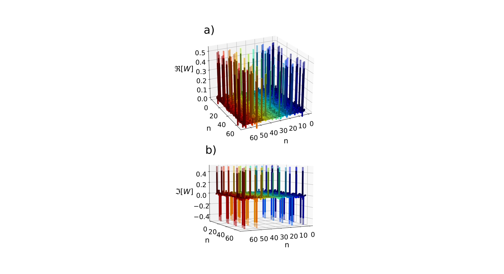
To further assess the agreement between our experiment and theory, we estimate the fidelity of the measured process matrix $W_{\text{exp}}$ to the ideal matrix $W_{s}^{y-}$. Since every valid process matrix normalized by its trace is a valid quantum state, we use the conventional expression for calculating the fidelity $F(\sigma,\rho)=\Tr\big(\sqrt{\sqrt{\sigma}\rho\sqrt{\sigma}}\big)$ with $\sigma$ and $\rho$ being different density matrices Nielsen and Chuang 2005. This results in a fidelity of

where the error arises is estimated using a Monte Carlo simulation of the entire reconstruction procedure accounting for finite measurement statistics and small waveplate errors of $1^{\circ}$. Especially given the high-dimension of our process matrix, this fidelity indicates that our experiment is quite close to theory.

To quantify the agreement between our experimental data and $W_{\text{exp}}$ we compare the residuals of our fit $r$ (defined in Eq. 29) to the average statistical error of our data $\eta_{\text{stat}}$. The residuals $r$ can be interpreted as the disagreement between the outcome predicted by $W_{\text{exp}}$ and the measured experimental outcome, averaged over all measurement settings. For our fit $r=0.0089$, indicating an excellent match to our experimental data. We estimate our statistical errors as follows. First, we treat the probability to obtain an outcome $abc$ as a binomial variable: either we detect a photon or we do not. Then we estimate the variance of that setting as $N_{xyzw}\penalty\ p(abc|xyzw)\times(1-p(abc|xyzw))$, where $N_{xyzw}$ is the number of photons detected in all outcomes associated with $xyzw$ (defined in Eq. 31). Finally, we compute the average error per setting as

This is simply the standard error of each setting operator averaged over all settings. Evaluating this for our data, we find $\eta_{\text{stat}}=0.0056$. Given that $\eta_{\text{stat}}\approx r$, we conclude that our process matrix fits our data well.

A bipartite process matrix without a common past is causally non-separable when it cannot be written as a classical mixture of causally ordered processes Oreshkov et al. 2012; Araújo et al. 2015. When considering bipartite processes with a common past, such as the quantum switch considered in this work, there are different non-equivalent definitions of indefinite causality. In Ref. Araújo et al. 2015; Rubino et al. 2017, a bipartite process matrix $W\in\penalty\ \mathcal{L}\left(\mathcal{H}_{P}\otimes\mathcal{H}_{A_{\text{in}}}\otimes\mathcal{H}_{A_{\text{out}}}\otimes\mathcal{H}_{B_{\text{in}}}\otimes\mathcal{H}_{B_{\text{out}}}\otimes\mathcal{H}_{F}\right)$ with common past and common future is said to be causally separable if it can be written as a convex sum of causally-ordered process matrices. That is, if we can write

where $p\in[0,1]$, and $W^{A>B}$ and $W^{B>A}$ are causally-ordered process (objects also referred to as quantum combs Chiribella et al. 2009; Chiribella et al. 2013, see Appendix C). Alternatively, Ref. Oreshkov and Giarmatzi 2016 proposes the concept of extensible causally-separable processes. This leads to a definition which differs from the one in Eq. (35), but is equivalent to the definition of causal-separability presented in Ref. Wechs et al. 2019, which considers not only convex mixtures of causally-ordered processes, but also incoherent (hence, classical) control of causal order. The analysis and the numbers presented in this section and in the main part of this paper were obtained via the definition of Rubino et al. 2017, which is the one presented in Eq. (35). However, we stress that the results of our work are not qualitatively affected by the different before-mentioned definitions, in the sense that, in all cases, the process we obtain after tomography is not causally separable, and it is robust against different kinds of noise. In Appendix C, we present a more detailed discussion of such definitions and how they make small quantitative changes in the numbers presented here.

One method to quantify the degree to which our quantum process is causally non-separable is by using a causal witness. A causal witness is a Hermitian non-negative operator ${G}$ such that $\Tr\left({G}W_{\text{sep}}\right)\geq 0$ for all causally-separable processes. However, for all causally–non-separable processes (such as the quantum SWITCH) one can always find a witness ${G}$ such that $\Tr\left({G}W^{y-}_{s}\right)<\penalty\ 0$. Without additional constraints, the quantity $\Tr\left({G}W\right)$ does not have a physical meaning, and may be artificially inflated by multiplying the witness $G$ by some constant. However, by setting additional normalisation constraints on the witness $G$, one may identify the quantity $\Tr\left({G}W\right)$ with how much noise the process $W$ can tolerate until it becomes causality separable. More concretely, let $\mathds{1}_{W}:=\frac{\mathds{1}}{d_{P}d_{A_{O}}d_{B_{O}}}$ be the “white noise process”, which simply consists of discarding everything and outputting white noise, and let $W_{\text{sep}}$ be an arbitrary causally-separable process matrix. Ref. Araújo et al. 2015 shows that the problem

is equivalent to its dual formulation

Hence, under the normalisation constraint $\Tr(G)\leq\penalty\ \Tr(\id_W)$, we ensure the identity $\Tr(G W)=-r$, which allows us to interpret $\Tr(G W)$ as how robust $W$ is against white noise.

Alternatively, one may also consider the normalisation $\Tr(G \Omega)\leq 1$, where $\Omega$ is an arbitrary process matrix. In this case, the equivalent problem reads as

where $\Omega$ is an arbitrary process matrix. In this case, the value $\Tr(GW)=-r$ is typically called the “generalised robustness”; it may be viewed as the amount of noise one needs to add to $W$ to make it causally separable in the worst case scenario.

In order for the witness $G$ to fit the setting operators implemented in our experiment, we impose an additional structure on the witness $G$ which is given by

where $\alpha_{a,b,c,x,y,z,w}$ are arbitrary real numbers and $S_{abc|xyzw}$ are the setting operators of our experiment (see Sec. II.5). Additionally, for fixed setting operators, finding the maximal violation of a witness $G$ with the normalization constraints related to white and generalised noise is a Semidefinite Program (SDP) Araújo et al. 2015, and can be efficiently solved numerically Boyd and Vandenberghe 2004. Our code doing so is also available at Antesberger et al. 2023.

With these tools, we can construct a variety of witnesses. First, we can construct witnesses using the complete measurement set (Eq. 28) or our restricted measurement set (Eq. 77). We can further design witnesses for two different process matrices $W^{y-}_{s}$ or $W_{\text{exp}}$. This results in four witnesses: ${G}_{\text{y-,all}}$, ${G}_{\text{y-, res}}$, ${G}_{\text{exp,all}}$, ${G}_{\text{exp, res}}$. Where the subscript $y-$ (exp) indicates that the witness was optimized for the ideal (experimental) process matrix, and the subscript all (res) indicates that the witness was computed using the complete (restricted) measurement set. We can then further construct witness for either the generalized or white noise robustness.

The results of the generalized robustness witnesses are summarized in Tab. 1. The first row of Tab. 1 shows the value of the four witnesses evaluated using $W^{y-}_{s}$, and the second row shows the experimental values, estimated using $W_{\text{exp}}$. In this case, we see that $\Tr(W^{y-}G_\text{y-,res}^\text{GR})\approx\penalty\ \Tr(W^{y-}G_\text{y-,all}^\text{GR})$ and $\Tr(W^\text{exp}G_\text{exp,res}^\text{GR})\approx\penalty\ \Tr(W^\text{exp}G_\text{exp,all}^\text{GR})$. In other words, the generalized robustness evaluated either with the complete or restricted setting operators is equal within experimental error. Evidently, the additional measurement on the future control system does not affect the generalized robustness. More interesting for the generalized robustness witnesses, is the performance of the witnesses optimized for our experimental process matrix $W_{\text{exp}}$. Examining the performance of our experimentally estimated witnesses (the bottom row of Tab. 1), we see that the witnesses designed specifically for our experimental process matrix increase the generalized robustness. In particular, $\Tr(W_\text{exp}G_\text{exp,all}^\text{GR})>\penalty\ \Tr(W_\text{exp}G_\text{y-,all}^\text{GR})$ and $\Tr(W_\text{exp}G_\text{exp,res}^\text{GR})>\penalty\ \Tr(W_\text{exp}G_\text{y-,res}^\text{GR})$. This would not be readily possible without performing process matrix tomography.

In Tab. 2 we summarize the results of our white noise witness analysis. In this case, we see a significant difference between the witnesses constructed with the restricted and complete measurement sets, with the complete measurements sets revealing a higher white noise robustness in all cases. Furthermore, in the second row, we can see that each step progressively improves the experimental white noise robustness. The first entry $\Tr(G_\text{y-,res}^\text{WN} W_\text{exp})=-1.65\pm 0.02$ shows the value that one would obtain for our setup without performing process matrix tomography. i.e. the witness was designed for the ideal process and uses only the experimentally implementable measurement settings. In the next column, $\Tr(G_\text{exp,res}^\text{WN} W_\text{exp})=-1.76\pm 0.01$ is improved by tailoring the witness for our experiment; however, still using only experimentally implementable measurements. In the next two columns, we improve both of these values further by computing the witness assuming the complete measurement set. The final entry, $\Tr(G_\text{exp,all}^\text{WN} W_\text{exp})=-2.11\pm 0.02$ is significantly higher than the first entry, clearly showing the power of full process matrix tomography. Process matrix tomography allows us to compute properties of the experimental process, without having direct experimental access to them and we can precisely tailor our analysis to our experimental conditions. In the Appendix tables 3 and 4, we show the same analysis, for the alternative definition of causal non-separability. The trends observed therein are the same, although the absolute values of the robustnesses are smaller.

For the process tomography results presented in Sec. IV.1, we found the process matrix that fit to our data best, by minimizing Eq. 29. As discussed there, this resulted in a process matrix that describes our data very well. However, one could ask “Are there other causally-separable process matrices that describe the data almost as well?” To answer this question, we perform a “worst-case” version of our process matrix tomography. To do so, rather than minimizing expression Eq. 29, we find the process matrix that maximizes the generalized or white noise robustness, $\Tr(W_\text{worst} {G}_\text{j,all}^\text{GR})$ or $\Tr(W_\text{worst} {G}_\text{j,all}^\text{WN})$, respectively. We do this using the witnesses designed for the ideal process matrix and the originally reconstructed experimental process matrix, but always with the complete measurement sets. This maximisation is subject to the constraints that $W_{\text{worst}}$ is a physical process matrix and that the predictions of $W_{\text{worst}}$ match the experiment within some error $\epsilon$:

Here $\epsilon$ is closely related to the residuals defined in Eq. 29. In particular, if $\epsilon<r$ the maximization will fail, as there is no physical process matrix compatible with this constraint. Thus, we perform worst case process tomography for the four witnesses discussed above starting from $\epsilon=r_{\text{exp}}=0.0089$ and increasing to $\epsilon=0.015$. The results of this analysis are plotted in Fig. 7a and b. We find that the generalized robustness witnesses are more tolerant $\epsilon$, finding that our data is only consistent with causally separable process matrices for $\epsilon\lesssim 0.012$, while the white noise witnesses require $\epsilon\lesssim 0.0105$. Although this analysis suggests that the causal non-separability is rather fragile, we stress the worst-case nature of this treatment: if a single causally separable process matrix is compatible to our data within $\epsilon$ it will be returned, even if a causally non-separable data fits our data better. In any case, we see that for a range of experimentally relevant errors our data are only compatible with a causally non-separable process matrix.

References

- Selinger and Valiron (2009) P. Selinger and B. Valiron, Quantum lambda calculus, in Semantic Techniques in Quantum Computation, edited by S. Gay and I. Mackie (Cambridge University Press, 2009) p. 135–172.
- Chiribella et al. (2008) G. Chiribella, G. M. D’Ariano, and P. Perinotti, Quantum Circuit Architecture, Phys. Rev. Lett. 101, 060401 (2008), arXiv:0712.1325 [quant-ph] .
- Gutoski and Watrous (2007) G. Gutoski and J. Watrous, Toward a general theory of quantum games, in Proceedings of the thirty-ninth annual ACM symposium on Theory of computing (2007) pp. 565–574, quant-ph/0611234 .
- Chiribella et al. (2009) G. Chiribella, G. M. D’Ariano, and P. Perinotti, Theoretical framework for quantum networks, Phys. Rev. A 80, 022339 (2009), arXiv:0904.4483 [quant-ph] .
- Bisio and Perinotti (2019) A. Bisio and P. Perinotti, Theoretical framework for higher-order quantum theory, Proceedings of the Royal Society of London Series A 475, 20180706 (2019), arXiv:1806.09554 [quant-ph] .
- Oreshkov et al. (2012) O. Oreshkov, F. Costa, and Č. Brukner, Quantum correlations with no causal order, Nature Communications 3, 1092 (2012), arXiv:1105.4464 [quant-ph] .
- Hardy (2007) L. Hardy, Towards quantum gravity: a framework for probabilistic theories with non-fixed causal structure, Journal of Physics A Mathematical General 40, 3081 (2007), arXiv:gr-qc/0608043 [gr-qc] .
- Chiribella et al. (2013) G. Chiribella, G. M. D’Ariano, P. Perinotti, and B. Valiron, Quantum computations without definite causal structure, Phys. Rev. A 88, 022318 (2013), arXiv:0912.0195 [quant-ph] .
- Brukner (2014) Č. Brukner, Quantum causality, Nature Physics 10, 259 (2014).
- Baumeler and Wolf (2014) Ä. Baumeler and S. Wolf, Perfect signaling among three parties violating predefined causal order, in 2014 IEEE International Symposium on Information Theory (IEEE, 2014) pp. 526–530, arXiv:1312.5916 [quant-ph] .
- Oreshkov and Giarmatzi (2016) O. Oreshkov and C. Giarmatzi, Causal and causally separable processes, New Journal of Physics 18, 093020 (2016), arXiv:1506.05449 [quant-ph] .
- Baumeler and Wolf (2016) Ä. Baumeler and S. Wolf, The space of logically consistent classical processes without causal order, New Journal of Physics 18, 013036 (2016), arXiv:1507.01714 [quant-ph] .
- Araújo et al. (2015) M. Araújo, C. Branciard, F. Costa, A. Feix, C. Giarmatzi, and Č. Brukner, Witnessing causal nonseparability, New Journal of Physics 17, 102001 (2015), arXiv:1506.03776 [quant-ph] .
- Branciard (2016) C. Branciard, Witnesses of causal nonseparability: an introduction and a few case studies, Scientific Reports 6, 26018 (2016), arXiv:1603.00043 [quant-ph] .
- Zych et al. (2019) M. Zych, F. Costa, I. Pikovski, and Č. Brukner, Bell’s theorem for temporal order, Nature communications 10, 1 (2019).
- Hardy (2009) L. Hardy, Quantum gravity computers: On the theory of computation with indefinite causal structure, in Quantum reality, relativistic causality, and closing the epistemic circle (Springer, 2009) pp. 379–401.
- Araújo et al. (2014) M. Araújo, F. Costa, and Č. Brukner, Computational Advantage from Quantum-Controlled Ordering of Gates, Phys. Rev. Lett. 113, 250402 (2014), arXiv:1401.8127 [quant-ph] .
- Araújo et al. (2017) M. Araújo, P. A. Guérin, and ń. Baumeler, Quantum computation with indefinite causal structures, Phys. Rev. A 96, 052315 (2017), arXiv:1706.09854 [quant-ph] .
- Renner and Brukner (2022) M. J. Renner and Č. Brukner, Computational Advantage from a Quantum Superposition of Qubit Gate Orders, Phys. Rev. Lett. 128, 230503 (2022), arXiv:2112.14541 [quant-ph] .
- Feix et al. (2015) A. Feix, M. Araújo, and Č. Brukner, Quantum superposition of the order of parties as a communication resource, Phys. Rev. A 92, 052326 (2015), arXiv:1508.07840 [quant-ph] .
- Guérin et al. (2016) P. A. Guérin, A. Feix, M. Araújo, and Č. Brukner, Exponential communication complexity advantage from quantum superposition of the direction of communication, Phys. Rev. Lett. 117, 100502 (2016), arXiv:1605.07372 [quant-ph] .
- Ebler et al. (2018) D. Ebler, S. Salek, and G. Chiribella, Enhanced Communication with the Assistance of Indefinite Causal Order, Phys. Rev. Lett. 120, 120502 (2018), arXiv:1711.10165 [quant-ph] .
- Jia and Costa (2019) D. Jia and F. Costa, Causal order as a resource for quantum communication, Phys. Rev. A 100, 052319 (2019), arXiv:1901.09159 [quant-ph] .
- Kristjánsson et al. (2020) H. Kristjánsson, G. Chiribella, S. Salek, D. Ebler, and M. Wilson, Resource theories of communication, New Journal of Physics 22, 073014 (2020), arXiv:1910.08197 [quant-ph] .
- Chiribella and Kristjánsson (2019) G. Chiribella and H. Kristjánsson, Quantum Shannon theory with superpositions of trajectories, Proceedings of the Royal Society of London Series A 475, 20180903 (2019), arXiv:1812.05292 [quant-ph] .
- Chiribella et al. (2021) G. Chiribella, M. Banik, S. S. Bhattacharya, T. Guha, M. Alimuddin, A. Roy, S. Saha, S. Agrawal, and G. Kar, Indefinite causal order enables perfect quantum communication with zero capacity channels, New Journal of Physics 23, 033039 (2021), arXiv:1810.10457 [quant-ph] .
- Caleffi and Cacciapuoti (2020) M. Caleffi and A. S. Cacciapuoti, Quantum switch for the quantum internet: Noiseless communications through noisy channels, IEEE Journal on Selected Areas in Communications 38, 575 (2020).
- Procopio et al. (2020) L. M. Procopio, F. Delgado, M. Enríquez, N. Belabas, and J. A. Levenson, Sending classical information via three noisy channels in superposition of causal orders, Phys. Rev. A 101, 012346 (2020), arXiv:1910.11137 [quant-ph] .
- Chiribella (2012) G. Chiribella, Perfect discrimination of no-signalling channels via quantum superposition of causal structures, Phys. Rev. A 86, 040301 (2012), arXiv:1109.5154 [quant-ph] .
- Bavaresco et al. (2021) J. Bavaresco, M. Murao, and M. T. Quintino, Strict hierarchy between parallel, sequential, and indefinite-causal-order strategies for channel discrimination, Phys. Rev. Lett. 127, 200504 (2021), arXiv:2011.08300 [quant-ph] .
- Zhao et al. (2020) X. Zhao, Y. Yang, and G. Chiribella, Quantum Metrology with Indefinite Causal Order, Phys. Rev. Lett. 124, 190503 (2020), arXiv:1912.02449 [quant-ph] .
- Quintino et al. (2019) M. T. Quintino, Q. Dong, A. Shimbo, A. Soeda, and M. Murao, Reversing Unknown Quantum Transformations: Universal Quantum Circuit for Inverting General Unitary Operations, Phys. Rev. Lett. 123, 210502 (2019), arXiv:1810.06944 [quant-ph] .
- Schiansky et al. (2023) P. Schiansky, T. Strömberg, D. Trillo, V. Saggio, B. Dive, M. Navascués, and P. Walther, Demonstration of universal time-reversal for qubit processes, Optica 10, 200 (2023), arXiv:2205.01122 [quant-ph] .
- Felce and Vedral (2020) D. Felce and V. Vedral, Quantum Refrigeration with Indefinite Causal Order, Phys. Rev. Lett. 125, 070603 (2020), arXiv:2003.00794 [quant-ph] .
- Procopio et al. (2015) L. M. Procopio, A. Moqanaki, M. Araújo, F. Costa, I. Alonso Calafell, E. G. Dowd, D. R. Hamel, L. A. Rozema, Č. Brukner, and P. Walther, Experimental superposition of orders of quantum gates, Nature Communications 6, 7913 (2015), arXiv:1412.4006 [quant-ph] .
- Goswami et al. (2020) K. Goswami, Y. Cao, G. A. Paz-Silva, J. Romero, and A. G. White, Increasing communication capacity via superposition of order, Phys. Rev. Research 2, 033292 (2020).
- Wei et al. (2019) K. Wei, N. Tischler, S.-R. Zhao, Y.-H. Li, J. M. Arrazola, Y. Liu, W. Zhang, H. Li, L. You, Z. Wang, Y.-A. Chen, B. C. Sanders, Q. Zhang, G. J. Pryde, F. Xu, and J.-W. Pan, Experimental Quantum Switching for Exponentially Superior Quantum Communication Complexity, Phys. Rev. Lett. 122, 120504 (2019), arXiv:1810.10238 [quant-ph] .
- Guo et al. (2020) Y. Guo, X.-M. Hu, Z.-B. Hou, H. Cao, J.-M. Cui, B.-H. Liu, Y.-F. Huang, C.-F. Li, G.-C. Guo, and G. Chiribella, Experimental transmission of quantum information using a superposition of causal orders, Phys. Rev. Lett. 124, 030502 (2020), arXiv:1811.07526 [quant-ph] .
- Rubino et al. (2021) G. Rubino, L. A. Rozema, D. Ebler, H. Kristjánsson, S. Salek, P. Allard Guérin, A. A. Abbott, C. Branciard, Č. Brukner, G. Chiribella, and P. Walther, Experimental quantum communication enhancement by superposing trajectories, Physical Review Research 3, 013093 (2021), arXiv:2007.05005 [quant-ph] .
- Taddei et al. (2021) M. M. Taddei, J. Cariñe, D. Martínez, T. García, N. Guerrero, A. A. Abbott, M. Araújo, C. Branciard, E. S. Gómez, S. P. Walborn, L. Aolita, and G. Lima, Computational advantage from the quantum superposition of multiple temporal orders of photonic gates, PRX Quantum 2, 010320 (2021), arXiv:2002.07817 [quant-ph] .
- Pang et al. (2023) A. O. Pang, N. Lupu-Gladstein, H. Ferretti, Y. B. Yilmaz, A. Brodutch, and A. M. Steinberg, Experimental communication through superposition of quantum channels, arXiv preprint arXiv:2302.14820 10.48550/arXiv.2302.14820 (2023).
- Liu et al. (2023) W.-Q. Liu, Z. Meng, B.-W. Song, J. Li, Q.-Y. Wu, X.-X. Chen, J.-Y. Hong, A.-N. Zhang, and Z.-q. Yin, Experimentally demonstrating indefinite causal order algorithms to solve the generalized Deutsch’s problem, arXiv e-prints (2023), arXiv:2305.05416 [quant-ph] .
- Rubino et al. (2017) G. Rubino, L. A. Rozema, A. Feix, M. Araújo, J. M. Zeuner, L. M. Procopio, Č. Brukner, and P. Walther, Experimental verification of an indefinite causal order, Science Advances 3, e1602589 (2017), arXiv:1608.01683 [quant-ph] .
- Goswami et al. (2018) K. Goswami, C. Giarmatzi, M. Kewming, F. Costa, C. Branciard, J. Romero, and A. G. White, Indefinite causal order in a quantum switch, Phys. Rev. Lett. 121, 090503 (2018).
- Rubino et al. (2022) G. Rubino, L. A. Rozema, F. Massa, M. Araújo, M. Zych, Č. Brukner, and P. Walther, Experimental entanglement of temporal order, Quantum 6, 621 (2022), arXiv:1712.06884 [quant-ph] .
- Cao et al. (2023) H. Cao, J. Bavaresco, N.-N. Wang, L. A. Rozema, C. Zhang, Y.-F. Huang, B.-H. Liu, C.-F. Li, G.-C. Guo, and P. Walther, Semi-device-independent certification of indefinite causal order in a photonic quantum switch, Optica 10, 561 (2023), arXiv:2202.05346 [quant-ph] .
- Rambo et al. (2016) T. M. Rambo, J. B. Altepeter, P. Kumar, and G. M. D’Ariano, Functional quantum computing: An optical approach, Phys. Rev. A 93, 052321 (2016), arXiv:1211.1257 [quant-ph] .
- Chiribella and Liu (2022) G. Chiribella and Z. Liu, Quantum operations with indefinite time direction, Communications Physics 5, 190 (2022), arXiv:2012.03859 [quant-ph] .
- Guo et al. (2022) Y. Guo, Z. Liu, H. Tang, X.-M. Hu, B.-H. Liu, Y.-F. Huang, C.-F. Li, G.-C. Guo, and G. Chiribella, Experimental demonstration of input-output indefiniteness in a single quantum device, arXiv e-prints (2022), arXiv:2210.17046 [quant-ph] .
- Strömberg et al. (2022a) T. Strömberg, P. Schiansky, M. Túlio Quintino, M. Antesberger, L. Rozema, I. Agresti, Č. Brukner, and P. Walther, Experimental superposition of time directions, arXiv e-prints (2022a), arXiv:2211.01283 [quant-ph] .
- Strömberg et al. (2022b) T. Strömberg, P. Schiansky, R. W. Peterson, M. Túlio Quintino, and P. Walther, Demonstration of a quantum SWITCH in a Sagnac configuration, arXiv e-prints (2022b), arXiv:2211.12540 [quant-ph] .
- Paunković and Vojinović (2020) N. Paunković and M. Vojinović, Causal orders, quantum circuits and spacetime: distinguishing between definite and superposed causal orders, Quantum 4, 275 (2020), arXiv:1905.09682 [quant-ph] .
- Vilasini and Renner (2022) V. Vilasini and R. Renner, Embedding cyclic causal structures in acyclic spacetimes: no-go results for process matrices, arXiv preprint (2022), arXiv:2203.11245 [quant-ph] .
- Ormrod et al. (2022) N. Ormrod, A. Vanrietvelde, and J. Barrett, Causal structure in the presence of sectorial constraints, with application to the quantum switch, arXiv preprint (2022), arXiv:2204.10273 [quant-ph] .
- Oreshkov (2019) O. Oreshkov, Time-delocalized quantum subsystems and operations: on the existence of processes with indefinite causal structure in quantum mechanics, Quantum 3, 206 (2019), arXiv:1801.07594 [quant-ph] .
- de la Hamette et al. (2022) A.-C. de la Hamette, V. Kabel, M. Christodoulou, and Č. Brukner, Quantum diffeomorphisms cannot make indefinite causal order definite, arXiv e-prints (2022), arXiv:2211.15685 [quant-ph] .
- Fellous-Asiani et al. (2023) M. Fellous-Asiani, R. Mothe, L. Bresque, H. Dourdent, P. A. Camati, A. A. Abbott, A. Auffèves, and C. Branciard, Comparing the quantum switch and its simulations with energetically constrained operations, Physical Review Research 5 (2023), arXiv:2208.01952 [quant-ph] .
- Gühne and Tóth (2009) O. Gühne and G. Tóth, Entanglement detection, Physics Reports 474, 1 (2009).
- Bavaresco et al. (2019) J. Bavaresco, M. Araújo, Č. Brukner, and M. T. Quintino, Semi-device-independent certification of indefinite causal order, Quantum 3, 176 (2019), arXiv:1903.10526 [quant-ph] .
- Dourdent et al. (2022) H. Dourdent, A. A. Abbott, N. Brunner, I. Šupić, and C. Branciard, Semi-Device-Independent Certification of Causal Nonseparability with Trusted Quantum Inputs, Phys. Rev. Lett. 129, 090402 (2022), arXiv:2107.10877 [quant-ph] .
- van der Lugt et al. (2022) T. van der Lugt, J. Barrett, and G. Chiribella, Device-independent certification of indefinite causal order in the quantum switch, arXiv e-prints (2022), arXiv:2208.00719 [quant-ph] .
- Gogioso and Pinzani (2022a) S. Gogioso and N. Pinzani, The Topology and Geometry of Causality, arXiv e-prints (2022a), arXiv:2206.08911 [quant-ph] .
- Ziman (2008) M. Ziman, Process positive-operator-valued measure: A mathematical framework for the description of process tomography experiments, Phys. Rev. A 77, 062112 (2008), arXiv:0802.3862 [quant-ph] .
- Chuang and Nielsen (1997) I. L. Chuang and M. A. Nielsen, Prescription for experimental determination of the dynamics of a quantum black box, Journal of Modern Optics 44, 2455 (1997).
- Poyatos et al. (1997) J. Poyatos, J. I. Cirac, and P. Zoller, Complete characterization of a quantum process: the two-bit quantum gate, Phys. Rev. Lett. 78, 390 (1997).
- O’Brien et al. (2004) J. L. O’Brien, G. J. Pryde, A. Gilchrist, D. F. James, N. K. Langford, T. C. Ralph, and A. G. White, Quantum process tomography of a controlled-not gate, Phys. Rev. Lett. 93, 080502 (2004).
- Bisio et al. (2017) A. Bisio, G. Chiribella, G. Mauro D’Ariano, S. Facchini, and P. Perinotti, Optimal quantum tomography, arXiv e-prints , arXiv:1702.08751 (2017), arXiv:1702.08751 [quant-ph] .
- Mohseni et al. (2008) M. Mohseni, A. T. Rezakhani, and D. A. Lidar, Quantum-process tomography: Resource analysis of different strategies, Phys. Rev. A 77, 032322 (2008), arXiv:quant-ph/0702131 [quant-ph] .
- Rozema et al. (2014) L. A. Rozema, D. H. Mahler, R. Blume-Kohout, and A. M. Steinberg, Optimizing the choice of spin-squeezed states for detecting and characterizing quantum processes, Physical Review X 4, 041025 (2014), arXiv:1405.5444 [quant-ph] .
- Nielsen and Chuang (2005) M. A. Nielsen and I. L. Chuang, Quantum computation and quantum information, 8th ed. (Cambridge Univ. Press, Cambridge [u.a.], 2005).
- Bisio et al. (2010) A. Bisio, G. Chiribella, G. M. D’Ariano, S. Facchini, and P. Perinotti, Optimal quantum learning of a unitary transformation, Phys. Rev. A 81, 032324 (2010), arXiv:0903.0543 [quant-ph] .
- Sedlák et al. (2019) M. Sedlák, A. Bisio, and M. Ziman, Optimal Probabilistic Storage and Retrieval of Unitary Channels, Phys. Rev. Lett. 122, 170502 (2019), arXiv:1809.04552 [quant-ph] .
- Bavaresco et al. (2022) J. Bavaresco, M. Murao, and M. T. Quintino, Unitary channel discrimination beyond group structures: Advantages of sequential and indefinite-causal-order strategies, Journal of Mathematical Physics 63, 042203 (2022), arXiv:2105.13369 [quant-ph] .
- Jamiołkowski (1972) A. Jamiołkowski, Linear transformations which preserve trace and positive semidefiniteness of operators, Reports on Mathematical Physics 3, 275 (1972).
- Choi (1975) M.-D. Choi, Completely positive linear maps on complex matrices, Linear algebra and its applications 10, 285 (1975).
- Gogioso and Pinzani (2022b) S. Gogioso and N. Pinzani, The Topology and Geometry of Causality, arXiv e-prints , arXiv:2206.08911 (2022b), arXiv:2206.08911 [quant-ph] .
- Wootters (1990) W. K. Wootters, Local accessibility of quantum states, Complexity, entropy and the physics of information, edited by W. H. Zurek (Addison-Wesley, Reading, MA, 1990), pp. 39–46. 8, 39 (1990).
- de Burgh et al. (2008) M. D. de Burgh, N. K. Langford, A. C. Doherty, and A. Gilchrist, Choice of measurement sets in qubit tomography, Phys. Rev. A 78, 052122 (2008).
- Antesberger et al. (2023) M. Antesberger, M. T. Quintino, P. Walther, and L. A. Rozema, Raw data and analysis code for "Higher-order Process Matrix Tomography of a passively-stable Quantum SWITCH", 10.5281/zenodo.7974799 (2023).
- Vedovato et al. (2018) F. Vedovato, C. Agnesi, M. Tomasin, M. Avesani, J.-Å. Larsson, G. Vallone, and P. Villoresi, Postselection-Loophole-Free Bell Violation with Genuine Time-Bin Entanglement, Phys. Rev. Lett. 121, 190401 (2018), arXiv:1804.10150 [quant-ph] .
- Zanin et al. (2021) G. L. Zanin, M. J. Jacquet, M. Spagnolo, P. Schiansky, I. A. Calafell, L. A. Rozema, and P. Walther, Fiber-compatible photonic feed-forward with 99% fidelity, Opt. Express 29, 3425 (2021), arXiv:2009.07868 [quant-ph] .
- Zanin et al. (2022) G. L. Zanin, M. Antesberger, M. J. Jacquet, P. H. S. Ribeiro, L. A. Rozema, and P. Walther, Enhanced Photonic Maxwell’s Demon with Correlated Baths, Quantum 6, 810 (2022), arXiv:2107.09686 [quant-ph] .
- Kim et al. (2006) T. Kim, M. Fiorentino, and F. N. C. Wong, Phase-stable source of polarization-entangled photons using a polarization Sagnac interferometer, Phys. Rev. A 73, 012316 (2006), arXiv:quant-ph/0509219 [quant-ph] .
- Wechs et al. (2019) J. Wechs, A. A. Abbott, and C. Branciard, On the definition and characterisation of multipartite causal (non)separability, New Journal of Physics 21, 013027 (2019), arXiv:1807.10557 [quant-ph] .
- Boyd and Vandenberghe (2004) S. Boyd and L. Vandenberghe, Convex Optimization (Cambridge University Press, 2004).
- Flammia et al. (2012) S. T. Flammia, D. Gross, Y.-K. Liu, and J. Eisert, Quantum tomography via compressed sensing: error bounds, sample complexity and efficient estimators, New Journal of Physics 14, 095022 (2012), arXiv:1205.2300 [quant-ph] .
- Aaronson (2020) S. Aaronson, Shadow tomography of quantum states (2020) pp. STOC18–368–STOC18–394, arXiv:1711.01053 [quant-ph] .
- Mahler et al. (2013) D. H. Mahler, L. A. Rozema, A. Darabi, C. Ferrie, R. Blume-Kohout, and A. M. Steinberg, Adaptive Quantum State Tomography Improves Accuracy Quadratically, Phys. Rev. Lett. 111, 183601 (2013), arXiv:1303.0436 [quant-ph] .
Appendix A Experimental techniques
In this section, the used SPDC photon pair source is described and the technique implemented to compensate for unwanted polarization transformations induced by the birefringence of the optical fibers is explained. Moreover, the implemented experimental instruments and measurements are shown in detail.
A.1 Photon Source
To generate photon pairs at a wavelength of nm we use a 775 nm, CW laser beam to pump a 30mm long ppKTP crystal. A dichroic mirror reflects 775 nm light and transmits photons at 1550 nm. The signal and idler photon are then separated on a PBS and coupled over optical fibers into the setup.
A.2 Polarization Compensation
In order to ensure that the quantum SWITCH performs the desired transformations on the photon’s polarization, it is important to correct for the birefringent behaviour of the fibers that connect Alice and Bob’s laboratories; i.e. to ensure that the fibers do not change the polarization state of the photon. Hence, each fiber link has to perform an identity operation. To this end, each fiber is equipped with a 3-loop fiber polarization controller, which allows us to implement any unitary polarization transformation in the fiber. In order to implement a true identity operation, we must check that the correct transformation is applied in two different bases. We use the computational and diagonal bases. A convenient way to do this, is to send classical light at the same wavelength as the single photons through the fibers and detect the polarization with a polarimeter at the fiber output. To ensure the identity transformation, we switch the light’s polarization state at the target preparation stage(see Fig. 4) between horizontal and diagonal , while adjusting the polarization controller until it converges to the correct setting in both bases. To correct the polarization for the second trip through the channels, we place a polarizer in one of the channels (without additional waveplates). This decouples the compensation from the previous fiber. Then, we follow the same procedure and alternate the polarizer to transmit and then . In order for this procedure to work properly, it is essential that wavelengths of the classical light and the single photons is matched.
A.3 Experimental Instruments and Measurements
Here we explain in detail the measurements and instruments we implement in the lab, and how they relate the ideal settings discussed in the main text.
A.3.1 Future Control Measurement
Our control qubit is the time-bin qubit. Its past state is fixed to . Ideally, we would measure the future control in three different bases described by Eqs. 21 - 23. However, due to experimental limitations we only measure the future control in two bases