Modeling and testing screening mechanisms in the laboratory and in space
Abstract
The non-linear dynamics of scalar fields coupled to matter and gravity can lead to remarkable density-dependent screening effects. In this short review we present the main classes of screening mechanisms, and discuss their tests in laboratory and astrophysical systems. We particularly focus on reviewing numerical and technical aspects involved in modeling the non-linear dynamics of screening. In this review, we focus on tests using laboratory experiments and astrophysical systems, such as stars, galaxies and dark matter halos.
keywords
Modified Gravity; Screening Mechanisms; Laboratory Tests of Gravity, Astrophysical Tests of Gravity2 Center for Data-Driven Discovery, Kavli IPMU (WPI), UTIAS, The University of Tokyo, Kashiwa, Chiba 277-8583, Japan
3 CNRS & Sorbonne Université, Institut d’Astrophysique de Paris (IAP), UMR 7095, 98 bis bd Arago, F-75014 Paris, France
††corresponding: Correspondence: valeri.vardanyan@ipmu.jp (V.V.); deaglan.bartlett@iap.fr (D.J.B.)††reftitle: References
1 Introduction
The accelerated expansion of the Universe, discovered over two decades ago Perlmutter et al. 1999; Riess et al. 1998, still lacks a satisfactory theoretical explanation. Scalar fields have played a significant role in modeling cosmic acceleration, and provide a relatively simple playground for establishing novel phenomenological features. Such scalar fields have been considered in two broad contexts, namely, Dark Energy (see e.g. Ref. Copeland et al. 2006) and modifications of Einstein’s General Relativity (GR) (see e.g. Refs. Silvestri and Trodden 2009; Clifton et al. 2012; Joyce et al. 2015; Koyama 2016). The defining feature of modified gravity theories is the non-trivial coupling of scalar fields to gravity and matter. In modified gravity, therefore, one expects long-range “fifth” forces across a very broad range of scales, manifesting themselves from microscopically small scales to cosmologically large ones, characterized by the present-day expansion rate .
In the cosmological regime, the phenomenology can be well-understood with linear perturbation theory methods. Particularly, the primary modifications are expressed as scale-and-time-dependent gravitational coupling and lensing potential (see e.g. Refs. Ade et al. 2016; Pogosian and Silvestri 2016). Ongoing and upcoming large scale structure surveys are the primary testing ground for cosmological phenomenology of modified gravity. However, in order to have consistent dynamics on all the scales of interest, fifth forces should be screened away in regions much denser than the mean cosmological environments. Otherwise, such fifth forces would be ruled out on the grounds of local tests of gravity, which provide stringent constraints on additional interactions Will 1993.
The inherently non-linear dynamics of non-trivially coupled scalar fields can lead to remarkably diverse effects depending on the environment where they operate. Particularly, it has been realized that non-minimally coupled scalar fields with or without higher-derivative terms can lead to the so-called screening effects in dense environments. This environmental dependence allows the field to induce large deviations from GR on relatively poorly constrained cosmological structure formation and gravitational lensing scales, while having smaller effects in regimes where GR has been tested more precisely.
The most widely considered working scenario, known as chameleon mechanism, has been proposed and investigated in Refs. Khoury and Weltman 2004a; Khoury and Weltman 2004b; Brax et al. 2004. A related scenario is the so called symmetron screening, introduced and studied in Refs. Hinterbichler and Khoury 2010; Hinterbichler et al. 2011. Both of these classes operate due to non-linearities in the potential sector. Non-linearities in the derivative sector can also lead to density-dependent screening, for example, the Vainshtein mechanism Vainshtein 1972; Nicolis et al. 2009; Babichev and Deffayet 2013.
Due to their non-linear nature, the consistent modeling of screened fifth forces is a challenging task. Analytical progress is possible in certain situations, although such approaches are always problem-specific, and are hard to generalize. Numerical techniques have played a significant role in understanding screening phenomenology both in cosmological and astrophysical scenarios, and in laboratory experiments. In this review we focus on summarizing the technical approaches, both analytical and numerical, to screened fifth force phenomenology. We refer the reader to already existing excellent reviews covering theoretical and phenomenological aspects of screening mechanisms in greater detail. Among these references Joyce et al. 2015 provide a thorough review of modified gravity theories and their phenomenological aspects, Koyama 2016 focuses on cosmological phenomenology, Burrage and Sakstein 2016; Burrage and Sakstein 2018 provide detailed overview of chameleon and partly also symmetron tests, Sakstein 2018 and Baker et al. 2021 focus on astrophysical tests, Brax et al. 2021 focus on effective field theory approach.
Instead of giving a detailed account of all the theoretical aspects of screening mechanisms, here we will focus on three representative classes. Namely, we will briefly introduce the chameleon, symmetron, and Vainshtein mechanisms in Section 2. In Section 3 we detail state of the art numerical methods used in studies of screened modified gravity. We particularly discuss Finite-Difference and and Finite-Element algorithms, as well as techniques for calculating the forces on extended objects. Section 4 is dedicated to laboratory tests. We particularly discuss direct-force measurement experiments, such as Casimir and torsion balance tests, as well as indirect measurements, such as atomic interferometry and atomic spectroscopy experiments. In Section 5 we focus on a broad range of astrophysical tests. We particularly review the fifth force effects on stellar structure and evolution, galaxy morphology and dark matter halos structures. In this section we also provide a review on newly emerging field of research which aims at producing screening maps of large-scale structure using constrained dark matter simulations. We conclude in Section 6.
2 Summary of theories
2.1 Thin-shell scenarios
The simplest way to couple matter to scalar fields is via the universal conformal coupling. Chameleon Khoury and Weltman 2004a; Khoury and Weltman 2004b; Brax et al. 2004 and symmetron Hinterbichler and Khoury 2010; Hinterbichler et al. 2011 mechanisms, two of the most studied scenarios in the literature, rely on such conformal couplings. More concretely, we consider a generic theory described by the action
| (1) |
where is the Planck mass, is the Ricci scalar corresponding to the Einstein-frame metric , and is the action for the matter fields. The real-valued scalar field is assumed to be coupled to , while matter fields couple to the Jordan frame metric . The two metrics are related by the following conformal transformation
| (2) |
where is a generic function of the scalar field. The model is fully specified in terms of the coupling function and the potential .
The scalar-field equation of motion is given by
| (3) |
where is the trace of the matter stress-energy tensor in the Jordan frame and we have introduced the effective potential for convenience. We note that the Einstein-frame stress-energy tensor is not conserved, however, it is often useful to introduce a matter density variable which is conserved in Einstein frame. Particularly, can be shown to be conserved with respect to the Einstein-frame metric. As a result, the effective potential takes the form
| (4) |
Due to the non-trivial coupling, test particles feel an additional “fifth” force per unit mass given by
| (5) |
The qualitative realization of screening varies depending on the form of the coupling function . Particularly, the sum of runaway potentials and coupling functions in chameleon mechanism leads to environmentally-dependent effective mass for the scalar field. The larger mass in higher-density regions leads to shortened range of interactions. In contrast, the cymmetron mechanism and its modifications rely on a suppression of the field expectation value in denser regions. The two mechanisms are schematically illustrated in Figure 1.
Prototypical examples of chameleons and symmetrons are given by
- 1.
, with const and (chameleons),
- 2.
, with const and (symmetrons).
The models described above and their variations have highly non-linear equations of motion. While we will focus on methods for solving such equations in non-trivial scenarios, it is useful to recall that the most essential properties of solutions can already be demonstrated by a spherically symmetric, static top-hat dust configuration with radius . The density profile is taken to be , with denoting a top-hat function. For concreteness, we will focus on symmetrons below. The exposition mainly follows Ref. Elder et al. 2020. In this one-dimensional configuration, the Symmetron equation of motion is
| (6) |
where primes denote derivative with respect to the radial coordinate . We are interested in finding the field profile satisfying the following boundary conditions
| (7) |
where the vacuum expectation value in a environment is given by .
First, consider a sphere with density higher than the spontaneous symmetry breaking density . The field profile can be obtained analytically by approximating the system as a free scalar field with a potential centered at . This leads to
| (8) |
where , and is an undetermined constant.
Outside the object, , the field behaves as a free field with a quadratic potential centered at , and the field profile is given by
| (9) |
with being an undetermined constant. Matching the two solutions and their first derivatives at fixes the constants and as follows
| (10) | ||||
| (11) |
A limit of interest is the very strongly perturbing source with . In this limit for the coefficient we have
| (12) |
where the dimensionless parameter controls the characteristic outer shell thickness within which the field profile is varied significantly, .
It is instructive to consider large and small limits. The coefficient takes the form
| (13) |
The force between the sphere of mass and a test particle with mass is then given by
| (14) | ||||
| (15) |
where in the last result we have introduced the screening factor . The essential assumption behind these results is that the test object does not alter the field profile of the sphere significantly. The important take-away is that for large and dense objects, , the fifth force on test particles is substantially suppressed due to the small screening factor .
It is also instructive to compare the scalar force with the Newtonian gravitational interaction:
| (16) |
The screening factor representation will be useful when discussing experimental configurations involving atoms and other test objects.
2.2 Galileons
Thus far, we have focused exclusively on thin shell screened modified gravity theories, where either the mass of the scalar field or the coupling of a test particle to the field is dependent on the environment, such that the fifth force is suppressed in regions with higher density or gravitational potential. We now consider the second main class of modified gravity theories: kinetically screened theories. This includes models exploiting, for example, the Vainshtein (Vainshtein 1972) or K-mouflage (Babichev et al. 2009) mechanisms. Extensively studied models in this class are the Dvali-Gabadadze-Porrati (DGP) models Dvali et al. 2000. In these cases, screening relies on higher order operators in the action, which may be beyond the validity of the relevant effective field theory. We do not dwell on this potential inconsistency in this section, and instead discuss the phenomenology which such models exhibit since future, consistent models may display similar behaviour, and thus the results described here can be transferred to such models.
The canonical example of a Vainshtein-screened theory is the galileon (Nicolis et al. 2009): scalar-tensor theories where the scalar, , obeys the galileon symmetry , where and are constants. The cubic galileon has the action
| (17) |
for constants and and where . The resulting equations of motion are second-order, and thus this is a special case of Horndeski theory (Horndeski 1974). In the mostly minus signature, the case – dubbed the self-accelerating branch – has a non-canonical kinetic term and can thus self-accelerate, removing the necessity for a cosmological constant (Babichev and Esposito-Farèse 2013), whereas this cannot be achieved by the normal branch (). Despite the negative , the non-linear kinetic terms in Eq. (17) admit ghost-free self-accelerating de Sitter solutions (Nicolis et al. 2009), and conditions on model parameters exist which prevent such instabilities arising in scalar and tensor perturbations (de Felice and Tsujikawa 2010). Despite providing theoretically viable self-accelerating models, observations of the Integrated Sachs-Wolfe effect (Renk et al. 2017) make such a scenario unlikely for the cubic model, and measurements of the speed of gravitational waves with GW170817 LIGO Scientific Collaboration and Virgo Collaboration 2017; Ezquiaga and Zumalacárregui 2017 significantly constrain quartic and quintic galileons. Even if galileons cannot drive the Universe’s acceleration, the fifth-force due to galileons has interesting phenomenology, which we describe below.
In astrophysical and laboratory tests considered in this review, one can neglect terms suppressed by the Newtonian potential and its spatial derivatives, and work in the quasi-static approximation to obtain the equation of motion (Barreira et al. 2013)
| (18) |
where and
| (19) |
Here we are considering perturbations, , about a background, . It is common to rewrite Eq. (18) in terms of the cross-over scale, and coupling , instead of and . Note that these parameters are function of time, but for low-redshift astrophysical tests the temporal evolution is typically neglected.
The acceleration experienced by a test object due to the fifth force is
| (20) |
for
| (21) |
where is the stress-energy tensor of the test object (Hui et al. 2009). For a non-relativistic object of mass , and thus the coupling to the field is the same as for gravity. In general, however, since excludes the gravitational binding energy. The extreme case is for black holes, where , which is a manifestation of the no hair theorem for galileons (Hui and Nicolis 2012; Hui and Nicolis 2013). This is often phrased as a violation of the Strong Equivalence Principle (SEP), since the coupling is a function of an object’s composition. However, we note that the presence of an additional field means that this interpretation can be misleading; one would not say that the SEP is violated when an electrically charged and a neutral object take different trajectories in the presence of an electromagnetic field.
Despite the presence of non-standard kinetic terms in the equation of motion, for spherically symmetric systems, one can express the left hand side of Eq. (18) as a total derivative, and thus derive the radial variation of to be (Schmidt et al. 2010)
| (22) |
where is the mass (perturbation) enclosed at radius , and the Vainshtein radius is defined to be
| (23) |
which is itself a function of . In this case, we see that well within the Vainshtein radius (), the fifth force is suppressed by a factor relative to gravity, whereas far from a source the effect of the galileon is equivalent to increasing the gravitational constant by a factor . Similar behaviour is observed for other variants of the galileon, but with different powers of . A solar mass object has a Vainshtein radius of (Sakstein et al. 2017), allowing this model to evade solar system tests, as we are well within the regime where the fifth-force is suppressed.
Given the large Vainshtein radius of the Sun, one may suppose that the galileon field is screened in all regions of the Universe and thus any attempt to constrain such a model is futile, as there would not be any observational consequences with this level of suppression. There are two main reasons why this is incorrect.
First, we note that Eq. (23) depends on the enclosed mass at a given radius, and is thus similar to Gauss’ law. Therefore, within an extended mass distribution, the Vainshtein radius is smaller than for the corresponding point mass, allowing the galileon field to remain partially unscreened. This can lead to observational effects at distances , where is the typical size of a dark matter halo (Schmidt et al. 2010). Outside the mass distribution, the two fields are clearly equal.
Second, even if the field sourced by a given object is screened, it is important to remember this object lives in an external environment. The galileon symmetry means that, if we have a solution for the galileon field , we can obtain another solution with , for constant . This allows the galileon field sourced by large scale structure to remain unscreened, since this is approximately linear across the region of interest. This has been confirmed by cosmological simulations Falck et al. 2014, which demonstrate that has linear dynamics on if (Cardoso et al. 2008; Schmidt 2009; Khoury and Wyman 2009; Chan and Scoccimarro 2009).
3 Numerical methods and technical considerations
3.1 Relaxation method
For many problems of interest the density configurations can be assumed to be static, and the scalar field equations of motion in e.g. Eq. (3) or (18) can be considered as non-linear elliptical boundary value problems. Such an approximation is very well-motivated in the context of laboratory experiments as the experimental density configurations are kept static. The quasi-static assumption has also been widely considered in the astrophysical and cosmological contexts (see e.g. Davis et al. 2012; Clampitt et al. 2012; Brax et al. 2012) and has been verified in -body simulations Llinares and Mota 2014; Noller et al. 2014. Qualitatively, the validity of this assumption can be understood by noticing that the typical timescale of the dynamics scales as , with denoting the vacuum Compton wavelength of the field, whereas the typical time-variation of matter in the cosmological context is given by , which is several orders of magnitude larger than in many relevant applications.
In order to introduce the relaxation algorithms which have been used in a number of analyses of screened modified gravity let us for concreteness focus on a 1-dimensional symmetron theory. The exposition below partly follows Ref. Vardanyan 2019. In numerical evaluation, it is useful to introduce dimensionless variables. We particularly introduce the normalized field variable and consider the following equation:
| (24) |
where the vacuum Compton wavelength for symmetrons is given by
| (25) |
We impose the standard boundary conditions at both and .
We consider a discretization on a regular grid of size and employ a second-order discretization scheme. Higher order discretization schemes have been implemented and tested in e.g. Contigiani et al. 2019, without encountering significant performance differences in most of the problems of interest. The discretized equation can be written as
| (26) |
with
| (27) |
Here we have introduced the following dicretizations of the Laplace operator and the potential term
| (28) |
In order to obtain a solution to the non-linear discretized problem an iterative method should be employed. The particular structure of the operator suggests the use of the Newton-Gauss-Seidel relaxation method. This has been a standard method used for obtaining the scalar field solutions in -body simulations with additional fifth forces (see later).
The starting point of the iterative relaxation is the arbitrarily chosen initial “guess” for . At each iteration we use the current estimate in order to obtain an improved estimate according to
| (29) |
In most of the practical problems, this iteration itself does not converge. Instead, one should typically use a fraction of as a current estimate:
| (30) |
where is a constant hyper-parameter which should be tuned for each specific model separately. The optimal value of this parameter is problem-specific and is often chosen by empirically leveraging between being able to converge and the rate of change for between consecutive iterations.
Relaxation iterations are repeated multiple times until convergence is reached according to a pre-determined criterion. Two examples of convergence criteria are often employed in the literature. These are the global residual defined as
| (31) |
and the mesh-averaged change of the field profile between consecutive iterations
| (32) |
One could, for example, choose to reach a multiple of the numerical precision for the given implementation.
In order to validate the performance of the solver, and asses the choice of the convergence criterion one can use analytically solvable configurations. Let us consider two such examples. In order to construct the first analytical solution note that we can always plug a non-zero field profile in Eq. (24) and reconstruct a unique density profile that serves as a source for the mentioned field profile. As an example, we can choose and solve for the density configuration using Eq. (24). The gray line in the left panel of Fig. 2 shows the chosen field profile. The right panel of the same figure demonstrates the corresponding reconstruction of the density profile. The red dots in the left panel are the result of the numerical integration using the density profile from the right panel as an input source in our solver. As one can see, the numerical integration successfully matches the expected analytical field configuration.
As our second example, we consider the configuration of two parallel plates with infinitely high density, separated by a vacuum gap Upadhye 2013. Let the coordinate perpendicular to the plates be with the gap width being and the plate surfaces being placed at and . The field equation of motion in this setup is given by
| (33) |
where we have additionally defined and is assumed to be infinitely large inside the plates and zero in the gap. We can integrate this equation once in a -interval where the density is constant. Choosing two subsequent intervals being and we can show that the value of the field on the plate surface is zero up to negligible corrections of the order of the ratio of the vacuum matter density to the plate density. Then, choosing an interval with we obtain
| (34) |
where is the elliptic integral of the first kind, and is the field value in the middle of the gap.
Fixing to and setting as one of our boundary conditions we can numerically solve for . Having the latter we will then have as a function of in the gap expressed in terms of the Jacobi elliptic function. The numerical relaxation solution of Eq. (33) in the gap subject to boundary conditions is depicted in Fig. 3 (red dots). This is in sub-percent-level agreement with the exact analytical solution obtained from Eq. (34).
Variations of the relaxation method have been implemented in N-Body simulation codes. The state of the art codes are ECOSMOG Li et al. 2012, ISIS Llinares et al. 2014 and MG-GADGET Puchwein et al. 2013. See also Ref. Winther et al. 2015 for a code-comparison study. In highly demanding setups, such as N-body simulations, the scalar solvers can be further accelerated due to multigrid techniques. This relies on the observation that relaxation iterations efficiently reduce small-wavelength errors. Moving the problem to a coarser grid helps in efficiently reducing the longer-wavelength error modes in the original problem. Such multigrid techniques are implemented in the state-of-the-art Modified Gravity N-body codes. These codes additionally support adaptive mesh refinement.
3.2 Finite element codes
The finite element method (FEM) offers a very rich toolkit for solving partial differential equations. FEM-based methods are often employed in engineering tasks, while their use is astrophysics and cosmology has been limited. In this section we offer an introduction to the main FEM ideas and their applications to screening.
Let us consider the following general problem on a domain with boundary
| (35) | |||
| (36) |
where is a source which can generally depend non-linearly on both and , and is the value of the solution at the boundary.
The first step in FEM is to reformulate the boundary-value problem as a variational problem. In order to achieve this, we multiply the equation by a well-defined “test” function :
| (37) |
where is an integral over the domain . The test function should satisfy certain properties, and we will particularly assume it vanishes on the entire boundary . Next, by employing the Green’s theorem, the derivative order can be reduced, resulting in the following “weak-form” equation:
| (38) |
which should be satisfied for all in the relevant function space.
In practice, we seek a solution to a discretized problem, and instead of the functions and we consider the functions and belonging to a subspace of the original function space. We consider a basis expansion of both and as follows
| (39) |
where and are the values at vertices of the discretely triangulated grid of interest, and the basis functions can be chosen to satisfy .
Inserting basis expansions into Eq. (38) we arrive at
| (40) |
This system can be conveniently rewritten in a matrix form as
| (41) |
where
| (42) |
Since is in general a non-linear function of unknown we need to rely on iterative non-linear solvers. Two general approaches are described below.
Picard iteration: The basic idea behind Picard iterations is to linearize the right-hand-side of Eq. (41) around an initial guess , and solve the resulting linear system of equations. Given an intermediate estimate , the new estimate for is computed as follows. First, the non-linear function is replaced by its linear expansion around :
| (43) |
Substituting this in Eq. (41) and using Eq. (39) again we obtain
| (44) |
where the matrix and vector are defined as
| (45) | ||||
| (46) |
Having solved for , the new estimate for the field profile is obtained as in Eq. (30).
As a concrete example let us derive the corresponding linearized system for the power-law chameleon model described earlier. The equation of interest in dimensionless variables reads as
| (47) |
where here is a dimensionless quantity determined in terms of the chameleon parameters, is a field variable normalized by the value minimizing the effective potential in the ambient space, and is the matter density normalized by the density of the ambient space; see Ref. Briddon et al. 2021 for detailed definitions. The weak-form equation of motion is of the form
| (48) |
Following Eq. (43), we expand the non-linear term around the -th estimate of the solution, yielding
| (49) |
In this case, the matrix and vector in Eq. (44) take the form
| (50) | ||||
| (51) |
Note that our notation here slightly differs from Ref. Briddon et al. 2021. The resulting linear system can then be iterated over until convergence is achieved.
Newton iteration: In the Newton method, our goal is again to start from an initial guess and iteratively converge to the solution. Particularly, given the weak-form equation , we linearize the left-hand side around the current estimate for the solution, but now solve for the increment . Eq. (44) now changes into
| (52) |
where and are defined as in the Picard method, while reads as
| (53) |
For the chameleon example discussed earlier, the vector B is given by Eq. (50), and the quantity D coincides with C in Eq. (51) but without the factor of in the first term. Once the solution for is found, the field estimate for the next iteration is obtained as
| (54) |
Here is a hyperparameter analogous to the one in Eq. (30), and controls the rate of iterative convergence.
In both Eqs. (44) and (52) the matrix should only be computed once before the iterative evaluation starts. The matrix , however, can in general be very large, especially for higher-dimensional problems. Inverting the linear equations with standard exact methods, therefore, is not always practical. In practice, additional iterative methods can be employed at each level of the Picard or Newton iteration in order to approximate the solutions to the linear systems of equations.
A class of powerful iterative methods for approximating the solutions of large linear systems of the form can be derived by treating the problem as a minimization problem for the function . Such a problem can be efficiently solved with a conjugate gradient algorithm, which relies on starting with an initial guess , and updating the solution by minimizing the function along mutually conjugate directions with if . The latter construction ensures that minimizing solution along a direction also minimizes the function along all the directions constructed in the previous iterations.
Currently, there are three publicly available, well-documented, and user-friendly FEM implementations for screening mechanisms in Python. The computational backbones of these are derived from the open-source FEM frameworks FEniCS Alnaes et al. 2015; A. Logg 2012 (implemented both in C++ and Python) and SfePy Cimrman et al. 2018 (implemented in Python). The -enics code (Braden et al. 2021), which is built on top of the FEniCS library, offers a 1-dimensional implementation of Vainshtein models. A more recent FEniCS-based code, SELCIE, has been presented in Ref. (Briddon et al. 2021) and offers an implementation of chameleon theories in and spatial dimensions. The package has been employed for computing the chameleon field profiles in cosmic voids Tamosiunas et al. 2022a and around halos Tamosiunas et al. 2022b.
The outer boundary conditions are set by the asymptotic behaviour of the scalar field infinitely far away from matter sources. Since numerical implementations are limited to finite simulation boxes, the boundary conditions are typically imposed at distances sufficiently large compared to the Compton wavelength of the field. This approach is practical for many laboratory setups and isolated astrophysical configurations but can be computationally prohibitive if simulation domain is required to be very large. Adaptive mesh refinement techniques are often employed to reduce the computational cost in such situations. Alternatively, Ref. Lévy et al. 2022 presents a SfePy-based FEM package femtoscope which offers a rigorous support for accurately implementing boundary conditions at infinity. The approach exploits a coordinate mapping from the infinite computational domain to a finite one, hence making the problem with an unbounded domain computationally tractable Grosch and Orszag 1977.
Earlier examples of using FEM solvers in the context of screening mechanisms can be found in Ref. Burrage et al. 2018 for chameleon theories and in Ref. Elder et al. 2020 for symmetrons. Particularly, using FEniCS-based FEM solvers, Burrage et al. 2018 simulated non-trivial density configurations in order to optimize for fifth force effects in laboratory experiments. Elder, Vardanyan, et al. Elder et al. 2020 employed the commercially available FEM implementations in MATLAB alongside the custom-developed relaxation-based solvers in order to model symmetron fifth forces in Casimir experiments.
3.3 Forces on extended objects
Once the field profiles are computed, they can be used to calculate the fifth forces. So far we have only addressed the calculation of the fifth force on test particles which do not alter the ambient scalar field profile significantly. In realistic experiments, however, the relevant forces are often between extended, massive, and dense object. For example, in the Casimir experiments to be described later, the relevant force is either between two parallel plates or a plate and a large sphere. Calculation of the scalar force on extended objects is nuanced and we dedicate this subsection on introducing a method for systematically calculating the force. The discussion follows Ref. Hui et al. 2009; see also Elder et al. 2020 for examples in the context of non-trivial laboratory configuration.
The starting point is the separation of the energy-momentum tensor into the matter contribution and scalar field contribution . The quantity of interest is the -momentum in a spatial volume which is barely enclosing the surface of the extended object of interest and is therefore primarily dominated by the matter energy-momentum tensor:
| (55) |
The force on the object can be computed from the time derivative of the -momentum. The latter can be written as:
| (56) |
where we have made use of the energy-momentum conservation, and the integral is over the surface of the volume with area element .
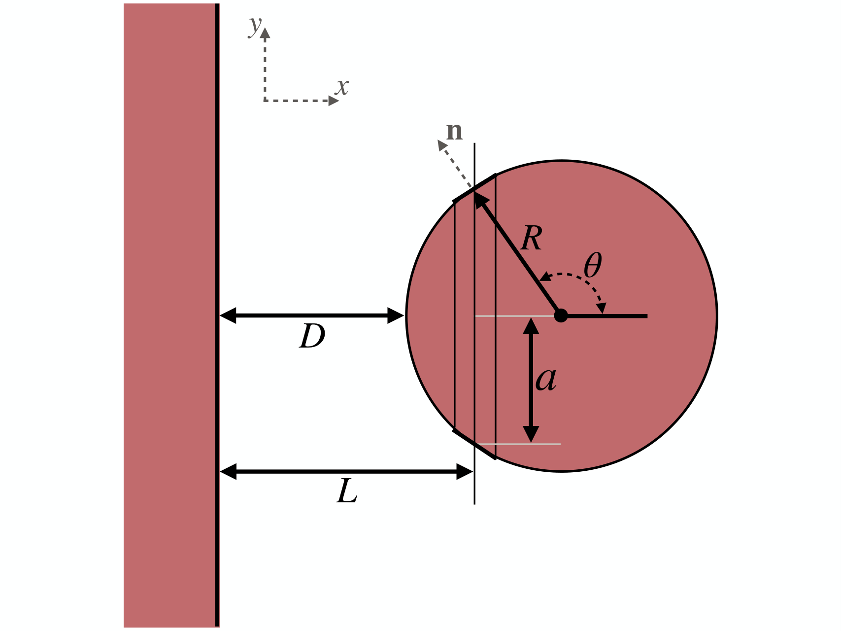
As a specific example, let us consider a prototypical Casimir experiment with two infinitely-dense, parallel plates, separated by a vacuum gap. The left panel of Fig. 4 depicts the configuration and the surface of a rectangular box. Our primary interest in this example is the calculation of the Symmetron pressure on one of the plates, and we can make use of the analytical field profile derived using Eq. (34).

Given the specific choice of the enclosing surface, the matter of the plate does not contribute to the integral in Eq. (56). For the Symmetron field, we have
| (57) |
From the symmetry of the problem, the only component of the force is in -direction, and it reads as
| (58) |
where “in” and “out” denote the solutions inside and outside of the gap. The latter can be obtained by using the general form for the solution inside and assuming an infinitely wide gap. Primes denote derivatives with respect to the -coordinate.
The fifth force per area on the plate the follows:
| (59) |
where a useful identity for Jacoby elliptic functions has been employed
| (60) |
An alternative approach for calculating the pressure would have been to calculate the energy density stored in the scalar field configuration, and take the derivative with respect to the plate separation . Direct computation shows agreement with the result presented in Eq. (59).
4 Laboratory tests
Laboratory experiments that are sensitive to the effects of weak forces are capable of providing useful constraints on the screening mechanisms. We will schematically divide such experiments into two broad categories. The experiments in the first category constrain the screening mechanisms due to the fifth force effects on test objects, such as atoms or neutrons. Such experiments are referred to as “indirect measurements” below, and include atomic interferometry Burrage et al. 2015; Burrage and Copeland 2016; Hamilton et al. 2015; Burrage et al. 2016; Jaffe et al. 2017; Sabulsky et al. 2019, atomic spectroscopy Brax and Burrage 2011; Brax et al. 2023 and bouncing neutron Cronenberg et al. 2018 experiments. On the other hand, the experiments that try to directly measure the fifth forces between extended objects are referred to as “direct force measurements”, which include Casimir Decca et al. 2005; Decca et al. 2003; Almasi et al. 2015; Sedmik and Brax 2018; Brax et al. 2010 and torsion balance experiments Adelberger 2002.
We make this distinction primarily because of the unique technical challenges associated with making robust and reliable theoretical predictions for those two classes of experiments. While in the first class of experiments, the analytical approximations have proven to be very useful and accurate enough, the direct force measurements often involve very complex density geometries, and their analysis requires more careful numerical modeling. Despite differences in modeling, it is important to combine the constraints derived in different experiments since they often cover complementary regions of the parameter space. Fig. 5 represents a summary of constraints on symmetron models from laboratory experiments. A similar summary for chameleon models can be found in Ref. Brax et al. 2022.
4.1 Direct force measurements
Casimir Experiments: The primary purpose of Casimir-force experiments is the measurement of the force due to modified vacuum energy density in presence of conducting extended bodies (see Sparnaay 1958; van Blokland and Overbeek 1978; Lamoreaux 1997 for historical realizations of the experiment, and Decca et al. 2005; Decca et al. 2003 for modern and more precise experiments). Such experiments, however, can also be used for constraining additional (classical) forces Decca et al. 2005; Decca et al. 2003. It is therefore natural to consider the chameleon and symmetron fifth forces in the context of such experiments. Modern Casimir experiments probe distance scales of m and are therefore sensitive to large effective scalar-field masses.
The main theoretical complication lies in the difficulty of obtaining accurate estimates of scalar field profiles and fifth forces in complex configurations of realistic experiments. While the earlier Casimir force measurements were performed using two parallel plates, see e.g. Ref Almasi et al. 2015, many modern setups can be approximated as a sphere placed in front of the source plate Mohideen and Roy 1998; Harris et al. 2000; Lamoreaux 1997; Decca et al. 2005; Chen et al. 2016 (see, however, Bressi et al. 2002; Zou et al. 2013 for modern experimental configurations with planar geometry). The schematic setup of interest is depicted in the right panel of Fig. 4.
A careful treatment of systematic effects is essential to produce reliable constraints on fifth-force models. For example, lateral forces and roughness are not captured by the proximity force calculation (Neto et al. 2005; Rodrigues et al. 2006) and the surfaces used have a finite conductivity (Lambrecht and Reynaud 2000), both of which must be accounted for. Since the focus of this review is on the reconstruction of the scalar fifth force profiles, we do not discuss these effects further here, but see e.g. Reynaud and Lambrecht 2017 for a review.
Analytical progress can be made in the limiting cases of very small and large spheres. The exposition below focuses on symmetrons, and largely follows Elder et al. 2020. In the significantly simpler small-sphere limit, , we can treat the sphere as a test mass that does not significantly alter the ambient field profile sourced by the plate. The force on the sphere with mass , in this case, can then be computed as
| (61) |
where is the screening factor introduced in Subsection 2.1, and is the analytically solvable field profile of the isolated plate (see the end of Subsection 3.1). As a result we can obtain an accurate analytical force estimate when .
The situation is more subtle in the opposite limit of a very large sphere, . In this limit, the configuration can be approximated by a collection of parallel plates of varying gap openings by dividing the sphere into co-centric rings facing the plate. The exact (although not explicit) parallel-plate solutions can then be used to obtain the total force on the sphere. This approach is essentially the extension of the proximity force approximation widely employed for calculating the quantum Casimir forces (see e.g. Dalvit and Onofrio 2009; Krause et al. 2007), and it has been used for studying Chameleon models in Casimir experiments Brax et al. 2007.
Given the exact parallel-plate pressures for each of the co-centric rings, the total force can be expressed as
| (62) |
where is the -distance between the plate and a ring (see Fig.4 for the notation).
We expect both the approximate approaches to fail in the intermediate regime in between of and . For such intermediate radii we should rely on exact numerical integration of the field profiles, which can be performed using any of the methods explained in Section 3 with sufficient care toward choosing an appropriately large box size so that the boundary effects do not alter the physical conclusions. Ref. Elder et al. 2020 presents a detailed analysis of the plate-sphere configuration in symmetron models and finds that the proximity approximation provides an acceptable accuracy for large-enough spheres. The analysis also validates the results of the large and small sphere approximations. A similar analysis has been performed for chameleon models Brax et al. 2007; Brax et al. 2022. Interestingly, it has been demonstrated that, unlike the case of symmetrons, the proximity force approximation in the case of chameleons does not reproduce the numerical results even in the limit of large spheres. For chameleons, the approach based on the screening factor calculation for the sphere leads to more reliable analytical estimates Brax et al. 2022. This stresses once more the strong model-dependence of screening mechanisms.
Torsion Balance: One version of torsion-balance experiments Adelberger 2002 consists of two parallel cylinders. The bottom disc is turned uniformly while the upper one is a torsion pendulum and can rotate freely. The discs have regularly spaced holes with missing mass. In presence of a fifth force the torsion pendulum would experience a torque when its holes move across the holes of the lower rotating disc. The scalar field configuration is challenging to obtain in such a complex geometry. Particularly, the parallel-plane results can be used to obtain qualitatively robust results Brax and Davis 2015. However, edge effects require a refined analytical modeling and numerical treatment.
Initial results have been obtained by numerically solving the field profile using the conjugate gradient minimization of the Hamiltonian of the system Upadhye et al. 2006. This direct numerical approach, however, can become prohibitive in certain parts of parameter space which require very fine grid sizes compared to the geometry of the problem. Refs. Upadhye 2012; Upadhye 2013 offered an approximate treatment of the system by introducing the so-called 1-dimensional plane-parallel approximation. The essential idea is to approximate the field on the pendulum cylinder surface by the corresponding surface field in a parallel-plate setup with the gap size corresponding to the distance of the point of interest and the nearest point on the bottom cylinder. Such an approach is similar to the proximity force approximation discussed earlier, and gives qualitatively correct results on the torque, although it quantitatively underestimates the numerical results.
4.2 Indirect measurements
Atomic Interferometry: Atomic interferometry is a sensitive probe of gravitational free-fall acceleration. Such experiments are realized inside a vacuum chamber with a spherical source near its center. Atomic matter waves are beam-split and travel in free fall until their interference. The primary observable of interest is the accumulated phase difference between the split matter waves, which is linearly proportional to the acceleration of atomic clouds.
In the context of screening mechanisms, the acceleration is due to both gravity and the fifth force. The entire experiment is carried out inside a vacuum chamber with thick and dense walls. As a result the field profile inside the chamber is independent of the ambient field profile outside. In order to induce fifth forces, a macroscopic source with e.g. spherical shape is placed near the center of the chamber. The total acceleration can be determined using the screening factors and of the atom and the source, and for Chameleon theories can be written as
| (63) |
This expression includes both the gravitational acceleration and the acceleration due to fifth forces. A central feature of such configurations is that, while the source could be screened and have , the atoms are typically not, , and the overall fifth-force acceleration is not doubly-suppressed.
Atomic interferometry experiments in the context of screened fifth force searches have been carried out by two independent groups Hamilton et al. 2015; Jaffe et al. 2017; Sabulsky et al. 2019. Analytical modeling approximations have been extensively validated using exact numerical integration of the scalar field equations in the context of such experiments Elder et al. 2016.
Bouncing Neutrons and other methods: Experiments including neutrons have been designed in order to measure the energy levels of quantum-mechanical particles in the gravitational field. In presence of an additional fifth force, the energy levels are perturbed and the parameters of the screening mechanisms can be strongly constrained. Such bouncing neutron experiments have been analyzed in the context of symmetrons in Cronenberg et al. 2018.
A logically similar method is to compute the shifts in atomic energy levels due to the fifth force on electrons Brax and Burrage 2011; Brax et al. 2023. The effect can be analytically described using the screening factor of the nucleus. In both the bouncing neutron and atomic spectroscopy methods the effect of the fifth force constitutes in perturbing the Hamiltonian of either the neutrons or electrons. Once the perturbed Hamiltonian is computed, the shifts in energy levels can be estimated by perturbation theory.
5 Astrophysical scales
5.1 Stars
5.1.1 Hydrostatic equilibrium - stellar structure and evolution
In the presence of a fifth force, the structure and evolution of stars will be altered compared to GR, allowing stellar objects to be utilised as probes of such modifications. The gravitational collapse of a star is halted by its internal pressure such that, if gravity is stronger, then the required outward pressure must also increase, so stars are forced to burn their fuel at a faster rate. This shortens the lifetime of the star and will make them appear brighter. The opposite would occur if the modification to gravity weakened the attractive force within the star.
To quantitatively study the impact of modifications to gravity, the only equation one needs to alter is the criterion for hydrostatic equilibrium (Koyama and Sakstein 2015; Saito et al. 2015)
| (64) |
for pressure , density and where is the mass enclosed at radius . In standard gravity , and is more generally given in terms of the , and parameters (Gleyzes et al. 2015) as
| (65) |
The mere existence of stars already requires , since below this value gravity becomes repulsive near the center of the star (Saito et al. 2015).
In the simplest models, one supposes that a star has a polytropic equation of state, , for positive constants and . One can then define dimensionless variables in terms of the central density and pressure to be
| (66) |
and thus arrive at the modified Lane-Emden equation (Koyama and Sakstein 2015)
| (67) |
which has boundary conditions , .
To make progress, one now needs to couple this equation with other equations describing stellar evolution. By using analytic approximations for the temperature profile and assuming a polytropic index , Koyama and Sakstein 2015 demonstrated that increasing resulted in a reduction of the stellar luminosity at fixed mass, with stronger modifications for low mass stars since these are supported by gas pressure, rather than radiation pressure. This constrains to be . Similarly, Sakstein 2015a; Sakstein 2015b showed that the weakening of gravity within astrophysical bodies in scalar-tensor theories will increase the minimum mass a star must have to sustain hydrogen burning which, given the observed masses of Red Dwarf stars (which are greater than (Ségransan et al. 2000)), lead to similar constraints, ruling out . Modifications of gravity can also change the radius of brown dwarfs from their GR prediction () to arbitrarily large values if gravity is weaker, or down to if it is stronger.
To go beyond these semi-analytic models, one must solve all the relevant stellar structure equations simultaneously. This is commonly achieved by modifying the gravity model in the publicly available Modules for Experiments in Stellar Astrophysics (MESA) code (Paxton et al. 2011; Paxton et al. 2013; Paxton et al. 2015; Paxton et al. 2018; Paxton et al. 2019; Jermyn et al. 2022).
After making such modifications, one can investigate the effect on different aspects of stellar evolution. For example, by considering the RGB phase, Chang and Hui 2011 saw that, in Chameleon models, red giants can be significantly smaller (by tens of percent) and hotter (by hundred of Kelvins) than their GR counterparts. This effect is particularly pronounced in red giants since main sequence stars are much denser and thus have a suppressed scalar charge, whereas the outer envelope of red giants remains unscreened. If one considers galileons (Gleyzes et al. 2015) exhibiting Vainstein screening, one finds that it is the main-sequence stars which are most strongly affected (Koyama and Sakstein 2015), and have a smaller effective temperature than GR stars at the same point in the Hertzsprung–Russell diagram. While such an effect could be degenerate with metallicity, modified gravity theories leave distinct evolutionary tracks in the Hertzsprung–Russell diagram, allowing these objects to constrain such models. In the context of general modified gravity theories Saltas and Lopes 2019 and Saltas and Christensen-Dalsgaard 2022 have investigated the changes in the solar sound speed using analytical approximations and MESA simulations. These studies have concluded that precise helioseismic observations are able to improve the constraints on the fifth force coupling strength , and have derived an approximate constraint of at the confidence level.
5.1.2 Out of equilibrium - stellar oscillations
Until now we have only considered stars in equilibrium. Moving beyond this, suppose one can consider small radius perturbations in the star which obey the equation
| (68) |
In the absence of modified gravity, the period of small oscillations is found to be
| (69) |
Hence any enhancement in the strength of gravity ( with ) would reduce the period (Jain et al. 2013). The change in the period can be as large as 30% for couplings in chameleon screened theories (Sakstein 2013). This would be important for Cepheids – massive stars which pulsate with periods ranging from days to weeks when they pass through the instability strip – since the relation between their luminosity and period is used to determine their distance. This allows one to measure the strength of gravity in e.g. the Large Magellanic Cloud (Desmond et al. 2021) by modeling the internal properties of Cepheids with MESA.
Moreover, since Cepheids are used in the construction of the distance ladder for local measurements of , an incorrect distance estimation can bias the inferred value of . Indeed, Desmond et al. 2019 found that a fifth force with 5-30% the strength of gravity can reduce the Hubble tension. A similar effect can be obtained by instead calibrating to the TRGB (Desmond and Sakstein 2020); if the hydrogen burning shell become unscreened, then the luminosity at the TRGB would be reduced (Sakstein et al. 2019) and thus distances based on this feature would be overestimated. Fifth-forces can therefore reduce the locally inferred value of thus reducing or alleviating the Hubble tension. Högås and Mörtsell 2023 have studied the period-luminosity relation in the context of the symmetron theory. While this theory has been shown to worsen the Hubble tension, the distance ladder measurements impose strong constrains on the symmetron Compton wavelength.
Using the same notation as above, for Vainshtein screened theories, one can write and linearise the pressure and potential to obtain a modified Linear Adiabatic Wave Equation (Sakstein et al. 2017)
| (70) |
where
| (71) |
and a subscript ‘0’ denotes an unperturbed quantity (see Sakstein 2013 for the chameleon-screened version of this equation). For stars in GR, this results in unstable stars if , whereas in beyond Horndeski theory there is a second instability for sufficiently large , since this will result in (Sakstein et al. 2017). Using MESA, Sakstein et al. 2017 showed that the modification to the period-luminosity relation for Cepheids also holds for these theories, and thus the distances inferred using this method can be compared to that from the TRGB to constrain .
5.2 Screening maps
When determining whether a given object is screened or unscreened, one often computes properties of the local gravitational field: the potential, , for chameleons, the acceleration, , for kinetically screened theories, or the local curvature (e.g. the Kretschmann scalar, ) in the presence of Vainshtein screening. These all have contributions from the object itself, but also from an object’s local environment. Particularly for astrophysical tests, it is therefore imperative to produce maps of these quantities to identify the screened and unscreened regions of the local Universe.
The Poisson equation for the potential, , in the presence of a density perturbation, , is modified in gravity to be
| (72) |
where is perturbation to Ricci scalar and is the scale factor. By integrating to obtain a dynamical mass, , and comparing to true “lensing” mass, , one can calculate a proxy for the degree of screening, (Zhao et al. 2011; Schmidt 2010). In this case, , where corresponds to a perfectly screened object, and is completely unscreened. Although this offers a useful metric for quantifying the degree of screening, we often do not have access to both the lensing and dynamical masses of objects, so must rely on alternative methods.
Cabré et al. 2012 were the first to produce maps of the local gravitational potential for use in quantifying the degree of screening. For a set of galaxies of mass and virial radii , they compute the external contribution to to be
| (73) |
where is the Compton wavelength of the field, and is the distance to the th galaxy. One must introduce a cut-off based on the Compton wavelength, otherwise the above sum would diverge. This screening map covered and the Sloan Digital Sky Survey (SDSS) footprint, since it was produced predominantly from a compilation of the SDSS group catalog (Yang et al. 2007), alongside other catalogs (Abell et al. 1989; Ebeling et al. 1996; Karachentsev et al. 2004; Lavaux and Hudson 2011). The approximations used were tested and calibrated against -body simulations (Zhao et al. 2011).
A more sophisticated analysis was performed by Desmond et al. 2018, who extended these methods to produce full-sky maps up to , as well as maps of and . Galaxies from the 2M++ galaxy catalog (Lavaux and Hudson 2011) were matched to rockstar (Behroozi et al. 2013) halos from the DARKSKY-400 simulation (Skillman et al. 2014) using the abundance matching method of Lehmann et al. 2017. Assuming these halos have Navarro–Frenk–White (NFW) density profiles (Navarro et al. 1997), and were computed using all objects within of a given point using standard formulae (Cole and Lacey 1996). To compute the curvature, was approximated to be the sum of point mass contributions; this neglects the extended nature of halos and the non-linearity of this quantity, so should be treated as an order of magnitude approximation. To account for galaxies in halos which are too faint to be observed, correction factors for each quantity were applied by comparing to results from -body simulations. To account for mass which does not reside in halos, a single constrained density field inferred using the Bayesian Origin Reconstruction from Galaxies (borg) algorithm (Jasche and Wandelt 2012; Jasche and Wandelt 2013; Jasche et al. 2010; Jasche et al. 2015; Lavaux and Jasche 2016) applied to the 2M++ galaxy catalog was used.
Instead of computing screening proxies, one could directly compute the profiles of the dynamical fields which result in a modification to gravity, although one must do this separately for each theory one wishes to test. As part of the LOCal Universe Screening Test Suite (locusts) project, Shao et al. 2019 solved for the scalar field for Hu-Sawicki gravity applying the ecosmog (Li et al. 2012; Li et al. 2013a; Li et al. 2013b) code to a constrained -body simulation from the elucid project (Wang et al. 2014; Wang et al. 2016) (inferred using the SDSS DR7 galaxy catalog), using 20 values in the range .
Both the borg and elucid density fields used to produce screening maps are constrained assuming no modification to gravity. Hence, these maps implicitly assume that the low redshift Universe has matter fields which are similar for all reasonable modified gravity and CDM models on the scales of the reconstruction. The first constrained density fields which include the effects of modified gravity have now been produced (Naidoo et al. 2022) from CosmicFlows peculiar velocity data (Kourkchi et al. 2020), through an extension of the ICeCoRe package (Doumler et al. 2013). By applying a Wiener filter (Zaroubi et al. 1995) to obtain the linear density and velocity fields, applying the reverse Zeldovich approximation (Doumler et al. 2013), then adding fluctuations in poorly constrained regions, they obtain estimates for the initial conditions at . They then run simulations using the mg-picola (Winther et al. 2017) implementation of the COmoving Lagrangian Acceleration (COLA) method (Tassev et al. 2013) for nDGP and models, which solves for particle trajectories in the frame of the reference given by Lagrangian perturbation theory. The current implementation neglects the scale-dependence of the growth function in when generating constrained realisations, hence they find that it is better to generate constrained simulations from CDM initial conditions than the ones they infer. Future work should be dedicated to producing fully-consistent constrained simulations and moving away from the linear approximation required in this reconstruction Naidoo et al. 2022. Phenomenological approaches to incorporating screening effects in quasi-linear regimes of structure formation could offer additional insights in understanding the large-scale environmental effects on screening dynamics Fasiello and Vlah 2017.
5.3 Galaxy morphology
5.3.1 Thin-shell screened theories
In thin-shell screened theories where the degree of screening is determined by the Newtonian potential, one can define a cut-off, , such that objects with potentials below this value are unscreened and experience a fifth-force, and all other objects are screened. If , then main sequence stars will always be screened, since this is the potential at their surfaces, irrespective of their environment. However, if the local gravitational potential is below this value, the surrounding gas and dark matter will be unscreened, and hence feel an additional force. If there exists a gradient in the field responsible for the fifth force, then the gas and dark matter will be accelerated whereas the stars will not, leading to an offset between the centre of mass of the stars and the remaining mass of the galaxy. This offset will be stabilised by the induced gravitational potential, and this will also induce a warp in the stellar disk. Thus, two morphological signatures are to be expected in such a theory: (1) an offset parallel to the local gravitational field between the stars and gas of galaxies in regions of low gravitational potential and (2) a warping of the stellar disk into a characteristic ‘U’ shape (Jain and VanderPlas 2011).
Initial studies (Vikram et al. 2013) of these phenomena utilising the screening maps of Cabré et al. 2012 (see Subsection 5.2) and, combining data from the ALFALFA Giovanelli et al. 2005 and SDSS Abazajian et al. 2009 surveys, found no evidence for screened fifth forces, but the constraints were not competitive with other astrophysical probes. More recently, galactic morphology has played an increasingly important role in constraining such theories (Desmond et al. 2018a; Desmond et al. 2018b; Desmond et al. 2019), with the screening maps of Desmond et al. 2018 being used to determine which objects are unscreened and to predict the magnitude and direction of the offsets and warps. The most recent constraints find that a fifth force with must have a strength at least as small as 0.8 at confidence (Desmond and Ferreira 2020). Hu-Sawicki with is ruled out, resulting in practically all astrophysical objects being screened in the surviving region of parameter space, and hence all astrophysically relevant models are disfavoured. The modeling of other astrophysical effects for these constraints has been shown to be robust when calibrated against hydrodynamical CDM simulations (Bartlett et al. 2021).
5.3.2 Vainshtein screened theories
One of the main astrophysical tests of the Vainshtein mechanism relies on the difference in coupling for non-relativistic matter () and black holes () and was proposed by Hui and Nicolis 2012. This extreme difference means that, if the non-relativistic matter in a galaxy (stars, gas, dark matter) is falling down a gradient in the galileon field, then the supermassive black hole at its centre lags behind as it does not experience the fifth force. This offset is stabilised by the induced gravitational potential, and thus one would expect to see an offset between the black hole near a galaxy’s centre and its centroid, as measured by the stars.
This test was first performed by Sakstein et al. 2017 by considering the black hole–galaxy offset in M87, utilising the analysis of Asvathaman et al. 2017. Here the galileon profile was determined analytically assuming spherical symmetry (Eq. (22)), which was shown to be an excellent approximation for cosmological simulations (see e.g. Ref. Schmidt 2009). As shown in Fig. (6), was found to be excluded for cross-over scales .
Bartlett et al. 2021a extended these results by comparing the galaxy centroids to the X-ray and radio positions of active galactic nuclei (AGN) in a sample of 1916 galaxies compiled in (Bartlett et al. 2021b). They considered the galileon field sourced by large scale structure, utilising a suite of constrained -body simulations to produce maps of dark matter in the nearby Universe to predict both the magnitude and direction of the offset. By comparing to observations, the constraints on were found to be tighter than those obtained from M87, with ruled out at confidence (see Fig. (6)), although these constraints are applicable to larger . We note that the constrained simulations were constructed assuming CDM, and thus these constraints are only applicable for models which give rise to similar large scale structure as CDM, and only affect objects on smaller scales. Furthermore, the Vainshtein mechanism was approximated as a hard cut-off, such that on large scales the galileon field traces the gravitational potential, but above some wavenumber the galileon field is set to zero. This is likely to be a less accurate approximation than that used by Sakstein et al. 2017, although the advantage of using a statistical sample is that the non-galileon effects which were ignored in Sakstein et al. 2017 were empirically modelled and marginalized over.
5.4 Halo properties
In GR, gravity determines the formation and growth of dark matter halos. Their abundance and internal structure can be modified in presence of fifth forces, which might be partially unscreened especially for objects with smaller masses and on the outskirts of halos. Since halos are strongly non-linear structures, N-body simulations have been the primary framework for deriving a quantitative understanding of these effects.
Modeling halo structure in modified gravity theories has been the focus of extensive past work, such as Refs. Schmidt et al. 2009; Li and Hu 2011; Pourhasan et al. 2011; Lombriser et al. 2012; Lombriser et al. 2013; Lombriser et al. 2014; Shi et al. 2015; Mitchell et al. 2019 for chameleon theories, Refs. Schmidt et al. 2010; Barreira et al. 2014; Falck et al. 2014; Mitchell et al. 2021; Pizzuti et al. 2022 for Vainshtein mechanism, and Ref. Clampitt et al. 2012 for symmetrons. Additionally, environmental dependences for both chameleon and Vainshtein mechanisms have been studied in Refs. Schmidt 2010; Falck et al. 2015.
Screening efficiency depends on the halo mass, and in the case of chameleon theories less massive halos tend to be unscreened. For Vainshtein, on the other hand, screening is less sensitive to the mass, and practically all halos are screened Schmidt 2010; Falck et al. 2015. As explained in Subsection 2.2, even though the inner regions of NFW halos in Vainstein-screened theories are expected to be fully screened, one expects non-vanishing fifth force outside the virial radius. Simulations agree well with this theoretical prediction, with certain variation near the outskirts of the halos which is likely due to the breakdown of the NFW approximation (Schmidt 2009; Khoury and Wyman 2009; Schmidt et al. 2010).
As far as population-level mass distribution is concerned, it has been established that partially screened fifth forces induce significant modifications in the differential halo mass function , see e.g. Schmidt et al. 2009; Lombriser et al. 2013; Shi et al. 2015. While the exact results depend strongly on the model parameters, a general trend is that the distribution of very heavy halos is not affected. The main difference can be seen below a certain mass threshold, where halos are more abundant than in General Relativity. At even lower masses, halos are more abundant in GR, because such smaller halos are more efficiently absorbed by larger ones.
In CDM, halos have universal density profiles described by the NFW parametrization:
| (74) |
where is a characteristic density, and is a characteristic scale for a halo. The compactness (concentration) of the profile is determined as the ratio of the virial radius and ; . The concentration and the characteristic density are connected via
| (75) |
where is the critical density of the Universe, and .
Earlier studies, such as Refs. Shi et al. 2015; Lombriser et al. 2014 have examined the halo profiles in N-body simulations and found that NFW is still an appropriate description, especially for larger halos. The profiles however can be more compact compared to GR. Detailed investigation of such an effect can be found in e.g. Refs. Shi et al. 2015; Mitchell et al. 2019 which found that halos with masses below a certain threshold are typically more concentrated. This, however, also depends on redshift, with the effect diminishing at relatively higher redshifts.
5.5 Splashback
In addition to modifying the halo concentrations and their mass function, fifth forces can also imprint non-trivial and potentially observable effects on the halo profiles. For larger, cluster-size halos this primarily concerns the outskirts of the density profiles, where fifth forces might be unscreened, hence significantly altering the dynamics of collapsing matter shells. In recent years, the splashback feature has gained importance as a physically motivated boundary of halos. This feature corresponds to the dividing boundary of single-streaming and multi-streaming regions and manifests itself as a steepening at outer regions Diemer and Kravtsov 2014. The splashback location can in principle be inferred by measuring the radial distribution of subhalos, and assuming matter follows the same distribution More et al. 2016; Baxter et al. 2017; Chang et al. 2018; Shin et al. 2018. Additionally, dedicated lensing measurements can also be used Umetsu and Diemer 2017; Contigiani et al. 2018.
The position of the splashback feature is sensitive to any additional interactions and has been investigated in the context of gravity and nDGP by Adhikari et al. 2018. Here the authors have used both semi-analytical and N-body approaches to predict the changes in splashback location. For symmetrons, splashback has been investigated in Contigiani et al. 2019 by extending the self-similar collapse approach Fillmore and Goldreich 1984; Bertschinger 1985. The latter approach, while not quantitatively very accurate, allows gaining important insights into halo growth in presence of fifth forces. We will use this approach to demonstrate the changes in splashback location.
We will focus on the collapse in Einstein de-Sitter (EdS) universe, and enforce the mass profile to satisfy a self-similar form:
| (76) |
where is the turn-around radius at time , and is the mass within the radius . The mass withing turn-around radius grows with scale factor as , with accretion rate , and in EdS is a power-law in cosmic time .
In absence of fifth force the shell variables can be rescaled such that all the shells satisfy the same equation of motion
| (77) | ||||
| (78) |
where we have labeled each shell by its turn-around time and radius , and have introduced , and . This system, complemented by initial conditions are , , can be iteratively solved until a converged mass-profile is obtained. The time-dependence of the density profile is determined in terms of the critical density and . These equations can also be formulated for other -dimensional configurations Fillmore and Goldreich 1984, as well as tri-axial collapse Lithwick and Dalal 2011. The framework can also be extended to full CDM backgrounds Shi 2016.

Once the self-similar halo profile is obtained as function of redshift, the symmetron field profiles can be computed with one of the methods introduced in Section 3. The extra force on outer shells can be added in Eq. (77) in order to study the dynamics of the outer-most collapsing shells. It should be noted that in the cosmological context presented here, the symmetron is fully screened at higher redshift. The unscreening redshift, , is determined by the condition . Fig. 7 demonstrates the fifth-force profiles as a function of redshift, and the resulting effect on splashback location. From the right panel of the same figure it is clear that the innermost regions of the overdensity always stay screened. Substantial fifth forces start appearing in the outer regions when the condition is satisfied. At some point, a thin shell forms and the force gets concentrated in a narrow radial region. Due to this behaviour there exists an optimal value of which maximizes the change in splashback location due to fifth forces.
6 Conclusions
The discovery of late-Universe cosmic acceleration motivated the extensive studies of alternatives to Einstein’s theory of General Relativity. Such modified gravity theories generically involve additional scalar degrees of freedom. When such fields couple non-trivially to gravity and matter fields, they exert additional, “fifth” forces on matter particles. The presence of fifth forces leads to remarkable variety of phenomenological effects, ranging from cosmologically large scales down to microscopic effects.
At large and linear scales the novel effects have been relatively well-understood in terms of modified growth of structure, which in modified gravity can be scale- and time-dependent, and modified gravitational lensing. Significant progress has been made, first of all, by employing perturbation theory techniques in order to derive generic and largely model-independent observables, see e.g. Pogosian and Silvestri 2016; Amendola et al. 2018. Moreover, Effective Field Theory approaches have been very successful for systematically deriving unified prescriptions of linear perturbations Gubitosi et al. 2013; Gleyzes et al. 2013; Creminelli et al. 2014; Bellini and Sawicki 2014. Such unified approaches have been efficiently implemented in Einstein-Boltzmann numerical solvers Hu et al. 2014; Raveri et al. 2014; Zumalacárregui et al. 2017; Bellini et al. 2020.
On smaller scales the dynamics of scalar fields exhibit highly non-linear behaviour, and lead to remarkable density-dependent screening effects. In this short review we have summarized the main classes of screening mechanisms and have provided a broad summary of numerical and analytical methods developed in the context of non-linear dynamics. Unlike the linear regime, in screening regimes scalar fields behave in a very model-dependent way. Even though at the theoretical level screening mechanisms can be categorized into distinct classes, such as chameleons, symmetrons, and Vainshtein mechanisms, their precise phenomenological descriptions are given at a model-by-model basis. Even very similar mechanisms, such as chameleons and symmetrons can often require different analysis approaches. An interesting and non-trivial example of this is the study of Casimir fifth forces in sphere-plane configurations, which closely resemble modern experimental setups. For example, the proximity-force approximation, explained in Subsection 4.1 can provide accurate description for the system for symmetrons, while fail for chameleons.
Numerical approaches are typically required in order to asses the validity of analytical approximations for a specific model. Providing an introductory summary of numerical algorithms is among the central topics of this review. While current numerical solvers have been designed with specific models in mind, most of the numerical approaches are applicable for a broad range of theories. This motivates for developing unified solver packages. The Finite-Elements-Based solvers introduced in Subsection 3.2, particularly, posses very favourable dimensional scaling properties. A unified FEM-based code can be applied not only to complex laboratory configurations, but also to astrophysical and cosmological scenarios.
Identifying novel regimes where modified gravity can be tested is another promising avenue. Particularly, as outlined in Subsection 5.2, screening maps of the large-scale structure are useful for systematically exploring regions with discovery potential. To this end, constrained simulations are important, in order to correctly account for environmental effects. In some of the existing studies GR-based constrained simulations have been employed. Self-consistent modified gravity constrained simulations, such as the one presented in Naidoo et al. 2022, will play an important role in producing precise screening maps.
Testing modified gravity theories in non-linear regimes will provide invaluable insights about the nature of gravitational interactions. At the same time, robust modeling of non-linear phenomena is often very challenging and extensive cross-domain effort is required. As the precision of both the laboratory and astrophysical tests is drastically improving, approximate methods need to be replaced with more accurate approaches.
Funding
V.V. is supported by the WPI Research Center Initiative, MEXT, Japan and partly by JSPS KAKENHI grant 20K22348. D.J.B. acknowledges support by the Simons Collaboration on “Learning the Universe”.
Data Availability Statement
Figures 1, 2 and 3 are adapted from Vardanyan 2019, Figures 4 and 5 are adapted from Elder, Vardanyan, et al. Elder et al. 2020 , Figure 6 is adapted from Bartlett et al. 2021a. Figure 7 is adapted from Contigiani et al. 2019.
Conflicts of Interest
The authors declare no conflict of interest.
References
- Perlmutter et al. (1999) Perlmutter, S.; et al. Measurements of and from 42 high redshift supernovae. Astrophys. J. 1999, 517, 565–586, [astro-ph/9812133]. https://doi.org/10.1086/307221.
- Riess et al. (1998) Riess, A.G.; et al. Observational evidence from supernovae for an accelerating universe and a cosmological constant. Astron. J. 1998, 116, 1009–1038, [astro-ph/9805201]. https://doi.org/10.1086/300499.
- Copeland et al. (2006) Copeland, E.J.; Sami, M.; Tsujikawa, S. Dynamics of dark energy. Int. J. Mod. Phys. D 2006, 15, 1753–1936, [hep-th/0603057]. https://doi.org/10.1142/S021827180600942X.
- Silvestri and Trodden (2009) Silvestri, A.; Trodden, M. Approaches to Understanding Cosmic Acceleration. Rept. Prog. Phys. 2009, 72, 096901, [arXiv:astro-ph.CO/0904.0024]. https://doi.org/10.1088/0034-4885/72/9/096901.
- Clifton et al. (2012) Clifton, T.; Ferreira, P.G.; Padilla, A.; Skordis, C. Modified Gravity and Cosmology. Phys. Rept. 2012, 513, 1–189, [arXiv:astro-ph.CO/1106.2476]. https://doi.org/10.1016/j.physrep.2012.01.001.
- Joyce et al. (2015) Joyce, A.; Jain, B.; Khoury, J.; Trodden, M. Beyond the Cosmological Standard Model. Phys. Rept. 2015, 568, 1–98, [arXiv:astro-ph.CO/1407.0059]. https://doi.org/10.1016/j.physrep.2014.12.002.
- Koyama (2016) Koyama, K. Cosmological Tests of Modified Gravity. Rept. Prog. Phys. 2016, 79, 046902, [arXiv:astro-ph.CO/1504.04623]. https://doi.org/10.1088/0034-4885/79/4/046902.
- Ade et al. (2016) Ade, P.A.R.; et al. Planck 2015 results. XIV. Dark energy and modified gravity. Astron. Astrophys. 2016, 594, A14, [arXiv:astro-ph.CO/1502.01590]. https://doi.org/10.1051/0004-6361/201525814.
- Pogosian and Silvestri (2016) Pogosian, L.; Silvestri, A. What can cosmology tell us about gravity? Constraining Horndeski gravity with and . Phys. Rev. 2016, D94, 104014, [arXiv:astro-ph.CO/1606.05339]. https://doi.org/10.1103/PhysRevD.94.104014.
- Will (1993) Will, C.M. Theory and experiment in gravitational physics; 1993.
- Khoury and Weltman (2004a) Khoury, J.; Weltman, A. Chameleon cosmology. Phys. Rev. D 2004, 69, 044026, [astro-ph/0309411]. https://doi.org/10.1103/PhysRevD.69.044026.
- Khoury and Weltman (2004b) Khoury, J.; Weltman, A. Chameleon fields: Awaiting surprises for tests of gravity in space. Phys. Rev. Lett. 2004, 93, 171104, [astro-ph/0309300]. https://doi.org/10.1103/PhysRevLett.93.171104.
- Brax et al. (2004) Brax, P.; van de Bruck, C.; Davis, A.C.; Khoury, J.; Weltman, A. Detecting dark energy in orbit: The cosmological chameleon. Phys. Rev. D 2004, 70, 123518, [astro-ph/0408415]. https://doi.org/10.1103/PhysRevD.70.123518.
- Hinterbichler and Khoury (2010) Hinterbichler, K.; Khoury, J. Symmetron Fields: Screening Long-Range Forces Through Local Symmetry Restoration. Phys. Rev. Lett. 2010, 104, 231301, [arXiv:hep-th/1001.4525]. https://doi.org/10.1103/PhysRevLett.104.231301.
- Hinterbichler et al. (2011) Hinterbichler, K.; Khoury, J.; Levy, A.; Matas, A. Symmetron Cosmology. Phys. Rev. D 2011, 84, 103521, [arXiv:astro-ph.CO/1107.2112]. https://doi.org/10.1103/PhysRevD.84.103521.
- Vainshtein (1972) Vainshtein, A.I. To the problem of nonvanishing gravitation mass. Physics Letters B 1972, 39, 393–394. https://doi.org/10.1016/0370-2693(72)90147-5.
- Nicolis et al. (2009) Nicolis, A.; Rattazzi, R.; Trincherini, E. Galileon as a local modification of gravity. Phys. Rev. D 2009, 79, 064036. https://doi.org/10.1103/PhysRevD.79.064036.
- Babichev and Deffayet (2013) Babichev, E.; Deffayet, C. An introduction to the Vainshtein mechanism. Class. Quant. Grav. 2013, 30, 184001, [arXiv:gr-qc/1304.7240]. https://doi.org/10.1088/0264-9381/30/18/184001.
- Burrage and Sakstein (2016) Burrage, C.; Sakstein, J. A Compendium of Chameleon Constraints. JCAP 2016, 11, 045, [arXiv:astro-ph.CO/1609.01192]. https://doi.org/10.1088/1475-7516/2016/11/045.
- Burrage and Sakstein (2018) Burrage, C.; Sakstein, J. Tests of Chameleon Gravity. Living Rev. Rel. 2018, 21, 1, [arXiv:astro-ph.CO/1709.09071]. https://doi.org/10.1007/s41114-018-0011-x.
- Sakstein (2018) Sakstein, J. Astrophysical tests of screened modified gravity. Int. J. Mod. Phys. D 2018, 27, 1848008, [arXiv:astro-ph.CO/2002.04194]. https://doi.org/10.1142/S0218271818480085.
- Baker et al. (2021) Baker, T.; et al. Novel Probes Project: Tests of gravity on astrophysical scales. Rev. Mod. Phys. 2021, 93, 015003, [arXiv:astro-ph.CO/1908.03430]. https://doi.org/10.1103/RevModPhys.93.015003.
- Brax et al. (2021) Brax, P.; Casas, S.; Desmond, H.; Elder, B. Testing Screened Modified Gravity. Universe 2021, 8, 11, [arXiv:gr-qc/2201.10817]. https://doi.org/10.3390/universe8010011.
- Elder et al. (2020) Elder, B.; Vardanyan, V.; Akrami, Y.; Brax, P.; Davis, A.C.; Decca, R.S. Classical symmetron force in Casimir experiments. Phys. Rev. D 2020, 101, 064065, [arXiv:gr-qc/1912.10015]. https://doi.org/10.1103/PhysRevD.101.064065.
- Babichev et al. (2009) Babichev, E.; Deffayet, C.; Ziour, R. k-MOUFLAGE Gravity. International Journal of Modern Physics D 2009, 18, 2147–2154. https://doi.org/10.1142/S0218271809016107.
- Dvali et al. (2000) Dvali, G.; Gabadadze, G.; Porrati, M. 4D gravity on a brane in 5D Minkowski space. Physics Letters B 2000, 485, 208–214. https://doi.org/10.1016/S0370-2693(00)00669-9.
- Horndeski (1974) Horndeski, G.W. Second-Order Scalar-Tensor Field Equations in a Four-Dimensional Space. International Journal of Theoretical Physics 1974, 10, 363–384. https://doi.org/10.1007/BF01807638.
- Babichev and Esposito-Farèse (2013) Babichev, E.; Esposito-Farèse, G. Time-dependent spherically symmetric covariant Galileons. Phys. Rev. D 2013, 87, 044032. https://doi.org/10.1103/PhysRevD.87.044032.
- de Felice and Tsujikawa (2010) de Felice, A.; Tsujikawa, S. Cosmology of a Covariant Galileon Field. Phys. Rev. Lett. 2010, 105, 111301. https://doi.org/10.1103/PhysRevLett.105.111301.
- Renk et al. (2017) Renk, J.; Zumalacárregui, M.; Montanari, F.; Barreira, A. Galileon gravity in light of ISW, CMB, BAO and H0 data. J. Cosmology Astropart. Phys 2017, 2017, 020. https://doi.org/10.1088/1475-7516/2017/10/020.
- LIGO Scientific Collaboration and Virgo Collaboration (2017) LIGO Scientific Collaboration.; Virgo Collaboration. GW170817: Observation of Gravitational Waves from a Binary Neutron Star Inspiral. Phys. Rev. Lett. 2017, 119, 161101. https://doi.org/10.1103/PhysRevLett.119.161101.
- Ezquiaga and Zumalacárregui (2017) Ezquiaga, J.M.; Zumalacárregui, M. Dark Energy After GW170817: Dead Ends and the Road Ahead. Phys. Rev. Lett. 2017, 119, 251304. https://doi.org/10.1103/PhysRevLett.119.251304.
- Barreira et al. (2013) Barreira, A.; Li, B.; Hellwing, W.A.; Baugh, C.M.; Pascoli, S. Nonlinear structure formation in the cubic Galileon gravity model. J. Cosmology Astropart. Phys 2013, 2013, 027. https://doi.org/10.1088/1475-7516/2013/10/027.
- Hui et al. (2009) Hui, L.; Nicolis, A.; Stubbs, C.W. Equivalence principle implications of modified gravity models. Phys. Rev. D 2009, 80, 104002, [arXiv:astro-ph.CO/0905.2966]. https://doi.org/10.1103/PhysRevD.80.104002.
- Hui and Nicolis (2012) Hui, L.; Nicolis, A. Proposal for an Observational Test of the Vainshtein Mechanism. Phys. Rev. Lett. 2012, 109, 051304. https://doi.org/10.1103/PhysRevLett.109.051304.
- Hui and Nicolis (2013) Hui, L.; Nicolis, A. No-Hair Theorem for the Galileon. Phys. Rev. Lett. 2013, 110, 241104, [arXiv:hep-th/1202.1296]. https://doi.org/10.1103/PhysRevLett.110.241104.
- Schmidt et al. (2010) Schmidt, F.; Hu, W.; Lima, M. Spherical collapse and the halo model in braneworld gravity. Phys. Rev. D 2010, 81, 063005, [arXiv:astro-ph.CO/0911.5178]. https://doi.org/10.1103/PhysRevD.81.063005.
- Sakstein et al. (2017) Sakstein, J.; Jain, B.; Heyl, J.S.; Hui, L. Tests of Gravity Theories Using Supermassive Black Holes. ApJ 2017, 844, L14. https://doi.org/10.3847/2041-8213/aa7e26.
- Falck et al. (2014) Falck, B.; Koyama, K.; Zhao, G.b.; Li, B. The Vainshtein Mechanism in the Cosmic Web. JCAP 2014, 07, 058. https://doi.org/10.1088/1475-7516/2014/07/058.
- Cardoso et al. (2008) Cardoso, A.; Koyama, K.; Seahra, S.S.; Silva, F.P. Cosmological perturbations in the DGP braneworld: Numeric solution. Phys. Rev. D 2008, 77, 083512. https://doi.org/10.1103/PhysRevD.77.083512.
- Schmidt (2009) Schmidt, F. Self-consistent cosmological simulations of DGP braneworld gravity. Phys. Rev. D 2009, 80, 043001. https://doi.org/10.1103/PhysRevD.80.043001.
- Khoury and Wyman (2009) Khoury, J.; Wyman, M. N-body simulations of DGP and degravitation theories. Phys. Rev. D 2009, 80, 064023. https://doi.org/10.1103/PhysRevD.80.064023.
- Chan and Scoccimarro (2009) Chan, K.C.; Scoccimarro, R. Large-scale structure in brane-induced gravity. II. Numerical simulations. Phys. Rev. D 2009, 80, 104005. https://doi.org/10.1103/PhysRevD.80.104005.
- Davis et al. (2012) Davis, A.C.; Li, B.; Mota, D.F.; Winther, H.A. Structure Formation in the Symmetron Model. Astrophys. J. 2012, 748, 61, [arXiv:astro-ph.CO/1108.3081]. https://doi.org/10.1088/0004-637X/748/1/61.
- Clampitt et al. (2012) Clampitt, J.; Jain, B.; Khoury, J. Halo Scale Predictions of Symmetron Modified Gravity. JCAP 2012, 1201, 030, [arXiv:astro-ph.CO/1110.2177]. https://doi.org/10.1088/1475-7516/2012/01/030.
- Brax et al. (2012) Brax, P.; Davis, A.C.; Li, B.; Winther, H.A.; Zhao, G.B. Systematic Simulations of Modified Gravity: Symmetron and Dilaton Models. JCAP 2012, 1210, 002, [arXiv:astro-ph.CO/1206.3568]. https://doi.org/10.1088/1475-7516/2012/10/002.
- Llinares and Mota (2014) Llinares, C.; Mota, D.F. Cosmological simulations of screened modified gravity out of the static approximation: effects on matter distribution. Phys. Rev. 2014, D89, 084023, [arXiv:astro-ph.CO/1312.6016]. https://doi.org/10.1103/PhysRevD.89.084023.
- Noller et al. (2014) Noller, J.; von Braun-Bates, F.; Ferreira, P.G. Relativistic scalar fields and the quasistatic approximation in theories of modified gravity. Phys. Rev. 2014, D89, 023521, [arXiv:astro-ph.CO/1310.3266]. https://doi.org/10.1103/PhysRevD.89.023521.
- Vardanyan (2019) Vardanyan, V. Aspects of cosmic acceleration. PhD thesis, Leiden U., 2019.
- Contigiani et al. (2019) Contigiani, O.; Vardanyan, V.; Silvestri, A. Splashback radius in symmetron gravity. Phys. Rev. D 2019, 99, 064030, [arXiv:astro-ph.CO/1812.05568]. https://doi.org/10.1103/PhysRevD.99.064030.
- Upadhye (2013) Upadhye, A. Symmetron dark energy in laboratory experiments. Phys. Rev. Lett. 2013, 110, 031301, [arXiv:hep-ph/1210.7804]. https://doi.org/10.1103/PhysRevLett.110.031301.
- Li et al. (2012) Li, B.; Zhao, G.B.; Teyssier, R.; Koyama, K. ECOSMOG: an Efficient COde for Simulating MOdified Gravity. J. Cosmology Astropart. Phys 2012, 2012, 051, [arXiv:astro-ph.CO/1110.1379]. https://doi.org/10.1088/1475-7516/2012/01/051.
- Llinares et al. (2014) Llinares, C.; Mota, D.F.; Winther, H.A. ISIS: a new N-body cosmological code with scalar fields based on RAMSES. Code presentation and application to the shapes of clusters. Astron. Astrophys. 2014, 562, A78, [arXiv:astro-ph.CO/1307.6748]. https://doi.org/10.1051/0004-6361/201322412.
- Puchwein et al. (2013) Puchwein, E.; Baldi, M.; Springel, V. Modified Gravity-GADGET: A new code for cosmological hydrodynamical simulations of modified gravity models. Mon. Not. Roy. Astron. Soc. 2013, 436, 348, [arXiv:astro-ph.CO/1305.2418]. https://doi.org/10.1093/mnras/stt1575.
- Winther et al. (2015) Winther, H.A.; et al. Modified Gravity N-body Code Comparison Project. Mon. Not. Roy. Astron. Soc. 2015, 454, 4208–4234, [arXiv:astro-ph.CO/1506.06384]. https://doi.org/10.1093/mnras/stv2253.
- Briddon et al. (2021) Briddon, C.; Burrage, C.; Moss, A.; Tamosiunas, A. SELCIE: a tool for investigating the chameleon field of arbitrary sources. J. Cosmology Astropart. Phys 2021, 2021, 043, [arXiv:gr-qc/2110.11917]. https://doi.org/10.1088/1475-7516/2021/12/043.
- Alnaes et al. (2015) Alnaes, M.S.; Blechta, J.; Hake, J.; A. Johansson, B.K.; Logg, A.; Richardson, C.; J. Ring, M.E.R.; Wells, G.N. The FEniCS Project Version 1.5. Archive of Numerical Software 2015, 3. https://doi.org/10.11588/ans.2015.100.20553.
- A. Logg (2012) A. Logg, K.-A. Mardal, G.N.W.e.a. Automated Solution of Differential Equations by the Finite Element Method; Springer, 2012. https://doi.org/10.1007/978-3-642-23099-8.
- Cimrman et al. (2018) Cimrman, R.; Lukeš, V.; Rohan, E. Multiscale finite element calculations in Python using SfePy. arXiv e-prints 2018, p. arXiv:1810.00674, [arXiv:cs.MS/1810.00674]. https://doi.org/10.48550/arXiv.1810.00674.
- Braden et al. (2021) Braden, J.; Burrage, C.; Elder, B.; Saadeh, D. enics: Vainshtein screening with the finite element method. J. Cosmology Astropart. Phys 2021, 2021, 010, [arXiv:gr-qc/2011.07037]. https://doi.org/10.1088/1475-7516/2021/03/010.
- Tamosiunas et al. (2022a) Tamosiunas, A.; Briddon, C.; Burrage, C.; Cutforth, A.; Moss, A.; Vincent, T. Chameleon screening in cosmic voids. J. Cosmology Astropart. Phys 2022, 2022, 056, [arXiv:gr-qc/2206.06480]. https://doi.org/10.1088/1475-7516/2022/11/056.
- Tamosiunas et al. (2022b) Tamosiunas, A.; Briddon, C.; Burrage, C.; Cui, W.; Moss, A. Chameleon screening depends on the shape and structure of NFW halos. J. Cosmology Astropart. Phys 2022, 2022, 047, [arXiv:gr-qc/2108.10364]. https://doi.org/10.1088/1475-7516/2022/04/047.
- Lévy et al. (2022) Lévy, H.; Bergé, J.; Uzan, J.P. Solving nonlinear Klein-Gordon equations on unbounded domains via the finite element method. Phys. Rev. D 2022, 106, 124021, [arXiv:gr-qc/2209.07226]. https://doi.org/10.1103/PhysRevD.106.124021.
- Grosch and Orszag (1977) Grosch, C.E.; Orszag, S.A. Numerical Solution of Problems in Unbounded Regions: Coordinate Transforms. Journal of Computational Physics 1977, 25, 273–295. https://doi.org/10.1016/0021-9991(77)90102-4.
- Burrage et al. (2018) Burrage, C.; Copeland, E.J.; Moss, A.; Stevenson, J.A. The shape dependence of chameleon screening. JCAP 2018, 01, 056, [arXiv:astro-ph.CO/1711.02065]. https://doi.org/10.1088/1475-7516/2018/01/056.
- Burrage et al. (2015) Burrage, C.; Copeland, E.J.; Hinds, E.A. Probing Dark Energy with Atom Interferometry. JCAP 2015, 03, 042, [arXiv:astro-ph.CO/1408.1409]. https://doi.org/10.1088/1475-7516/2015/03/042.
- Burrage and Copeland (2016) Burrage, C.; Copeland, E.J. Using Atom Interferometry to Detect Dark Energy. Contemp. Phys. 2016, 57, 164–176, [arXiv:astro-ph.CO/1507.07493]. https://doi.org/10.1080/00107514.2015.1060058.
- Hamilton et al. (2015) Hamilton, P.; Jaffe, M.; Haslinger, P.; Simmons, Q.; Müller, H.; Khoury, J. Atom-interferometry constraints on dark energy. Science 2015, 349, 849–851, [arXiv:physics.atom-ph/1502.03888]. https://doi.org/10.1126/science.aaa8883.
- Burrage et al. (2016) Burrage, C.; Kuribayashi-Coleman, A.; Stevenson, J.; Thrussell, B. Constraining symmetron fields with atom interferometry. JCAP 2016, 1612, 041, [arXiv:astro-ph.CO/1609.09275]. https://doi.org/10.1088/1475-7516/2016/12/041.
- Jaffe et al. (2017) Jaffe, M.; Haslinger, P.; Xu, V.; Hamilton, P.; Upadhye, A.; Elder, B.; Khoury, J.; Müller, H. Testing sub-gravitational forces on atoms from a miniature, in-vacuum source mass. Nature Phys. 2017, 13, 938, [arXiv:physics.atom-ph/1612.05171]. https://doi.org/10.1038/nphys4189.
- Sabulsky et al. (2019) Sabulsky, D.O.; Dutta, I.; Hinds, E.A.; Elder, B.; Burrage, C.; Copeland, E.J. Experiment to detect dark energy forces using atom interferometry. Phys. Rev. Lett. 2019, 123, 061102, [arXiv:physics.atom-ph/1812.08244]. https://doi.org/10.1103/PhysRevLett.123.061102.
- Brax and Burrage (2011) Brax, P.; Burrage, C. Atomic Precision Tests and Light Scalar Couplings. Phys. Rev. D 2011, 83, 035020, [arXiv:hep-ph/1010.5108]. https://doi.org/10.1103/PhysRevD.83.035020.
- Brax et al. (2023) Brax, P.; Davis, A.C.; Elder, B. Screened scalar fields in hydrogen and muonium. Phys. Rev. D 2023, 107, 044008, [arXiv:hep-ph/2207.11633]. https://doi.org/10.1103/PhysRevD.107.044008.
- Cronenberg et al. (2018) Cronenberg, G.; Brax, P.; Filter, H.; Geltenbort, P.; Jenke, T.; Pignol, G.; Pitschmann, M.; Thalhammer, M.; Abele, H. Acoustic Rabi oscillations between gravitational quantum states and impact on symmetron dark energy. Nature Phys. 2018, 14, 1022–1026, [arXiv:hep-ph/1902.08775]. https://doi.org/10.1038/s41567-018-0205-x.
- Decca et al. (2005) Decca, R.S.; Lopez, D.; Chan, H.B.; Fischbach, E.; Krause, D.E.; Jamell, C.R. Constraining new forces in the Casimir regime using the isoelectronic technique. Phys. Rev. Lett. 2005, 94, 240401, [arXiv:hep-ph/hep-ph/0502025]. https://doi.org/10.1103/PhysRevLett.94.240401.
- Decca et al. (2003) Decca, R.S.; Lopez, D.; Fischbach, E.; Krause, D.E. Measurement of the Casimir Force between Dissimilar Metals. Phys. Rev. Lett. 2003, 91, 050402, [arXiv:quant-ph/quant-ph/0306136]. https://doi.org/10.1103/PhysRevLett.91.050402.
- Almasi et al. (2015) Almasi, A.; Brax, P.; Iannuzzi, D.; Sedmik, R.I.P. Force sensor for chameleon and Casimir force experiments with parallel-plate configuration. Phys. Rev. 2015, D91, 102002, [arXiv:physics.ins-det/1505.01763]. https://doi.org/10.1103/PhysRevD.91.102002.
- Sedmik and Brax (2018) Sedmik, R.; Brax, P. Status Report and first Light from Cannex: Casimir Force Measurements between flat parallel Plates. Proceedings, 10th International Conference on Precision Physics of Simple Atomic Systems (PSAS 2018): Vienna, Austria, May 14-18, 2018, J. Phys. Conf. Ser. 2018, 1138, 012014. https://doi.org/10.1088/1742-6596/1138/1/012014.
- Brax et al. (2010) Brax, P.; van de Bruck, C.; Davis, A.C.; Shaw, D.J.; Iannuzzi, D. Tuning the Mass of Chameleon Fields in Casimir Force Experiments. Phys. Rev. Lett. 2010, 104, 241101, [arXiv:quant-ph/1003.1605]. https://doi.org/10.1103/PhysRevLett.104.241101.
- Adelberger (2002) Adelberger, E.G. Sub-millimeter tests of the gravitational inverse square law. In Proceedings of the 2nd Meeting on CPT and Lorentz Symmetry, 2002, pp. 9–15, [hep-ex/0202008]. https://doi.org/10.1142/9789812778123_0002.
- Brax et al. (2022) Brax, P.; Davis, A.C.; Elder, B. Casimir Tests of Scalar-Tensor Theories 2022. [arXiv:gr-qc/2211.07840].
- Sparnaay (1958) Sparnaay, M.J. Measurements of attractive forces between flat plates. Physica 1958, 24, 751–764. https://doi.org/10.1016/S0031-8914(58)80090-7.
- van Blokland and Overbeek (1978) van Blokland, P.H.G.M.; Overbeek, J.T.G. van der Waals forces between objects covered with a chromium layer. J. Chem. Soc., Faraday Trans. 1 1978, 74, 2637–2651. https://doi.org/10.1039/F19787402637.
- Lamoreaux (1997) Lamoreaux, S.K. Demonstration of the Casimir force in the 0.6 to 6 micrometers range. Phys. Rev. Lett. 1997, 78, 5–8. [Erratum: Phys. Rev. Lett.81,5475(1998)], https://doi.org/10.1103/PhysRevLett.81.5475,10.1103/PhysRevLett.78.5.
- Decca et al. (2005) Decca, R.S.; Lopez, D.; Fischbach, E.; Klimchitskaya, G.L.; Krause, D.E.; Mostepanenko, V.M. Precise comparison of theory and new experiment for the Casimir force leads to stronger constraints on thermal quantum effects and long-range interactions. Annals Phys. 2005, 318, 37–80, [arXiv:quant-ph/quant-ph/0503105]. https://doi.org/10.1016/j.aop.2005.03.007.
- Mohideen and Roy (1998) Mohideen, U.; Roy, A. Precision measurement of the Casimir force from 0.1 to 0.9 micrometers. Phys. Rev. Lett. 1998, 81, 4549–4552, [physics/9805038]. https://doi.org/10.1103/PhysRevLett.81.4549.
- Harris et al. (2000) Harris, B.W.; Chen, F.; Mohideen, U. Precision measurement of the Casimir force using gold surfaces. Phys. Rev. A 2000, 62, 052109, [quant-ph/0005088]. https://doi.org/10.1103/PhysRevA.62.052109.
- Chen et al. (2016) Chen, Y.J.; Tham, W.K.; Krause, D.E.; Lopez, D.; Fischbach, E.; Decca, R.S. Stronger Limits on Hypothetical Yukawa Interactions in the 30-8000 nm Range. Phys. Rev. Lett. 2016, 116, 221102, [arXiv:hep-ex/1410.7267]. https://doi.org/10.1103/PhysRevLett.116.221102.
- Bressi et al. (2002) Bressi, G.; Carugno, G.; Onofrio, R.; Ruoso, G. Measurement of the Casimir force between parallel metallic surfaces. Phys. Rev. Lett. 2002, 88, 041804, [quant-ph/0203002]. https://doi.org/10.1103/PhysRevLett.88.041804.
- Zou et al. (2013) Zou, J.; Marcet, Z.; Rodriguez, A.W.; Reid, M.T.H.; McCauley, A.P.; Kravchenko, I.I.; Lu, T.; Bao, Y.; Johnson, S.G.; Chan, H.B. Casimir forces on a silicon micromechanical chip. Nature Communications 2013, 4, 1845, [arXiv:cond-mat.mes-hall/1207.6163]. https://doi.org/10.1038/ncomms2842.
- Neto et al. (2005) Neto, P.A.M.; Lambrecht, A.; Reynaud, S. Roughness correction to the Casimir force: Beyond the Proximity Force Approximation. EPL (Europhysics Letters) 2005, 69, 924–930, [arXiv:quant-ph/quant-ph/0410101]. https://doi.org/10.1209/epl/i2004-10433-9.
- Rodrigues et al. (2006) Rodrigues, R.B.; Neto, P.A.M.; Lambrecht, A.; Reynaud, S. Lateral Casimir Force beyond the Proximity-Force Approximation. Phys. Rev. Lett. 2006, 96, 100402. https://doi.org/10.1103/PhysRevLett.96.100402.
- Lambrecht and Reynaud (2000) Lambrecht, A.; Reynaud, S. Casimir force between metallic mirrors. European Physical Journal D 2000, 8, 309–318, [arXiv:quant-ph/quant-ph/9907105]. https://doi.org/10.1007/s100530050041.
- Reynaud and Lambrecht (2017) Reynaud, S.; Lambrecht, A. 407Casimir forces and vacuum energy. In Quantum Optics and Nanophotonics; Oxford University Press, 2017; [https://academic.oup.com/book/0/chapter/203961737/chapter-pdf/45353061/oso-9780198768609-chapter-9.pdf]. https://doi.org/10.1093/oso/9780198768609.003.0009.
- Dalvit and Onofrio (2009) Dalvit, D.A.R.; Onofrio, R. On the use of the proximity force approximation for deriving limits to short-range gravitational-like interactions from sphere-plane Casimir force experiments. Phys. Rev. D 2009, 80, 064025, [arXiv:quant-ph/0909.3068]. https://doi.org/10.1103/PhysRevD.80.064025.
- Krause et al. (2007) Krause, D.E.; Decca, R.S.; Lopez, D.; Fischbach, E. Experimental Investigation of the Casimir Force beyond the Proximity-Force Approximation. Phys. Rev. Lett. 2007, 98, 050403. https://doi.org/10.1103/PhysRevLett.98.050403.
- Brax et al. (2007) Brax, P.; van de Bruck, C.; Davis, A.C.; Mota, D.F.; Shaw, D.J. Detecting chameleons through Casimir force measurements. Phys. Rev. 2007, D76, 124034, [arXiv:hep-ph/0709.2075]. https://doi.org/10.1103/PhysRevD.76.124034.
- Brax and Davis (2015) Brax, P.; Davis, A.C. Casimir, Gravitational and Neutron Tests of Dark Energy. Phys. Rev. D 2015, 91, 063503, [arXiv:hep-ph/1412.2080]. https://doi.org/10.1103/PhysRevD.91.063503.
- Upadhye et al. (2006) Upadhye, A.; Gubser, S.S.; Khoury, J. Unveiling chameleons in tests of gravitational inverse-square law. Phys. Rev. D 2006, 74, 104024, [hep-ph/0608186]. https://doi.org/10.1103/PhysRevD.74.104024.
- Upadhye (2012) Upadhye, A. Dark energy fifth forces in torsion pendulum experiments. Phys. Rev. D 2012, 86, 102003, [arXiv:hep-ph/1209.0211]. https://doi.org/10.1103/PhysRevD.86.102003.
- Elder et al. (2016) Elder, B.; Khoury, J.; Haslinger, P.; Jaffe, M.; Müller, H.; Hamilton, P. Chameleon Dark Energy and Atom Interferometry. Phys. Rev. D 2016, 94, 044051, [arXiv:astro-ph.CO/1603.06587]. https://doi.org/10.1103/PhysRevD.94.044051.
- Koyama and Sakstein (2015) Koyama, K.; Sakstein, J. Astrophysical probes of the Vainshtein mechanism: Stars and galaxies. Phys. Rev. D 2015, 91, 124066, [arXiv:astro-ph.CO/1502.06872]. https://doi.org/10.1103/PhysRevD.91.124066.
- Saito et al. (2015) Saito, R.; Yamauchi, D.; Mizuno, S.; Gleyzes, J.; Langlois, D. Modified gravity inside astrophysical bodies. J. Cosmology Astropart. Phys 2015, 2015, 008–008, [arXiv:gr-qc/1503.01448]. https://doi.org/10.1088/1475-7516/2015/06/008.
- Gleyzes et al. (2015) Gleyzes, J.; Langlois, D.; Piazza, F.; Vernizzi, F. Exploring gravitational theories beyond Horndeski. J. Cosmology Astropart. Phys 2015, 2015, 018–018, [arXiv:astro-ph.CO/1408.1952]. https://doi.org/10.1088/1475-7516/2015/02/018.
- Sakstein (2015a) Sakstein, J. Hydrogen Burning in Low Mass Stars Constrains Scalar-Tensor Theories of Gravity. Phys. Rev. Lett. 2015, 115, 201101, [arXiv:astro-ph.CO/1510.05964]. https://doi.org/10.1103/PhysRevLett.115.201101.
- Sakstein (2015b) Sakstein, J. Testing gravity using dwarf stars. Phys. Rev. D 2015, 92, 124045, [arXiv:astro-ph.CO/1511.01685]. https://doi.org/10.1103/PhysRevD.92.124045.
- Ségransan et al. (2000) Ségransan, D.; Delfosse, X.; Forveille, T.; Beuzit, J.L.; Udry, S.; Perrier, C.; may,or, M. Accurate masses of very low mass stars. III. 16 new or improved masses. A&A 2000, 364, 665–673, [arXiv:astro-ph/astro-ph/0010585].
- Paxton et al. (2011) Paxton, B.; Bildsten, L.; Dotter, A.; Herwig, F.; Lesaffre, P.; Timmes, F. Modules for Experiments in Stellar Astrophysics (MESA). ApJS 2011, 192, 3, [arXiv:astro-ph.SR/1009.1622]. https://doi.org/10.1088/0067-0049/192/1/3.
- Paxton et al. (2013) Paxton, B.; Cantiello, M.; Arras, P.; Bildsten, L.; Brown, E.F.; Dotter, A.; Mankovich, C.; Montgomery, M.H.; Stello, D.; Timmes, F.X.; et al. Modules for Experiments in Stellar Astrophysics (MESA): Planets, Oscillations, Rotation, and Massive Stars. ApJS 2013, 208, 4, [arXiv:astro-ph.SR/1301.0319]. https://doi.org/10.1088/0067-0049/208/1/4.
- Paxton et al. (2015) Paxton, B.; Marchant, P.; Schwab, J.; Bauer, E.B.; Bildsten, L.; Cantiello, M.; Dessart, L.; Farmer, R.; Hu, H.; Langer, N.; et al. Modules for Experiments in Stellar Astrophysics (MESA): Binaries, Pulsations, and Explosions. ApJS 2015, 220, 15, [arXiv:astro-ph.SR/1506.03146]. https://doi.org/10.1088/0067-0049/220/1/15.
- Paxton et al. (2018) Paxton, B.; Schwab, J.; Bauer, E.B.; Bildsten, L.; Blinnikov, S.; Duffell, P.; Farmer, R.; Goldberg, J.A.; Marchant, P.; Sorokina, E.; et al. Modules for Experiments in Stellar Astrophysics (MESA): Convective Boundaries, Element Diffusion, and Massive Star Explosions. ApJS 2018, 234, 34, [arXiv:astro-ph.SR/1710.08424]. https://doi.org/10.3847/1538-4365/aaa5a8.
- Paxton et al. (2019) Paxton, B.; Smolec, R.; Schwab, J.; Gautschy, A.; Bildsten, L.; Cantiello, M.; Dotter, A.; Farmer, R.; Goldberg, J.A.; Jermyn, A.S.; et al. Modules for Experiments in Stellar Astrophysics (MESA): Pulsating Variable Stars, Rotation, Convective Boundaries, and Energy Conservation. ApJS 2019, 243, 10, [arXiv:astro-ph.SR/1903.01426]. https://doi.org/10.3847/1538-4365/ab2241.
- Jermyn et al. (2022) Jermyn, A.S.; Bauer, E.B.; Schwab, J.; Farmer, R.; Ball, W.H.; Bellinger, E.P.; Dotter, A.; Joyce, M.; Marchant, P.; Mombarg, J.S.G.; et al. Modules for Experiments in Stellar Astrophysics (MESA): Time-Dependent Convection, Energy Conservation, Automatic Differentiation, and Infrastructure. arXiv e-prints 2022, p. arXiv:2208.03651, [arXiv:astro-ph.SR/2208.03651]. https://doi.org/10.48550/arXiv.2208.03651.
- Chang and Hui (2011) Chang, P.; Hui, L. Stellar Structure and Tests of Modified Gravity. ApJ 2011, 732, 25, [arXiv:astro-ph.CO/1011.4107]. https://doi.org/10.1088/0004-637X/732/1/25.
- Saltas and Lopes (2019) Saltas, I.D.; Lopes, I. Obtaining Precision Constraints on Modified Gravity with Helioseismology. Phys. Rev. Lett. 2019, 123, 091103, [arXiv:astro-ph.CO/1909.02552]. https://doi.org/10.1103/PhysRevLett.123.091103.
- Saltas and Christensen-Dalsgaard (2022) Saltas, I.D.; Christensen-Dalsgaard, J. Searching for dark energy with the Sun. Astron. Astrophys. 2022, 667, A115, [arXiv:astro-ph.SR/2205.14134]. https://doi.org/10.1051/0004-6361/202244176.
- Jain et al. (2013) Jain, B.; Vikram, V.; Sakstein, J. Astrophysical Tests of Modified Gravity: Constraints from Distance Indicators in the Nearby Universe. ApJ 2013, 779, 39, [arXiv:astro-ph.CO/1204.6044]. https://doi.org/10.1088/0004-637X/779/1/39.
- Sakstein (2013) Sakstein, J. Stellar oscillations in modified gravity. Phys. Rev. D 2013, 88, 124013, [arXiv:astro-ph.CO/1309.0495]. https://doi.org/10.1103/PhysRevD.88.124013.
- Desmond et al. (2021) Desmond, H.; Sakstein, J.; Jain, B. Five percent measurement of the gravitational constant in the Large Magellanic Cloud. Phys. Rev. D 2021, 103, 024028, [arXiv:astro-ph.CO/2012.05028]. https://doi.org/10.1103/PhysRevD.103.024028.
- Desmond et al. (2019) Desmond, H.; Jain, B.; Sakstein, J. Local resolution of the Hubble tension: The impact of screened fifth forces on the cosmic distance ladder. Phys. Rev. D 2019, 100, 043537, [arXiv:astro-ph.CO/1907.03778]. https://doi.org/10.1103/PhysRevD.100.043537.
- Desmond and Sakstein (2020) Desmond, H.; Sakstein, J. Screened fifth forces lower the TRGB-calibrated Hubble constant too. Phys. Rev. D 2020, 102, 023007, [arXiv:astro-ph.CO/2003.12876]. https://doi.org/10.1103/PhysRevD.102.023007.
- Sakstein et al. (2019) Sakstein, J.; Desmond, H.; Jain, B. Screened fifth forces mediated by dark matter-baryon interactions: Theory and astrophysical probes. Phys. Rev. D 2019, 100, 104035, [arXiv:astro-ph.CO/1907.03775]. https://doi.org/10.1103/PhysRevD.100.104035.
- Högås and Mörtsell (2023) Högås, M.; Mörtsell, E. Impact of symmetron screening on the Hubble tension: New constraints using cosmic distance ladder data. Phys. Rev. D 2023, 108, 024007, [arXiv:astro-ph.CO/2303.12827]. https://doi.org/10.1103/PhysRevD.108.024007.
- Sakstein et al. (2017) Sakstein, J.; Kenna-Allison, M.; Koyama, K. Stellar pulsations in beyond Horndeski gravity theories. J. Cosmology Astropart. Phys 2017, 2017, 007, [arXiv:gr-qc/1611.01062]. https://doi.org/10.1088/1475-7516/2017/03/007.
- Zhao et al. (2011) Zhao, G.B.; Li, B.; Koyama, K. Testing Gravity Using the Environmental Dependence of Dark Matter Halos. Phys. Rev. Lett. 2011, 107, 071303, [arXiv:astro-ph.CO/1105.0922]. https://doi.org/10.1103/PhysRevLett.107.071303.
- Schmidt (2010) Schmidt, F. Dynamical masses in modified gravity. Phys. Rev. D 2010, 81, 103002, [arXiv:astro-ph.CO/1003.0409]. https://doi.org/10.1103/PhysRevD.81.103002.
- Cabré et al. (2012) Cabré, A.; Vikram, V.; Zhao, G.B.; Jain, B.; Koyama, K. Astrophysical tests of gravity: a screening map of the nearby universe. J. Cosmology Astropart. Phys 2012, 2012, 034, [arXiv:astro-ph.CO/1204.6046]. https://doi.org/10.1088/1475-7516/2012/07/034.
- Yang et al. (2007) Yang, X.; Mo, H.J.; van den Bosch, F.C.; Pasquali, A.; Li, C.; Barden, M. Galaxy Groups in the SDSS DR4. I. The Catalog and Basic Properties. ApJ 2007, 671, 153–170, [arXiv:astro-ph/0707.4640]. https://doi.org/10.1086/522027.
- Abell et al. (1989) Abell, G.O.; Corwin, Harold G., J.; Olowin, R.P. A Catalog of Rich Clusters of Galaxies. ApJS 1989, 70, 1. https://doi.org/10.1086/191333.
- Ebeling et al. (1996) Ebeling, H.; Voges, W.; Bohringer, H.; Edge, A.C.; Huchra, J.P.; Briel, U.G. Properties of the X-ray-brightest Abell-type clusters of galaxies (XBACs) from ROSAT All-Sky Survey data - I. The sample. MNRAS 1996, 281, 799–829, [arXiv:astro-ph/astro-ph/9602080]. https://doi.org/10.1093/mnras/281.3.799.
- Karachentsev et al. (2004) Karachentsev, I.D.; Karachentseva, V.E.; Huchtmeier, W.K.; Makarov, D.I. A Catalog of Neighboring Galaxies. AJ 2004, 127, 2031–2068. https://doi.org/10.1086/382905.
- Lavaux and Hudson (2011) Lavaux, G.; Hudson, M.J. The 2M++ galaxy redshift catalogue. MNRAS 2011, 416, 2840–2856, [arXiv:astro-ph.CO/1105.6107]. https://doi.org/10.1111/j.1365-2966.2011.19233.x.
- Zhao et al. (2011) Zhao, G.B.; Li, B.; Koyama, K. N-body simulations for f(R) gravity using a self-adaptive particle-mesh code. Phys. Rev. D 2011, 83, 044007, [arXiv:astro-ph.CO/1011.1257]. https://doi.org/10.1103/PhysRevD.83.044007.
- Desmond et al. (2018) Desmond, H.; Ferreira, P.G.; Lavaux, G.; Jasche, J. Reconstructing the gravitational field of the local Universe. MNRAS 2018, 474, 3152–3161, [arXiv:astro-ph.GA/1705.02420]. https://doi.org/10.1093/mnras/stx3062.
- Behroozi et al. (2013) Behroozi, P.S.; Wechsler, R.H.; Wu, H.Y. The ROCKSTAR Phase-space Temporal Halo Finder and the Velocity Offsets of Cluster Cores. ApJ 2013, 762, 109, [arXiv:astro-ph.CO/1110.4372]. https://doi.org/10.1088/0004-637X/762/2/109.
- Skillman et al. (2014) Skillman, S.W.; Warren, M.S.; Turk, M.J.; Wechsler, R.H.; Holz, D.E.; Sutter, P.M. Dark Sky Simulations: Early Data Release. arXiv e-prints 2014, p. arXiv:1407.2600, [arXiv:astro-ph.CO/1407.2600].
- Lehmann et al. (2017) Lehmann, B.V.; Mao, Y.Y.; Becker, M.R.; Skillman, S.W.; Wechsler, R.H. The Concentration Dependence of the Galaxy-Halo Connection: Modeling Assembly Bias with Abundance Matching. ApJ 2017, 834, 37, [arXiv:astro-ph.CO/1510.05651]. https://doi.org/10.3847/1538-4357/834/1/37.
- Navarro et al. (1997) Navarro, J.F.; Frenk, C.S.; White, S.D.M. A Universal Density Profile from Hierarchical Clustering. ApJ 1997, 490, 493–508. https://doi.org/10.1086/304888.
- Cole and Lacey (1996) Cole, S.; Lacey, C. The structure of dark matter haloes in hierarchical clustering models. MNRAS 1996, 281, 716, [arXiv:astro-ph/astro-ph/9510147]. https://doi.org/10.1093/mnras/281.2.716.
- Jasche and Wandelt (2012) Jasche, J.; Wandelt, B.D. Bayesian inference from photometric redshift surveys. MNRAS 2012, 425, 1042–1056, [arXiv:astro-ph.CO/1106.2757]. https://doi.org/10.1111/j.1365-2966.2012.21423.x.
- Jasche and Wandelt (2013) Jasche, J.; Wandelt, B.D. Bayesian physical reconstruction of initial conditions from large-scale structure surveys. MNRAS 2013, 432, 894–913, [arXiv:astro-ph.CO/1203.3639]. https://doi.org/10.1093/mnras/stt449.
- Jasche et al. (2010) Jasche, J.; Kitaura, F.S.; Wandelt, B.D.; Enßlin, T.A. Bayesian power-spectrum inference for large-scale structure data. MNRAS 2010, 406, 60–85, [arXiv:astro-ph.CO/0911.2493]. https://doi.org/10.1111/j.1365-2966.2010.16610.x.
- Jasche et al. (2015) Jasche, J.; Leclercq, F.; Wandelt, B.D. Past and present cosmic structure in the SDSS DR7 main sample. J. Cosmology Astropart. Phys 2015, 2015, 036, [arXiv:astro-ph.CO/1409.6308]. https://doi.org/10.1088/1475-7516/2015/01/036.
- Lavaux and Jasche (2016) Lavaux, G.; Jasche, J. Unmasking the masked Universe: the 2M++ catalogue through Bayesian eyes. MNRAS 2016, 455, 3169–3179, [arXiv:astro-ph.CO/1509.05040]. https://doi.org/10.1093/mnras/stv2499.
- Shao et al. (2019) Shao, S.; Li, B.; Cautun, M.; Wang, H.; Wang, J. Screening maps of the local Universe I - Methodology. MNRAS 2019, 489, 4912–4925, [arXiv:astro-ph.CO/1907.02081]. https://doi.org/10.1093/mnras/stz2450.
- Li et al. (2013a) Li, B.; Zhao, G.B.; Koyama, K. Exploring Vainshtein mechanism on adaptively refined meshes. J. Cosmology Astropart. Phys 2013, 2013, 023, [arXiv:astro-ph.CO/1303.0008]. https://doi.org/10.1088/1475-7516/2013/05/023.
- Li et al. (2013b) Li, B.; Barreira, A.; Baugh, C.M.; Hellwing, W.A.; Koyama, K.; Pascoli, S.; Zhao, G.B. Simulating the quartic Galileon gravity model on adaptively refined meshes. J. Cosmology Astropart. Phys 2013, 2013, 012, [arXiv:astro-ph.CO/1308.3491]. https://doi.org/10.1088/1475-7516/2013/11/012.
- Wang et al. (2014) Wang, H.; Mo, H.J.; Yang, X.; Jing, Y.P.; Lin, W.P. ELUCID—Exploring the Local Universe with the Reconstructed Initial Density Field. I. Hamiltonian Markov Chain Monte Carlo Method with Particle Mesh Dynamics. ApJ 2014, 794, 94, [arXiv:astro-ph.CO/1407.3451]. https://doi.org/10.1088/0004-637X/794/1/94.
- Wang et al. (2016) Wang, H.; Mo, H.J.; Yang, X.; Zhang, Y.; Shi, J.; Jing, Y.P.; Liu, C.; Li, S.; Kang, X.; Gao, Y. ELUCID - Exploring the Local Universe with ReConstructed Initial Density Field III: Constrained Simulation in the SDSS Volume. ApJ 2016, 831, 164, [arXiv:astro-ph.CO/1608.01763]. https://doi.org/10.3847/0004-637X/831/2/164.
- Naidoo et al. (2022) Naidoo, K.; Hellwing, W.; Bilicki, M.; Libeskind, N.; Pfeifer, S.; Hoffman, Y. Constrained simulations of the local Universe with Modified Gravity. arXiv e-prints 2022, p. arXiv:2209.14386, [arXiv:astro-ph.CO/2209.14386].
- Kourkchi et al. (2020) Kourkchi, E.; Tully, R.B.; Eftekharzadeh, S.; Llop, J.; Courtois, H.M.; Guinet, D.; Dupuy, A.; Neill, J.D.; Seibert, M.; Andrews, M.; et al. Cosmicflows-4: The Catalog of 10,000 Tully-Fisher Distances. ApJ 2020, 902, 145, [arXiv:astro-ph.GA/2009.00733]. https://doi.org/10.3847/1538-4357/abb66b.
- Doumler et al. (2013) Doumler, T.; Gottlöber, S.; Hoffman, Y.; Courtois, H. Reconstructing cosmological initial conditions from galaxy peculiar velocities - III. Constrained simulations. MNRAS 2013, 430, 912–923, [arXiv:astro-ph.CO/1212.2810]. https://doi.org/10.1093/mnras/sts614.
- Zaroubi et al. (1995) Zaroubi, S.; Hoffman, Y.; Fisher, K.B.; Lahav, O. Wiener Reconstruction of the Large-Scale Structure. ApJ 1995, 449, 446, [arXiv:astro-ph/astro-ph/9410080]. https://doi.org/10.1086/176070.
- Doumler et al. (2013) Doumler, T.; Hoffman, Y.; Courtois, H.; Gottlöber, S. Reconstructing cosmological initial conditions from galaxy peculiar velocities - I. Reverse Zeldovich Approximation. MNRAS 2013, 430, 888–901, [arXiv:astro-ph.CO/1212.2806]. https://doi.org/10.1093/mnras/sts613.
- Winther et al. (2017) Winther, H.A.; Koyama, K.; Manera, M.; Wright, B.S.; Zhao, G.B. COLA with scale-dependent growth: applications to screened modified gravity models. J. Cosmology Astropart. Phys 2017, 2017, 006, [arXiv:astro-ph.CO/1703.00879]. https://doi.org/10.1088/1475-7516/2017/08/006.
- Tassev et al. (2013) Tassev, S.; Zaldarriaga, M.; Eisenstein, D.J. Solving large scale structure in ten easy steps with COLA. J. Cosmology Astropart. Phys 2013, 2013, 036, [arXiv:astro-ph.CO/1301.0322]. https://doi.org/10.1088/1475-7516/2013/06/036.
- Fasiello and Vlah (2017) Fasiello, M.; Vlah, Z. Screening in perturbative approaches to LSS. Phys. Lett. B 2017, 773, 236–241, [arXiv:astro-ph.CO/1704.07552]. https://doi.org/10.1016/j.physletb.2017.08.032.
- Jain and VanderPlas (2011) Jain, B.; VanderPlas, J. Tests of modified gravity with dwarf galaxies. J. Cosmology Astropart. Phys 2011, 2011, 032, [arXiv:astro-ph.CO/1106.0065]. https://doi.org/10.1088/1475-7516/2011/10/032.
- Vikram et al. (2013) Vikram, V.; Cabré, A.; Jain, B.; VanderPlas, J.T. Astrophysical tests of modified gravity: the morphology and kinematics of dwarf galaxies. J. Cosmology Astropart. Phys 2013, 2013, 020, [arXiv:astro-ph.CO/1303.0295]. https://doi.org/10.1088/1475-7516/2013/08/020.
- Giovanelli et al. (2005) Giovanelli, R.; et al. The Arecibo Legacy Fast ALFA Survey. 1. Science goals, survey design and strategy. Astron. J. 2005, 130, 2598–2612, [astro-ph/0508301]. https://doi.org/10.1086/497431.
- Abazajian et al. (2009) Abazajian, K.N.; et al. The Seventh Data Release of the Sloan Digital Sky Survey. Astrophys. J. Suppl. 2009, 182, 543–558, [arXiv:astro-ph/0812.0649]. https://doi.org/10.1088/0067-0049/182/2/543.
- Desmond et al. (2018a) Desmond, H.; Ferreira, P.G.; Lavaux, G.; Jasche, J. Fifth force constraints from the separation of galaxy mass components. Phys. Rev. D 2018, 98, 064015. https://doi.org/10.1103/PhysRevD.98.064015.
- Desmond et al. (2018b) Desmond, H.; Ferreira, P.G.; Lavaux, G.; Jasche, J. Fifth force constraints from galaxy warps. Phys. Rev. D 2018, 98, 083010. https://doi.org/10.1103/PhysRevD.98.083010.
- Desmond et al. (2019) Desmond, H.; Ferreira, P.G.; Lavaux, G.; Jasche, J. The Fifth Force in the Local Cosmic Web. Mon. Not. Roy. Astron. Soc. 2019, 483, L64–L68. https://doi.org/10.1093/mnrasl/sly221.
- Desmond and Ferreira (2020) Desmond, H.; Ferreira, P.G. Galaxy morphology rules out astrophysically relevant Hu-Sawicki f (R ) gravity. Phys. Rev. D 2020, 102, 104060, [arXiv:astro-ph.CO/2009.08743]. https://doi.org/10.1103/PhysRevD.102.104060.
- Bartlett et al. (2021) Bartlett, D.J.; Desmond, H.; Ferreira, P.G. Calibrating galaxy formation effects in galactic tests of fundamental physics. Phys. Rev. D 2021, 103, 123502, [arXiv:astro-ph.CO/2103.10356]. https://doi.org/10.1103/PhysRevD.103.123502.
- Asvathaman et al. (2017) Asvathaman, A.; Heyl, J.S.; Hui, L. Eötvös experiments with supermassive black holes. MNRAS 2017, 465, 3261–3266. https://doi.org/10.1093/mnras/stw2905.
- Bartlett et al. (2021a) Bartlett, D.J.; Desmond, H.; Ferreira, P.G. Constraints on Galileons from the positions of supermassive black holes. Phys. Rev. D 2021, 103, 023523, [arXiv:astro-ph.CO/2010.05811]. https://doi.org/10.1103/PhysRevD.103.023523.
- Bartlett et al. (2021b) Bartlett, D.J.; Desmond, H.; Devriendt, J.; Ferreira, P.G.; Slyz, A. Spatially offset black holes in the Horizon-AGN simulation and comparison to observations. MNRAS 2021, 500, 4639–4657, [arXiv:astro-ph.GA/2007.01353]. https://doi.org/10.1093/mnras/staa3516.
- Khoury (2013) Khoury, J. Les Houches Lectures on Physics Beyond the Standard Model of Cosmology, 2013, [1312.2006].
- Murphy et al. (2012) Murphy, T. W., J.; Adelberger, E.G.; Battat, J.B.R.; Hoyle, C.D.; Johnson, N.H.; McMillan, R.J.; Stubbs, C.W.; Swanson, H.E. APOLLO: millimeter lunar laser ranging. Classical and Quantum Gravity 2012, 29, 184005. https://doi.org/10.1088/0264-9381/29/18/184005.
- Schmidt et al. (2009) Schmidt, F.; Lima, M.V.; Oyaizu, H.; Hu, W. Non-linear Evolution of f(R) Cosmologies III: Halo Statistics. Phys. Rev. D 2009, 79, 083518, [arXiv:astro-ph/0812.0545]. https://doi.org/10.1103/PhysRevD.79.083518.
- Li and Hu (2011) Li, Y.; Hu, W. Chameleon Halo Modeling in f(R) Gravity. Phys. Rev. D 2011, 84, 084033, [arXiv:astro-ph.CO/1107.5120]. https://doi.org/10.1103/PhysRevD.84.084033.
- Pourhasan et al. (2011) Pourhasan, R.; Afshordi, N.; Mann, R.B.; Davis, A.C. Chameleon Gravity, Electrostatics, and Kinematics in the Outer Galaxy. JCAP 2011, 12, 005, [arXiv:astro-ph.CO/1109.0538]. https://doi.org/10.1088/1475-7516/2011/12/005.
- Lombriser et al. (2012) Lombriser, L.; Koyama, K.; Zhao, G.B.; Li, B. Chameleon f(R) gravity in the virialized cluster. Phys. Rev. D 2012, 85, 124054, [arXiv:astro-ph.CO/1203.5125]. https://doi.org/10.1103/PhysRevD.85.124054.
- Lombriser et al. (2013) Lombriser, L.; Li, B.; Koyama, K.; Zhao, G.B. Modeling halo mass functions in chameleon f(R) gravity. Phys. Rev. D 2013, 87, 123511, [arXiv:astro-ph.CO/1304.6395]. https://doi.org/10.1103/PhysRevD.87.123511.
- Lombriser et al. (2014) Lombriser, L.; Koyama, K.; Li, B. Halo modelling in chameleon theories. JCAP 2014, 03, 021, [arXiv:astro-ph.CO/1312.1292]. https://doi.org/10.1088/1475-7516/2014/03/021.
- Shi et al. (2015) Shi, D.; Li, B.; Han, J.; Gao, L.; Hellwing, W.A. Exploring the liminality: properties of haloes and subhaloes in borderline gravity. Mon. Not. Roy. Astron. Soc. 2015, 452, 3179–3191, [arXiv:astro-ph.CO/1503.01109]. https://doi.org/10.1093/mnras/stv1549.
- Mitchell et al. (2019) Mitchell, M.A.; Arnold, C.; He, J.h.; Li, B. A general framework to test gravity using galaxy clusters II: A universal model for the halo concentration in gravity. Mon. Not. Roy. Astron. Soc. 2019, 487, 1410–1425, [arXiv:astro-ph.CO/1901.06392]. https://doi.org/10.1093/mnras/stz1389.
- Barreira et al. (2014) Barreira, A.; Li, B.; Hellwing, W.A.; Lombriser, L.; Baugh, C.M.; Pascoli, S. Halo model and halo properties in Galileon gravity cosmologies. JCAP 2014, 04, 029, [arXiv:astro-ph.CO/1401.1497]. https://doi.org/10.1088/1475-7516/2014/04/029.
- Mitchell et al. (2021) Mitchell, M.A.; Hernández-Aguayo, C.; Arnold, C.; Li, B. A general framework to test gravity using galaxy clusters IV: cluster and halo properties in DGP gravity. Mon. Not. Roy. Astron. Soc. 2021, 508, 4140–4156, [arXiv:astro-ph.CO/2106.13815]. https://doi.org/10.1093/mnras/stab2817.
- Pizzuti et al. (2022) Pizzuti, L.; Saltas, I.D.; Umetsu, K.; Sartoris, B. Probing vainsthein-screening gravity with galaxy clusters using internal kinematics and strong and weak lensing. Mon. Not. Roy. Astron. Soc. 2022, 512, 4280–4290, [arXiv:astro-ph.CO/2112.12139]. https://doi.org/10.1093/mnras/stac746.
- Falck et al. (2015) Falck, B.; Koyama, K.; Zhao, G.B. Cosmic Web and Environmental Dependence of Screening: Vainshtein vs. Chameleon. JCAP 2015, 07, 049, [arXiv:astro-ph.CO/1503.06673]. https://doi.org/10.1088/1475-7516/2015/07/049.
- Diemer and Kravtsov (2014) Diemer, B.; Kravtsov, A.V. Dependence of the outer density profiles of halos on their mass accretion rate. Astrophys. J. 2014, 789, 1, [arXiv:astro-ph.CO/1401.1216]. https://doi.org/10.1088/0004-637X/789/1/1.
- More et al. (2016) More, S.; et al. Detection of the Splashback Radius and Halo Assembly bias of Massive Galaxy Clusters. Astrophys. J. 2016, 825, 39, [arXiv:astro-ph.CO/1601.06063]. https://doi.org/10.3847/0004-637X/825/1/39.
- Baxter et al. (2017) Baxter, E.; Chang, C.; Jain, B.; Adhikari, S.; Dalal, N.; Kravtsov, A.; More, S.; Rozo, E.; Rykoff, E.; Sheth, R.K. The Halo Boundary of Galaxy Clusters in the SDSS. Astrophys. J. 2017, 841, 18, [arXiv:astro-ph.CO/1702.01722]. https://doi.org/10.3847/1538-4357/aa6ff0.
- Chang et al. (2018) Chang, C.; et al. The Splashback Feature around DES Galaxy Clusters: Galaxy Density and Weak Lensing Profiles. Astrophys. J. 2018, 864, 83, [arXiv:astro-ph.CO/1710.06808]. https://doi.org/10.3847/1538-4357/aad5e7.
- Shin et al. (2018) Shin, T.; et al. Measurement of the Splashback Feature around SZ-selected Galaxy Clusters with DES, SPT and ACT 2018. [arXiv:astro-ph.CO/1811.06081].
- Umetsu and Diemer (2017) Umetsu, K.; Diemer, B. Lensing Constraints on the Mass Profile Shape and the Splashback Radius of Galaxy Clusters. Astrophys. J. 2017, 836, 231, [arXiv:astro-ph.CO/1611.09366]. https://doi.org/10.3847/1538-4357/aa5c90.
- Contigiani et al. (2018) Contigiani, O.; Hoekstra, H.; Bahé, Y.M. Weak lensing constraints on splashback around massive clusters 2018. [arXiv:astro-ph.CO/1809.10045].
- Adhikari et al. (2018) Adhikari, S.; Sakstein, J.; Jain, B.; Dalal, N.; Li, B. Splashback in galaxy clusters as a probe of cosmic expansion and gravity. JCAP 2018, 11, 033, [arXiv:astro-ph.CO/1806.04302]. https://doi.org/10.1088/1475-7516/2018/11/033.
- Fillmore and Goldreich (1984) Fillmore, J.A.; Goldreich, P. Self-similar gravitational collapse in an expanding universe. ApJ 1984, 281, 1–8. https://doi.org/10.1086/162070.
- Bertschinger (1985) Bertschinger, E. Self-similar secondary infall and accretion in an Einstein-de Sitter universe. ApJS 1985, 58, 39–65. https://doi.org/10.1086/191028.
- Lithwick and Dalal (2011) Lithwick, Y.; Dalal, N. Self-Similar Solutions of Triaxial Dark Matter Halos. Astrophys. J. 2011, 734, 100, [arXiv:astro-ph.CO/1010.3723]. https://doi.org/10.1088/0004-637X/734/2/100.
- Shi (2016) Shi, X. The outer profile of dark matter haloes: an analytical approach. Mon. Not. Roy. Astron. Soc. 2016, 459, 3711–3720, [arXiv:astro-ph.CO/1603.01742]. https://doi.org/10.1093/mnras/stw925.
- Amendola et al. (2018) Amendola, L.; et al. Cosmology and fundamental physics with the Euclid satellite. Living Rev. Rel. 2018, 21, 2, [arXiv:astro-ph.CO/1606.00180]. https://doi.org/10.1007/s41114-017-0010-3.
- Gubitosi et al. (2013) Gubitosi, G.; Piazza, F.; Vernizzi, F. The Effective Field Theory of Dark Energy. JCAP 2013, 02, 032, [arXiv:hep-th/1210.0201]. https://doi.org/10.1088/1475-7516/2013/02/032.
- Gleyzes et al. (2013) Gleyzes, J.; Langlois, D.; Piazza, F.; Vernizzi, F. Essential Building Blocks of Dark Energy. JCAP 2013, 08, 025, [arXiv:hep-th/1304.4840]. https://doi.org/10.1088/1475-7516/2013/08/025.
- Creminelli et al. (2014) Creminelli, P.; Gleyzes, J.; Hui, L.; Simonović, M.; Vernizzi, F. Single-Field Consistency Relations of Large Scale Structure. Part III: Test of the Equivalence Principle. JCAP 2014, 06, 009, [arXiv:astro-ph.CO/1312.6074]. https://doi.org/10.1088/1475-7516/2014/06/009.
- Bellini and Sawicki (2014) Bellini, E.; Sawicki, I. Maximal freedom at minimum cost: linear large-scale structure in general modifications of gravity. JCAP 2014, 07, 050, [arXiv:astro-ph.CO/1404.3713]. https://doi.org/10.1088/1475-7516/2014/07/050.
- Hu et al. (2014) Hu, B.; Raveri, M.; Frusciante, N.; Silvestri, A. Effective Field Theory of Cosmic Acceleration: an implementation in CAMB. Phys. Rev. D 2014, 89, 103530, [arXiv:astro-ph.CO/1312.5742]. https://doi.org/10.1103/PhysRevD.89.103530.
- Raveri et al. (2014) Raveri, M.; Hu, B.; Frusciante, N.; Silvestri, A. Effective Field Theory of Cosmic Acceleration: constraining dark energy with CMB data. Phys. Rev. D 2014, 90, 043513, [arXiv:astro-ph.CO/1405.1022]. https://doi.org/10.1103/PhysRevD.90.043513.
- Zumalacárregui et al. (2017) Zumalacárregui, M.; Bellini, E.; Sawicki, I.; Lesgourgues, J.; Ferreira, P.G. hi_class: Horndeski in the Cosmic Linear Anisotropy Solving System. JCAP 2017, 08, 019, [arXiv:astro-ph.CO/1605.06102]. https://doi.org/10.1088/1475-7516/2017/08/019.
- Bellini et al. (2020) Bellini, E.; Sawicki, I.; Zumalacárregui, M. hi_class: Background Evolution, Initial Conditions and Approximation Schemes. JCAP 2020, 02, 008, [arXiv:astro-ph.CO/1909.01828]. https://doi.org/10.1088/1475-7516/2020/02/008.