Heterogeneous Matrix Factorization: When Features Differ by Datasets

The natural way to model the commonality and uniqueness among the matrices is assuming that each matrix is driven by $r_{1}$ shared factors and $r_{2,(i)}$ unique factors and also contaminated by noise. More specifically, we consider the generation model for matrix $\mathbf{M}_{(i)}$ is defined as

where ${\mathbf{U}^{\star}}_{g}\in\mathbb{R}^{n_{1}\times r_{1}}$, ${\mathbf{V}^{\star}}_{(i),g}\in\mathbb{R}^{n_{2,(i)}\times r_{1}}$, ${\mathbf{U}^{\star}}_{(i),l}\in\mathbb{R}^{n_{1}\times r_{2,(i)}}$, ${\mathbf{V}^{\star}}_{(i),l}\in\mathbb{R}^{n_{2,(i)}\times r_{2,(i)}}$, ${\mathbf{E}^{\star}}_{(i)}\in\mathbb{R}^{n_{1}\times n_{2,(i)}}$. We use ^⋆ to denote the ground truth. In the above model, $r_{1}$ is the rank of the global (shared) feature matrices, while $r_{2,(i)}$ is the rank of local (unique) feature matrices from source $i$. The matrix ${\mathbf{U}^{\star}}_{g}{\mathbf{V}^{\star}}_{(i),g}^{T}$ models the shared low-rank components of the observation matrix, as the column space is the same across different sources. The matrix ${\mathbf{U}^{\star}}_{(i),l}{\mathbf{V}^{\star}}_{(i),l}^{T}$ models the unique low-rank part. The rationale of the low-rank matrix factorization is to use a small number of latent vectors to explain the observations. Thus the ranks $r_{1}$ and $r_{2,(i)}$ are often much smaller than matrix dimensions. ${\mathbf{E}^{\star}}_{(i)}$ models the noise from source $i$.

In matrix factorization problems, the representations ${\mathbf{U}^{\star}}_{g}$ and ${\mathbf{U}^{\star}}_{(i),l}$ often correspond to latent data features. For better interpretability, it is often desirable to have the underlying features disentangled so that each feature can vary independently of others (Higgins et al. 2017). Under this rationale, we consider the model where shared and unique factors are orthogonal,

We use $[N]$ to denote the set $\{1,2,\cdots,N\}$. The orthogonality of features implies that the shared and unique features span different subspaces, thus describing different patterns in the observation. The orthogonality condition is consistent with literature (Lock et al. 2013; Zhou et al. 2015).

Under the data generation model (1) and (2), our goal is to find $\mathbf{U}_{g},\{\mathbf{V}_{(i),g},\mathbf{U}_{(i),l},\mathbf{V}_{(i),l}\}$ from observations $\{\mathbf{M}_{(i)}\}$. To achieve this goal, we propose a generic constrained optimization problem.

where $\mathbf{x}=\left(\mathbf{U}_{g},\{\mathbf{U}_{(i),l},\mathbf{V}_{(i),g},\mathbf{V}_{(i),l}\}_{i=1}^{N}\right)$ collects the decision variables and $\tilde{f}_{i}$ is a regularized empirical risk consisting of two parts.

We will explain them respectively. Term $f_{i}$ is the empirical risk between the sum of shared and unique signals and the observation matrix $\mathbf{M}_{(i)}$. $\ell$ is a loss metric that can incorporate a wide range of applications. For example, in matrix factorization, the squared error loss is $\ell^{se}\left(\mathbf{M}_{(i)},\hat{\mathbf{M}}_{(i)}\right)=\frac{1}{2}\left\lVert\mathbf{M}_{(i)}-\hat{\mathbf{M}}_{(i)}\right\rVert_{F}^{2}$, i.e., the square error between the observed and reconstructed matrices. In matrix completion, only a limited number of entries are observed. We use $\Omega_{(i)}$ to denote the set of indices of the observed entries, $\mathcal{P}_{\Omega_{(i)}}\left(\cdot\right)$ to denote the projection

for a general matrix $\mathbf{M}$. Then the projected square error loss $\ell^{pse}$ is defined as $\ell^{pse}\left(\mathbf{M}_{(i)},\hat{\mathbf{M}}_{(i)}\right)=\frac{1}{2}\left\lVert\mathcal{P}_{\Omega_{(i)}}\left(\mathbf{M}_{(i)}-\hat{\mathbf{M}}_{(i)}\right)\right\rVert_{F}^{2}$. There are also numerous other loss metrics $\ell$, such as Huber loss used in robust matrix factorization (Wang and Fan 2022) or cross-entropy loss used in community detection (Yang and Leskovec 2013).

The constraints $\mathbf{U}_{g}^{T}\mathbf{U}_{(i),l}=0$ reflect our prior belief about the data generation process. Since we consider the model where the true shared and unique features are orthogonal (2), it is natural to encode the orthogonality into constraints. Explicitly enforcing the orthogonality constraints is one of the major differences between our work and the previous works including JIVE. As we will see in numerical examples, such constraints can encourage shared and unique features to capture more distinct patterns.

Term $g_{i}$ is a regularization term that pushes the $\mathbf{U}$ matrices to be orthonormal. A well-known theoretical issue in matrix factorization is that objectives like the term $f_{i}$ are homogeneous with respect to the variables, which in turn leads to the non-smoothness of the loss function. Regularization terms are added to ensure the smoothness of the loss. Several works on matrix completion (e.g. (Park et al. 2017; Tu et al. 2016; Fattahi and Sojoudi 2020)) consider balancing regularization terms of the form $\left\lVert\mathbf{U}_{g}^{T}\mathbf{U}_{g}-\mathbf{V}_{(i),g}^{T}\mathbf{V}_{(i),g}\right\rVert_{F}^{2}$ to encourage column factors $\mathbf{U}_{g}$ and row factors $\mathbf{V}_{(i),g}$ to have similar singular values. Under a similar rationale, we leverage the regularization terms in $g_{i}$ to prevent too radical $\mathbf{U}_{g}$ and $\mathbf{U}_{(i),l}$’s, as such regularizations are easier to work with in the presence of the constraints $\mathbf{U}_{g}^{T}\mathbf{U}_{(i),l}=0$. Here, the parameter $\beta$ controls the strength of the regularization.

Since term $f_{i}$ and $g_{i}$ are both nonconvex, and the feasible set corresponding to the constraint $\mathbf{U}_{g}^{T}\mathbf{U}_{(i),l}=0$ is also nonconvex, the problem (3) is nonconvex. In the next section, we will propose a gradient-based and distributed algorithm to solve the nonconvex problem.

The model (1) is based on linear embeddings of $\mathbf{U}$ and $\mathbf{V}$. As a natural extension, we use auto-encoders (Goodfellow et al. 2016) to find the nonlinear embeddings in data. If some entries of a matrix $\mathbf{M}$ are missing, we use $\mathbf{M}^{obs}$ to denote the padded matrix $\mathbf{M}$ whose unobserved entries are simply replaced with $0$. For auto-encoders, the feature matrix $\mathbf{U}$ is replaced by an encoder network $\texttt{Net}_{\mathbf{U}}:\mathbb{R}^{d}\to\mathbb{R}^{r}$ that maps a column of matrix $\mathbf{M}^{obs}_{(i)}$ into an embedding vector with dimension $r$, and the coefficient matrix $\mathbf{V}$ is replaced by a decoder neural network $\texttt{Net}_{\mathbf{V}}:\mathbb{R}^{r}\to\mathbb{R}^{d}$ that maps an embedding vector with dimension $r$ to the reconstructed observation vector in $\mathbb{R}^{d}$. We use $\mathbf{U}$ and $\mathbf{V}$ to denote trainable weights that parametrize the neural networks. To accommodate the heterogeneity of features from $N$ different $\mathbf{M}^{obs}_{(i)}$, we also introduce a shared encoder $\texttt{Net}_{\mathbf{U}_{g}}$ and $N$ unique encoders $\{\texttt{Net}_{\mathbf{U}_{(i),l}}\}$ to generate the embeddings. All encoders have the same architecture but are parametrized by different weights. In analogy to (3), we thus propose the following objective for the nonlinear version of ,

In (5), we use a compact notation $\texttt{Net}_{\mathbf{U}_{g}}(\mathbf{M}^{obs}_{(i)})$ to denote the application of $\texttt{Net}_{\mathbf{U}_{g}}$ on each column of $\mathbf{M}^{obs}_{(i)}$. $\ell$ is still a loss metric. $\mathcal{R}\left(\mathbf{U}_{g},\mathbf{U}_{(i),l},\mathbf{V}\right)$ is a regularization term that prevents the over-fitting of the neural network. In the constraint, $\mathcal{F}\left(\cdot\right)$ is the folding operator that folds an $r$-dimensional vector into $k$ vectors, each with dimension $r/k$. The constraint $\mathcal{F}(\texttt{Net}_{\mathbf{U}_{g}}([\mathbf{M}^{obs}_{(i)}]_{:,j}))^{T}\mathcal{F}(\texttt{Net}_{\mathbf{U}_{(i),l}}([\mathbf{M}^{obs}_{(i)}]_{:,j}))=0$ is a “group orthogonalization condition” that requires the $k$ folded vectors generated by the shared encoders to be orthogonal to $k$ folded vectors generated by the unique encoders for each column of $\mathbf{M}^{obs}_{(i)}$. Such group orthogonalization constraint is a natural extension of the linear constraint in (3), and encourages $\texttt{Net}_{\mathbf{U}_{g}}$ and $\texttt{Net}_{\mathbf{U}_{(i),l}}$ to encode different embeddings.

We call this formulation heterogeneous auto-encoders (HAE).

We use $\tilde{f}$ to denote the summation of $\tilde{f}_{i}$’s over different sources $i$,

The objective $\tilde{f}$ is differentiable. Thus to optimize (3), one can calculate the gradient of $\tilde{f}_{i}$ with respect to its variables as,

where $\ell^{\prime}$ denotes the gradient of the empirical loss $\ell$, $\ell^{\prime}=\nabla_{\hat{\mathbf{M}}_{(i)}}\ell(\mathbf{M}_{(i)},\hat{\mathbf{M}}_{(i)})$.

The constraint $\mathbf{U}_{g}^{T}\mathbf{U}_{(i),l}=0$ poses challenges to the optimization. One naive idea is to use projected gradient descent to handle this constraint. However, the projection can not be easily implemented as the feasible region is nonconvex. A few works also introduce infeasible updates when the constraint is complicated, including ADMM (Hong and Luo 2017) or SQP (Curtis and Overton 2012). Such approaches often introduce additional tuning parameters to balance the objective and the constraint.

We take a different route by exploiting a special invariance property in (3). More specifically, for any $\mathbf{R}\in\mathbb{R}^{r_{1}\times r_{2,(i)}}$, we can apply the transform $\varphi_{\mathbf{R}}$ on $\mathbf{U}_{g}$ and $\mathbf{U}_{(i),l}$,

without changing $f_{i}$: $f_{i}(\mathbf{U}_{g},\mathbf{V}_{(i),g},\mathbf{U}_{(i),l},\mathbf{V}_{(i),l})=f_{i}\left(\varphi_{\mathbf{R}}\left(\mathbf{U}_{g},\mathbf{V}_{(i),g},\mathbf{U}_{(i),l},\mathbf{V}_{(i),l}\right)\right)$.

The invariance property is a result of the special bi-linear structure in (4). One can use such invariance to ensure the feasibility of the iterations. By choosing $\mathbf{R}=\left(\mathbf{U}_{g}^{T}\mathbf{U}_{g}\right)^{-1}\mathbf{U}_{g}^{T}\mathbf{U}_{(i),l}$, the transform $\varphi_{\mathbf{R}}$ automatically corrects $\mathbf{V}_{(i),g}$ and $\mathbf{U}_{(i),l}$, such that $\mathbf{U}_{(i),l}$ is orthogonal to $\mathbf{U}_{g}$, without changing $f_{i}$. Based on this fact, we can propose an iterative algorithm. In each epoch, we use $\varphi_{\mathbf{R}}$ to correct the variables to ensure feasibility. Then we use gradient descent on $(\mathbf{U}_{g},\mathbf{V}_{(i),g},\mathbf{U}_{(i),l},\mathbf{V}_{(i),l})$ to decrease the regularized objective. A pseudo-code is shown in Algorithm 1.

In Algorithm 1, we use $\tau$ to denote the iteration index, where a half-integer denotes that the update of the variable is half complete: it is updated by gradient descent but is not feasible yet.

One salient feature of algorithm 1 is that it is distributed in nature. Suppose there are $N$ computation nodes, each holding one observation matrix $\mathbf{M}_{(i)}$. Then, Algorithm 1 can be run on these computation nodes with the help of a central server. In such a scenario, node $i$ carries out all computation from line 5 to line 10 in Algorithm 1 (colored in teal) and sends the updated copies of $\mathbf{U}_{(i),g}$ to the central server. The server then takes the average in line 12 (colored in brown) and broadcasts the averaged $\mathbf{U}_{g}$ to all nodes.

The matrix inversion in algorithm 1 takes $O(r_{1}^{3}+r_{2,(i)}^{3})$ operations, all other matrix productions take $O(n_{1}n_{2}(r_{1}+r_{2,(i)}))$ operations. Therefore if $r_{1}$ and $r_{2,(i)}$ is dominated by $n_{1}$ and $n_{2}$, the computational complexity of one single iteration is $O(n_{1}n_{2}(r_{1}+r_{2,(i)}))$.

Algorithm 1 can be readily extended to train the autoencoder in (5). The specifics of the training algorithm is presented in Appendix A.

The square error, denoted as $\ell^{se}(\mathbf{M}_{(i)},\hat{\mathbf{M}}_{(i)})=\left\lVert\mathbf{M}_{(i)}-\hat{\mathbf{M}}_{(i)}\right\rVert_{F}^{2}$, measures the sum of the square of the element-wise difference between $\mathbf{M}_{(i)}$ and $\hat{\mathbf{M}}_{(i)}$. Setting $\ell$ to $\ell^{se}$ naturally generates the formulation of matrix factorization. Consequently, we thoroughly investigate the convergence behavior of with respect to the SE.

Before presenting the convergence results, we briefly review the concept of misalignment proposed in (Shi and Kontar 2024). Intuitively speaking, misalignment characterizes the avarage “minimal difference” among the subspace spanned by a series of vectors. More formally,

where we define the projection matrix $\mathbf{P}_{\mathbf{U}}\in\mathbb{R}^{d\times d}$ for a matrix $\mathbf{U}\in\mathbb{R}^{d\times n}$ as $\mathbf{P}_{\mathbf{U}}=\mathbf{U}\left(\mathbf{U}^{T}\mathbf{U}\right)^{-1}\mathbf{U}^{T}$.

With the definition of misalignment, we are able to show the following upper bound on the statistical error.

Theorem 2 provides an upper bound on the distance between the optimal solution to (3) and the ground truth. To the best of our knowledge, we are the first to prove such statistical error bound in the context of heterogeneous matrix factorization. Interestingly, when the misalignment parameter $\theta$ is larger, the statistical error upper bound in (8) is smaller, which means the features are easier to identify. In the following, we will continue to discuss the convergence into the optimal solutions.

We use $\phi_{(i),\tau}$ to denote the optimality gap at iteration $\tau$ of for client $i$, $\phi_{(i),\tau}=\tilde{f}_{i}(\mathbf{U}_{g,\tau},\mathbf{V}_{(i),g,\tau},\mathbf{U}_{(i),l,\tau},\mathbf{V}_{(i),l,\tau})-\tilde{f}_{i}(\hat{\mathbf{U}}_{g,\tau},\hat{\mathbf{V}}_{(i),g,\tau},\hat{\mathbf{U}}_{(i),l,\tau},\hat{\mathbf{V}}_{(i),l,\tau})$. Accordingly, the total optimality gap is defined as $\phi_{\tau}=\sum_{i=1}^{N}\phi_{(i),\tau}$. The following theorem establishes ’s linear convergence.

The first condition in Theorem 3 imposes an upper bound on the noise matrix so that the benign optimization landscape is not destroyed by the gross noise. The second condition in Theorem 3 requires an upper bound on the initial optimality gap. Roughly speaking, this condition ensures that the iterates do not become trapped at a sub-optimal local solution and lie within a basin of attraction of the global solution. We note that recent results have relaxed this condition for other variants of nonconvex matrix factorization by resorting to small, random, or spectral initialization techniques (Li et al. 2018b; Stöger and Soltanolkotabi 2021; Ma and Fattahi 2022; Ma et al. 2022; Tu et al. 2016; Ma et al. 2018). We believe such techniques can be used in to relax the aforementioned initial condition. In fact, in our simulations, we observed that with a small Gaussian random initial point converges to a global solution in almost all instances.

We leave the rigorous analysis of this observation as an enticing challenge for future research. Finally, the last condition in Theorem 3 imposes an upper bound on the stepsize of our algorithm to guarantee its convergence.

Under a generic Lipschitz continuous loss function $\ell$, less geometric information is known for the loss landscape. Still, we are able to prove that Algorithm 1 will converge into a KKT point to problem (3). In this section, we assume $r_{2,(i)}=r_{2}$, without loss of generality.

It is worth noting that at KKT points of problem (3), the gradient norm is zero $\left\lVert\nabla\tilde{f}\right\rVert_{F}=0$. Hence, Theorem 4 essentially characterizes the rate for Algorithm 1 to converge into KKT solutions. Such convergence guarantees are not attainable for the previous heuristic algorithms, including JIVE (Lock et al. 2013), COBE (Zhou et al. 2015), BIDIFAC (Park and Lock 2020), and many more, while is guaranteed to converge. The improvement results from the introduced correction steps in Algorithm 1.

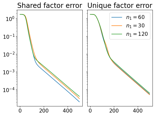
We use synthetic data to examine the numerical convergence of . We generate data according to the model (1), where ${\mathbf{U}^{\star}}_{g}$, ${\mathbf{U}^{\star}}_{(i),l}$, ${\mathbf{V}^{\star}}_{(i),g}$, ${\mathbf{V}^{\star}}_{(i),l}$ are randomly sampled from Gaussian distributions. Then we deflate ${\mathbf{U}^{\star}}_{(i),l}$ to satisfy the requirement ${\mathbf{U}^{\star}}_{g}^{T}{\mathbf{U}^{\star}}_{(i),l}=0$. The noise ${\mathbf{E}^{\star}}_{(i)}$ is set to $0$ to examine the convergence behavior of our algorithm better. We fix $n_{2}=100$ and select $n_{1}\in\{30,60,120\}$ to see the effect of different observation matrix sizes. The ranks of the global and local components are set to $r_{1}=r_{2}=3$, and the number of clients is $N=100$. We run on the generated data with the decision variables $\mathbf{U}_{g}$, $\mathbf{U}_{(i),l}$, $\mathbf{V}_{(i),g}$, $\mathbf{V}_{(i),l}$ initialized as small Gaussian matrices. The errors $\sum_{i=1}^{N}\left\lVert\mathbf{U}_{g,\tau}\mathbf{V}_{(i),g,\tau}^{T}-{\mathbf{U}^{\star}}_{g}{\mathbf{V}^{\star}}_{(i),g}^{T}\right\rVert_{F}^{2}$ and $\sum_{i=1}^{N}\left\lVert\mathbf{U}_{(i),l,\tau}\mathbf{V}_{(i),l,\tau}^{T}-{\mathbf{U}^{\star}}_{(i),l}{\mathbf{V}^{\star}}_{(i),l}^{T}\right\rVert_{F}^{2}$ are calculated in each iteration and plotted as shared feature error and unique feature error in Figure 1. It can be observed that after a few iterations¹¹ 1 The initial sublinear convergence of the algorithm is due to the fact that our initial point does not satisfy the condition of Theorem 3. However, once the iterations reach the basin of attraction of the global solution, the iterations converge linearly., the errors decrease linearly, which is consistent with our theoretical guarantee in Theorem 3.

We also compare with three representative baseline algorithms on the synthetic dataset. To simulate the effects of missing entries, we uniformly randomly remove a subset of entries in each $\mathbf{M}_{(i)}$. Then we run with $\ell^{pse}$, JIVE, RJIVE, and perPCA on the partially observed $\{\mathbf{M}_{(i)}\}$ and calculate the subspace error defined as $\left\lVert\mathbf{P}_{\mathbf{U}_{g}}-\mathbf{P}_{{\mathbf{U}^{\star}}_{g}}\right\rVert_{F}^{2}+\frac{1}{N}\sum_{i=1}^{N}\left\lVert\mathbf{P}_{\mathbf{U}_{(i),l}}-\mathbf{P}_{{\mathbf{U}^{\star}}_{(i),l}}\right\rVert_{F}^{2}$. The missing entries are treated as zero in JIVE, RJIVE, and perPCA. We run the experiments from $3$ different random seeds and calculate the mean and standard deviation of the subspace error. Results are reported in Table. 2.

In Table. 2, has consistently low subspace error, even when the ratio of missing elements is as high as 50%. The result highlights ’s superior ability to recover shared and unique features from incomplete data.

We use an illustrative example in video segmentation to demonstrate the application of . The video comes from a simulated surveillance dataset (Vacavant et al. 2013). In the video, multiple vehicles drive through a roundabout. We uniformly randomly remove $40\%$ pixels to simulate the effects of missing observations. We divide each video frame $i$ into multiple $7\times 7$ patches and flatten these patches into row vectors to construct observation matrix $\mathbf{M}_{(i)}$. Then, we apply to identify the shared and unique signals from the observation matrices with $r_{1}=20$ and $r_{2,(i)}=r_{2}=30$. Naturally, the shared signals will correspond to the stationary components in the video, and unique signals correspond to the changing parts. We reconstruct the frames from the shared and unique signals and plot the results in Figure 2.

The first row of Figure 2 shows $5$ sample frames from the video. They are corrupted as many pixels are missing. The second row plots the reconstructed $\mathbf{U}_{g}\mathbf{V}_{(i),g}^{T}$, one can see that clearly identifies the fine details on the background. The third row of Figure 2 are the reconstructed $\mathbf{U}_{(i),l}\mathbf{V}_{(i),l}^{T}$, which also conspicuously show the moving cars.

As comparisons, we also run benchmark algorithms JIVE, RJIVE, and perPCA on the same dataset with the same data preprocessing procedures. To evaluate the segmentation performance, we calculate the mean squared error (MSE) and the peak signal-to-noise ratio (PSNR) for the recovered foreground and backgrounds. Results are shown in Table 3.

A higher level of quality in the reconstructed background and foreground is typically associated with a lower MSE and a higher PSNR. As indicated in Table 3, it is evident that consistently achieves lower MSE and higher PSNR values for both foreground and background reconstructions in comparison to benchmark algorithms, thus confirming its superior performance.

can also be applied to data from the financial market. As a proof-of-concept, we analyze the daily stock prices of 214 stocks from January 2, 1990 to November 9, 2017. The goal is to understand the time-specific patterns in stock prices. These patterns are often related to abnormal market behaviors and provide insightful information for subsequent trading decisions.

Similar to (Fattahi and Gomez 2021), we use a time window of $30$ days to group the stock prices into different batches, and analyze the common and unique features among these batches. Each batched data matrix $\mathbf{M}_{(i)}$ has dimension $214\times 30$. The unique features represent structural differences in the stock prices in each batch, thus signaling sudden changes in the market. To find the unique features, we apply on the batched data to extract $\mathbf{U}_{(i),l}$’s and $\mathbf{V}_{(i),l}$’s. To measure the “heterogeneity index” in each batch, we calculate the column-wise $\ell_{1}$ norm of the signal matrix $\mathbf{U}_{(i),l}\mathbf{V}_{(i),l}^{T}$ for each $i$. The heterogeneity indices are plotted as the blue curve in Figure 3. To provide better insight, we also plot the SP500 closing prices in the same figure.

From Figure 3, one can observe that almost every significant historical market crash (shown as sudden drops in the orange curve) corresponds to a peak in the heterogeneity index. We also identify $4$ major periods when the heterogeneity index has several large peaks. By comparing these periods with the history of the global financial market (Wikipedia 2023), one can see that A corresponds to the “dot-com bubble”, B corresponds to the “September 11 attack”, C corresponds to “stock market downturn of 2002”, and D corresponds to the “2007-2008 financial crisis and the aftermath”.

The ability to effectively distinguish between shared and unique features is also beneficial in recommender systems. This is exemplified in the MovieLens-100k dataset (Harper and Konstan 2015). The dataset contains $10^{5}$ ratings (1-5) on 1682 movies from 943 users. Additionally, each movie is labeled with genre labels, such as action, adventure, or animation. There are 19 genres in total. Notice that each movie can have more than one genre label. For example, the movie Titanic belongs to both the romance and drama genre.

To characterize the genre information, we first cluster movies into different groups according to the genre labels. Different groups represent different sources. More specifically, for movie $m$, we use multi-hot encoding to create its genre information vector $g_{m}\in\mathbb{R}^{19}$, whose $j$-th element is $1$ if movie $m$ belongs to genre $j$. Next, we normalize $g_{m}$ and use K-means clustering to cluster the normalized $g_{m}$s into $10$ groups. For each group, we construct user-movie rating matrices $\mathbf{M}_{(i)}$. Each $\mathbf{M}_{(i)}$ has 943 rows, and its number of columns is equal to the number of movies in cluster $i$. Thus $\mathbf{M}_{(i)}$ is highly sparse. Then we randomly split each $\Omega_{(i)}$ into $90\%$ training set $\Omega_{(i)}^{train}$ and $10\%$ test set $\Omega_{(i)}^{test}$ and apply with $\ell^{pse}$ on the $\Omega_{(i)}^{train}$.

We use two methods to predict the user ratings on unseen movies: (i) collaborative filtering, which is based on linear model (3), and (ii) auto-encoders, which is based on the nonlinear model (5).

Collaborative filtering The standard collaborative filtering method pools ratings for movies from all genres and exploits matrix completion to extract the low-rank movie features and user features on $\cup_{i}\Omega_{(i)}^{train}$ (Koren et al. 2009). These features can then be leveraged for new rating predictions on unseen movies. Though achieving decent performance, the standard collaborative filtering only finds generic movie features and neglects the genre information. To incorporate the genre information, we apply to the genre-clustered ratings $\mathbf{M}_{(i)}$ to identify both generic features and genre-specific features. The new predictions are given as the entries of $\hat{\mathbf{U}}_{g}\hat{\mathbf{V}}_{(i),g}+\hat{\mathbf{U}}_{(i),l}\hat{\mathbf{V}}_{(i),l}$.

Auto-encoder As discussed in Section 3.2, auto-encoders are nonlinear extensions to matrix factorization models and can potentially encode richer information. The auto-encoders have been employed in the rating prediction tasks and have been shown to outperform collaborative filtering based on linear features (Muller et al. 2018). The standard auto-encoder approach for rating prediction minimizes the following reconstruction loss,

, where $\mathbf{M}^{obs}$ is the observed rating matrix $\mathbf{M}$ padded with zero in all entries outside the training set $\Omega_{train}$. $\mathcal{R}\left(\mathbf{U},\mathbf{V}\right)$ is the regularization term dependent on the architecture of the neural network.

There are numerous works focusing on the architecture of the encoder and decoder network (Zhang et al. 2017; Darban and Valipour 2022; Rashed et al. 2019). Among them, sparsely supported fully connected neural network (SparseFC) (Muller et al. 2018) achieves decent performance. We briefly introduce the main idea of sparse FC for consistency. A standard full-connected neural network consists of multiple layers. Layer $l$ will transform the input $x^{(l-1)}$ to the output $x^{(l)}$ via a linear mapping $W^{(l)}$ followed by a nonlinear activation $\sigma^{(l)}$, i.e., $x^{(l)}=\sigma^{(l)}(W^{(l)}x^{(l-1)})$. A sparse kernel layer chooses a different parametrization of the linear mapping $W^{(l)}$. More specifically, the $j$-th element out the output $x^{(l)}$ is given by,

, where $\alpha_{i}^{(l)}$, $u^{(l)}_{i}$, and $u^{(l)}_{j}$ are trainable parameters. $K$ is a kernel function that can be defined as Gaussian kernel $K(x,y)=\exp\left(-\gamma\left\lVert x-y\right\rVert^{2}\right)$. Intuitively, such parametrization would make the weights $K(u^{(l)}_{i},u^{(l)}_{j})$ sparse. Sparse FC networks are constructed by sequentially applying sparse kernel layers. Because of their superior generalization performance, we use sparse neural networks as the backbones for the encoder and decoder networks $\texttt{Net}_{\mathbf{U}}$ and $\texttt{Net}_{\mathbf{V}}$ in (10). We implement the architecture and pool $\mathbf{M}_{(i)}$ to build $\mathbf{M}$, then solve (10) with AdamW (Loshchilov and Hutter 2019).

As introduced in Section 3.2, we can also employ a heterogeneous version of auto-encoders HAE. More specifically, we use a shared encoder network $\texttt{Net}_{\mathbf{U}_{g}}$ and $10$ genre-specific encoders $\texttt{Net}_{\mathbf{U}_{(i),l}}$ to learn both shared and unique nonlinear embeddings of movies. Then, we use a decoder $\texttt{Net}_{\mathbf{V}}$ to predict user ratings. We still use the sparse FC network as the backbones of the encoders and decoders.

To visualize the embeddings from standard auto-encoders and heterogeneous auto-encoders, we show t-SNE plots of different movie embeddings in Figure 4.

In Figure 4, it is clear that the embeddings from HAE form clusters dependent on the genre, while the embeddings from standard auto-encoders do not have a clear structure. These observations are consistent with our intuition that movies with similar genres should have similar embeddings.

With the fitted models from or HAE, we can predict user ratings on unseen movies. To evaluate the predictive performance, we calculate the predicted ratings on the test set $\Omega_{(i)}^{test}$ and compare it with the ground truth. As the movielens 100k dataset is extensively analyzed in the literature, we also report the RMSE of a few representative benchmark methods detailed as follows,

• •

  Matrix completion (Koren et al. 2009): We implement the standard matrix completion on the pooled rating matrix $\mathbf{M}$ to extract linear features.

• •

  AutoSVD++ (Zhang et al. 2017): AutoSVD++ is a hybrid model combining a variant of biased SVD and a 1-layer fully connected neural network.

• •

  GHRS (Darban and Valipour 2022): Graph-based Hybrid Recommendation System builds user similarity graph based on user ratings and side information, including age and occupation, then clusters users into different groups and uses group features to make predictions on the unseen ratings.

• •

  GraphRec (Rashed et al. 2019): GraphRec is a nonlinear model that uses a neural network to create user and movie embeddings. It also considers the graph-based features from the user similarity graph.

The root mean square error (RMSE) of the prediction on the test set is shown in Table 4. For matrix completion, , Sparse FC, and HAE, we run each experiment from $80$ different random seeds and report the mean and standard deviation. For other methods, we report the performance from the literature.

In Table 4, it is clear that HAE has the lowest test error, suggesting that the heterogeneous features learned by HAE are more accurate in terms of predicting the users’ preferences. Therefore, the genre features bring useful information to the movie ratings prediction.

References

- Bertsekas (1997) D. P. Bertsekas. Nonlinear programming. Journal of the Operational Research Society, 48(3):334–334, 1997.
- Chai et al. (2021) D. Chai, L. Wang, K. Chen, and Q. Yang. Secure federated matrix factorization. IEEE Intelligent Systems, 36(5):11–20, 2021. doi: 10.1109/MIS.2020.3014880.
- Chen et al. (2020) J. Chen, D. Liu, and X. Li. Nonconvex rectangular matrix completion via gradient descent without regularization. IEEE Transactions on Information Theory, 66(9):5806–5841, 2020.
- Curtis and Overton (2012) F. E. Curtis and M. L. Overton. A sequential quadratic programming algorithm for nonconvex, nonsmooth constrained optimization. SIAM Journal on Optimization, 22(2):474–500, 2012.
- Darban and Valipour (2022) Z. Z. Darban and M. H. Valipour. Ghrs: Graph-based hybrid recommendation system with application to movie recommendation. Expert Systems with Applications, 200:116850, 2022.
- Fattahi and Gomez (2021) S. Fattahi and A. Gomez. Scalable inference of sparsely-changing gaussian markov random fields. In M. Ranzato, A. Beygelzimer, Y. Dauphin, P. Liang, and J. W. Vaughan, editors, Advances in Neural Information Processing Systems, volume 34, pages 6529–6541. Curran Associates, Inc., 2021. URL https://proceedings.neurips.cc/paper_files/paper/2021/file/33853141e0873909be88f5c3e6144cc6-Paper.pdf.
- Fattahi and Sojoudi (2020) S. Fattahi and S. Sojoudi. Exact guarantees on the absence of spurious local minima for non-negative rank-1 robust principal component analysis. Journal of machine learning research, 2020.
- Gaynanova and Li (2019) I. Gaynanova and G. Li. Structural learning and integrative decomposition of multi-view data. Biometrics, 75(4):1121–1132, 2019.
- Ge et al. (2017) R. Ge, C. Jin, and Y. Zheng. No spurious local minima in nonconvex low rank problems: A unified geometric analysis. In International Conference on Machine Learning, pages 1233–1242. PMLR, 2017.
- Gemulla et al. (2011) R. Gemulla, E. Nijkamp, P. J. Haas, and Y. Sismanis. Large-scale matrix factorization with distributed stochastic gradient descent. In Proceedings of the 17th ACM SIGKDD international conference on Knowledge discovery and data mining, pages 69–77, 2011.
- Goodfellow et al. (2016) I. Goodfellow, Y. Bengio, and A. Courville. Deep Learning. MIT Press, 2016. http://www.deeplearningbook.org.
- Harper and Konstan (2015) F. M. Harper and J. A. Konstan. The movielens datasets: History and context. Acm transactions on interactive intelligent systems (tiis), 5(4):1–19, 2015.
- Higgins et al. (2017) I. Higgins, L. Matthey, A. Pal, C. Burgess, X. Glorot, M. Botvinick, S. Mohamed, and A. Lerchner. beta-VAE: Learning basic visual concepts with a constrained variational framework. In International Conference on Learning Representations, 2017. URL https://openreview.net/forum?id=Sy2fzU9gl.
- Hong and Luo (2017) M. Hong and Z.-Q. Luo. On the linear convergence of the alternating direction method of multipliers. Mathematical Programming, 162(1-2):165–199, 2017.
- Kontar et al. (2021) R. Kontar, N. Shi, X. Yue, S. Chung, E. Byon, M. Chowdhury, J. Jin, W. Kontar, N. Masoud, M. Nouiehed, et al. The internet of federated things (ioft). IEEE Access, 9:156071–156113, 2021.
- Koren et al. (2009) Y. Koren, R. Bell, and C. Volinsky. Matrix factorization techniques for recommender systems. Computer, 42(8):30–37, 2009. doi: 10.1109/MC.2009.263.
- Lee and Seung (1999) D. D. Lee and H. S. Seung. Learning the parts of objects by non-negative matrix factorization. Nature, 401(6755):788–791, 1999.
- Li et al. (2018a) X. Li, J. Haupt, J. Lu, Z. Wang, R. Arora, H. Liu, and T. Zhao. Symmetry. saddle points, and global optimization landscape of nonconvex matrix factorization. In 2018 Information Theory and Applications Workshop (ITA), pages 1–9, 2018a. doi: 10.1109/ITA.2018.8503215.
- Li et al. (2018b) Y. Li, T. Ma, and H. Zhang. Algorithmic regularization in over-parameterized matrix sensing and neural networks with quadratic activations. In Conference On Learning Theory, pages 2–47. PMLR, 2018b.
- Liang et al. (2023) G. Liang, N. Shi, R. A. Kontar, and S. Fattahi. Personalized dictionary learning for heterogeneous datasets. In Thirty-seventh Conference on Neural Information Processing Systems, 2023. URL https://openreview.net/forum?id=xw6Szwu4xz.
- Lock et al. (2013) E. F. Lock, K. A. Hoadley, J. S. Marron, and A. B. Nobel. Joint and individual variation explained (jive) for integrated analysis of multiple data types. The annals of applied statistics, 7(1):523, 2013.
- Loshchilov and Hutter (2019) I. Loshchilov and F. Hutter. Decoupled weight decay regularization. In International Conference on Learning Representations, 2019. URL https://openreview.net/forum?id=Bkg6RiCqY7.
- Ma et al. (2018) C. Ma, K. Wang, Y. Chi, and Y. Chen. Implicit regularization in nonconvex statistical estimation: Gradient descent converges linearly for phase retrieval and matrix completion. In International Conference on Machine Learning, pages 3345–3354. PMLR, 2018.
- Ma and Fattahi (2022) J. Ma and S. Fattahi. Global convergence of sub-gradient method for robust matrix recovery: Small initialization, noisy measurements, and over-parameterization. arXiv preprint arXiv:2202.08788, 2022.
- Ma et al. (2022) J. Ma, L. Guo, and S. Fattahi. Behind the scenes of gradient descent: A trajectory analysis via basis function decomposition. arXiv preprint arXiv:2210.00346, 2022.
- Muller et al. (2018) L. Muller, J. Martel, and G. Indiveri. Kernelized synaptic weight matrices. In International Conference on Machine Learning, pages 3654–3663. PMLR, 2018.
- Park et al. (2017) D. Park, A. Kyrillidis, C. Carmanis, and S. Sanghavi. Non-square matrix sensing without spurious local minima via the Burer-Monteiro approach. In A. Singh and J. Zhu, editors, Proceedings of the 20th International Conference on Artificial Intelligence and Statistics, volume 54 of Proceedings of Machine Learning Research, pages 65–74. PMLR, 20–22 Apr 2017. URL https://proceedings.mlr.press/v54/park17a.html.
- Park and Lock (2020) J. Y. Park and E. F. Lock. Integrative factorization of bidimensionally linked matrices. Biometrics, 76(1):61–74, 2020.
- Rashed et al. (2019) A. Rashed, J. Grabocka, and L. Schmidt-Thieme. Attribute-aware non-linear co-embeddings of graph features. In Proceedings of the 13th ACM conference on recommender systems, pages 314–321, 2019.
- Sagonas et al. (2017) C. Sagonas, Y. Panagakis, A. Leidinger, and S. Zafeiriou. Robust joint and individual variance explained. In Proceedings of the IEEE Conference on Computer Vision and Pattern Recognition, pages 5267–5276, 2017.
- Shi and Kontar (2024) N. Shi and R. A. Kontar. Personalized pca: Decoupling shared and unique features. Journal of machine learning research, 2024.
- Stöger and Soltanolkotabi (2021) D. Stöger and M. Soltanolkotabi. Small random initialization is akin to spectral learning: Optimization and generalization guarantees for overparameterized low-rank matrix reconstruction. Advances in Neural Information Processing Systems, 34:23831–23843, 2021.
- Sun and Luo (2016) R. Sun and Z.-Q. Luo. Guaranteed matrix completion via non-convex factorization. IEEE Transactions on Information Theory, 62(11):6535–6579, 2016.
- Tu et al. (2016) S. Tu, R. Boczar, M. Simchowitz, M. Soltanolkotabi, and B. Recht. Low-rank solutions of linear matrix equations via procrustes flow. In International Conference on Machine Learning, pages 964–973. PMLR, 2016.
- Vacavant et al. (2013) A. Vacavant, T. Chateau, A. Wilhelm, and L. Lequievre. A benchmark dataset for outdoor foreground/background extraction. In Computer Vision-ACCV 2012 Workshops: ACCV 2012 International Workshops, Daejeon, Korea, November 5-6, 2012, Revised Selected Papers, Part I 11, pages 291–300. Springer, 2013.
- Wang and Fan (2022) B. Wang and J. Fan. Robust matrix completion with heavy-tailed noise. arXiv preprint arXiv:2206.04276, 2022.
- Wikipedia (2023) Wikipedia. List of stock market crashes and bear markets, 2023. URL https://en.wikipedia.org/wiki/List_of_stock_market_crashes_and_bear_markets. [Online; accessed 17-May-2023].
- Wright and Ma (2022) J. Wright and Y. Ma. High-dimensional data analysis with low-dimensional models: Principles, computation, and applications. Cambridge University Press, 2022.
- Yang and Leskovec (2013) J. Yang and J. Leskovec. Overlapping community detection at scale: a nonnegative matrix factorization approach. In Proceedings of the sixth ACM international conference on Web search and data mining, pages 587–596, 2013.
- Yang and Michailidis (2016) Z. Yang and G. Michailidis. A non-negative matrix factorization method for detecting modules in heterogeneous omics multi-modal data. Bioinformatics, 32(1):1–8, 2016.
- Ye and Du (2021) T. Ye and S. S. Du. Global convergence of gradient descent for asymmetric low-rank matrix factorization. Advances in Neural Information Processing Systems, 34:1429–1439, 2021.
- Yu et al. (2016) H.-F. Yu, N. Rao, and I. S. Dhillon. Temporal regularized matrix factorization for high-dimensional time series prediction. Advances in neural information processing systems, 29, 2016.
- Zhang et al. (2017) S. Zhang, L. Yao, and X. Xu. Autosvd++ an efficient hybrid collaborative filtering model via contractive auto-encoders. In Proceedings of the 40th International ACM SIGIR conference on Research and Development in Information Retrieval, pages 957–960, 2017.
- Zhou et al. (2015) G. Zhou, A. Cichocki, Y. Zhang, and D. P. Mandic. Group component analysis for multiblock data: Common and individual feature extraction. IEEE transactions on neural networks and learning systems, 27(11):2426–2439, 2015.
Appendix A The algorithm to solve (5)
In this section, we introduce the detailed algorithm to solve (5). The algorithm uses AdamW (Loshchilov and Hutter 2019) as the backbone to optimize the regularized reconstruction loss (5). To enforce the orthogonality constraint between the shared embeddings and the unique embeddings, we explicitly calculate the projection of the unique embeddings to the subspace spanned by the shared embeddings and remove such projection from the unique embeddings. The pseudo-code is presented in Algorithm 2.
In each iteration of Algorithm 2, we calculate the shared and unique embeddings for each source . For two tensors , the projection operator outputs another tensor. Its -th element is defined as,
, where we use to denote the -th slice of . Intuitively, the projection operator projects each slice of onto the subspace spanned by the column vectors of in the corresponding slice.
The unfolding operator is the inverse of the folding operator . It can be easily implemented via the Rearrange function in pytorch. After the projection step, is orthogonal to . Thus, the orthogonality constraint in (5) is strictly satisfied.
The folding, projection, and unfolding operations are fully differentiable. Hence, after calculating the regularized loss, we can use auto-differentiation packages to take the gradient of the regularized loss with respect to the parameters of the neural network. The gradients are then passed to the AdamW optimizer to update the parameters. After updating all the parameters, the weights for the decoder and for the shared encoder are averaged.
The algorithm repeats for rounds.
Appendix B Proof of Theorem 1
For a matrix , we use or to denote ’s operator norm and to denote its Frobenius norm.
The proof mainly consists of a perturbation analysis of the objective (4) in the main paper. We assume that the loss metric is the square loss throughout this section. We firstly estimate the subspace error of and . Then we estimate the reconstruction errors.
The KKT conditions for the optimal and are,
Considering the constraint , we can solve and as,
Then the objective becomes,
Notice that if and are optimal, we must have and , since we can always use Schmidt-Gram procedure to orthonormalize the columns of and without changing and . Therefore without loss of generality, we consider the problem
By our assumption on the data generation process, and ’s are also feasible. Thus the objective evaluated at and ’s cannot be smaller than the optimal objective,
This is equivalent to