跳到论文正文
W Papers独立论文阅读器 arXiv:2305.17630 论文正文 计算阅读时间 · 0%
引用这篇论文根据当前论文元数据生成,正式投稿前建议核对。


License: arXiv.org perpetual non-exclusive license
arXiv:2305.17630v2 [quant-ph] 08 Jan 2024

Solving quantum optimal control problems using projection operator-based Newton steps

Jieqiu Shao Affiliation: College of Engineering and Applied Science, University of Colorado Boulder, Boulder, Colorado 80309, USA    Mantas Naris Affiliation: College of Engineering and Applied Science, University of Colorado Boulder, Boulder, Colorado 80309, USA    John Hauser Affiliation: College of Engineering and Applied Science, University of Colorado Boulder, Boulder, Colorado 80309, USA    Marco M. Nicotra Affiliation: College of Engineering and Applied Science, University of Colorado Boulder, Boulder, Colorado 80309, USA
August 11, 2026
Abstract

The Quantum PRojection Operator-based Newton method for Trajectory Optimization, a.k.a. Q-PRONTO, is a numerical method for solving quantum optimal control problems. This paper significantly improves prior versions of the quantum projection operator by introducing a regulator that stabilizes the solution estimate at every iteration. This modification is shown to not only improve the convergence rate of the algorithm, but also steer the solver towards better local minima compared to the un-regulated case. Numerical examples showcase how Q-PRONTO can be used to solve multi-input quantum optimal control problems featuring time-varying costs and undesirable populations that ought to be avoided during the transient.

I Introduction

Quantum optimal control is an enabling technology that allows quantum systems to operate at their fullest potential Brif et al. 2010; Dong and Petersen 2010; Altafini and Ticozzi 2012; Glaser et al. 2015. Model-based solvers predominantly rely on the GRadient Ascent Pulse Engineering algorithm (GRAPE) Khaneja et al. 2001; Khaneja et al. 2005 or the Krotov method Sklarz and Tannor 2002; Reich et al. 2012, both of which feature a linear convergence rate, or superlinear in the case of gradient acceleration schemes de Fouquieres et al. 2011; Eitan et al. 2011. In prior work, the authors introduced Q-PRONTO Shao et al. 2022: a Newton-based quantum optimal control solver that can achieve quadratic convergence.

Although Q-PRONTO is a quantum adaptation of the general-purpose Projection Operator-based Newton method for Trajectory Optimization Hauser 2002; Hauser 2003, the prior version Shao et al. 2022 featured a simplified formulation that did not include a regulator. The main contribution of this paper is to augment Q-PRONTO’s projection operator with a regulator term. This improves the numerical stability of the algorithm, thereby boosting its convergence rate by enabling it to take larger steps at each iteration.

In addition to improving the convergence rate of the Q-PRONTO algorithm by introducing the regulator, the paper extends the range of quantum optimal control problems it can address by detailing how to i) perform both phase-sensitive and phase-insensitive state transformations, ii) penalize undesirable states during he transient behavior, iii) handle multiple inputs,iv) use idealized behaviors as an initial guess for the solver, , and v) design quantum gates.

The paper is structured as follows: Section II introduces the quantum control problem and shows how to reformulate it as a real-valued optimal control problem. Section III redevelops the Q-PRONTO formulation in the presence of a possibly non-zero feedback regulator. Section IV details how to design the regulator depending on the control objectives. Section V features three numerical examples: the first illustrates the benefits of using a non-zero feedback gain, the second highlights the novel capabilities of Q-PRONTO, and the third show how to design a quantum gate.

II Problem Statement

The objective of this paper is to develop a numerically efficient algorithm for solving quantum optimal control problems Brif et al. 2010 in the form

min\displaystyle\displaystyle\min~~ 𝒥⁡(|ψ⁡(T)⟩)+∫0Tℓ⁡(|ψ⁡(t)⟩,u⁡(t),t)​𝑑t\displaystyle\displaystyle\mathcal{J}\bigl(\ket{\psi(T)}\bigr)+\int_{0}^{T}\ell\bigl(\ket{\psi(t)},u(t),t\bigr)dt (1a)
s.t.   i​ℏ​|ψ˙​(t)⟩=ℋ⁡(u⁡(t))​|ψ⁡(t)⟩,|ψ⁡(0)⟩=|ψ0⟩,\displaystyle\mathrm{i}\hbar\ket{\dot{\psi}(t)}=\mathcal{H}\bigl(u(t)\bigr)\ket{\psi(t)},\qquad\ket{\psi(0)}=\ket{\psi_{0}},~~~ (1b)

where (1b) is the Shrödinger equation of a closed quantum system governed by the control Hamiltonian ℋ⁡(u)\mathcal{H}(u) and (1a) is a cost function that encapsulates the control objectives. Note that |ψ⁡(t)⟩\ket{\psi(t)} can be interpreted as either a wavefunction or a vector of wavefunctions. As detailed in Section II.3, the latter is useful for quantum gate design. Each component is characterized as follows.

II.1 Schrödinger Equation

Given the unit wavefunction |ψ⟩∈ℂn\ket{\psi}\in\mathbb{C}^{n} and the control input vector u∈ℝmu\in\mathbb{R}^{m}, the Shrödinger equation (1b) is governed by the control Hamiltonian

ℋ⁡(u)=ℋ0+∑j=1mℋj​fj​(uj),\mathcal{H}(u)=\mathcal{H}_{0}+\sum_{j=1}^{m}\mathcal{H}_{j}\,f_{j}(u_{j}), (2)

where ℋ0\mathcal{H}_{0} describes the free evolution of the system, ℋj\mathcal{H}_{j} describes the evolution induced by the jj-th control input, and fj:ℝ→ℝf_{j}\mathrel{\mathop{\mathchar 58\relax}}\mathbb{R}\to\mathbb{R} are class 𝒞2\mathcal{C}^{2} functions that capture possible nonlinearities. To ensure that ‖|ψ⁡(t)⟩‖\|\!\ket{\psi(t)}\!\| is constant, the matrices ℋ0\mathcal{H}_{0}, ℋj\mathcal{H}_{j} are assumed to be Hermitian.

II.2 Cost Function

The cost function (1a) is comprised of a terminal cost 𝒥⁡(|ψ⟩)\mathcal{J}(\ket{\psi}) and an incremental cost ℓ⁡(|ψ⟩,u,t)\ell(\ket{\psi},u,t). The former penalizes deviations between a given objective and the final wavefunction |ψ⁡(T)⟩\ket{\psi(T)}, whereas the latter penalizes undesirable behaviors during the time window t∈[0,T]t\in[0,T]. To ensure the existence and uniqueness of the solution, it is assumed that 𝒥:ℂn→ℝ\mathcal{J}\mathrel{\mathop{\mathchar 58\relax}}\mathbb{C}^{n}\to\mathbb{R} is a class 𝒞2\mathcal{C}^{2} convex function and ℓ:ℂn×ℝm×[0,T]→ℝ\ell\mathrel{\mathop{\mathchar 58\relax}}\mathbb{C}^{n}\times\mathbb{R}^{m}\times[0,T]\to\mathbb{R} is a class 𝒞2\mathcal{C}^{2} function that is convex in |ψ⟩\ket{\psi} and strongly convex in uu for all t∈[0,T]t\in[0,T].

For the reader’s convenience, the following paragraphs provide suitable examples of cost functions when |ψ⟩\ket{\psi} is a single wavefunction. Although these cost functions stem from the ones featured in Brif et al. 2010, they have been manipulated to satisfy the convexity assumption.

Terminal Cost
The terminal cost typically captures the main control objective of the quantum optimal control problem. Indeed, (1) aims to steer the wavefunction from an initial condition |ψ0⟩\ket{\psi_{0}} to a final condition |ψT⟩\ket{\psi_{T}} that, ideally, satisfies 𝒥⁡(|ψT⟩)=0\mathcal{J}(\ket{\psi_{T}})=0. The choice of 𝒥⁡(⋅)\mathcal{J}(\cdot) depends on the global phase that is allowed between the target |ψT⟩\ket{\psi_{T}} and the final wavefunction |ψ⁡(T)⟩\ket{\psi(T)}.

Zero Phase Error: If the global phase error between |ψT⟩\ket{\psi_{T}} and |ψ⁡(T)⟩\ket{\psi(T)} matters, one would typically choose

𝒥⁡(|ψ⁡(T)⟩)=1−Re⁡(⟨ψ⁡(T)|ψT⟩).\mathcal{J}(\ket{\psi(T)})=1-\mathrm{Re}\left(\left\langle{\psi(T)}\middle|{\psi_{T}}\right\rangle\right). (3)

Unfortunately, this function is not convex. However, it can be rewritten as a convex function by noting that, given two unit wavefuctions |ψ⟩\ket{\psi}, |ϕ⟩\ket{\phi}, it is possible to write ⟨ψ|ψ⟩+⟨ϕ|ϕ⟩=2\left\langle{\psi}\middle|{\psi}\right\rangle+\left\langle{\phi}\middle|{\phi}\right\rangle=2 and ⟨ψ|ϕ⟩+⟨ϕ|ψ⟩=2​Re​(⟨ψ|ϕ⟩)\left\langle{\psi}\middle|{\phi}\right\rangle+\left\langle{\phi}\middle|{\psi}\right\rangle=2\,\mathrm{Re}(\left\langle{\psi}\middle|{\phi}\right\rangle). Based on these properties, (3) can be reformulated as

𝒥⁡(|ψ⁡(T)⟩)=12​(⟨ψ⁡(T)|−⟨ψT|)​(|ψ⁡(T)⟩−|ψT⟩),\mathcal{J}(\ket{\psi(T)})=\tfrac{1}{2}\left(\bra{\psi(T)}-\bra{\psi_{T}}\right)\left(\ket{\psi(T)}-\ket{\psi_{T}}\right), (4)

which is a class 𝒞2\mathcal{C}^{2} convex function of |ψ⁡(T)⟩\ket{\psi(T)}.

Arbitrary Phase: If the global phase error between |ψT⟩\ket{\psi_{T}} and |ψ⁡(T)⟩\ket{\psi(T)} does not matter, a suitable choice for the cost function would be the Hilbert-Schmidt distance

𝒥⁡(|ψ⁡(T)⟩)=1−|⟨ψ⁡(T)|ψT⟩|2.\mathcal{J}(\ket{\psi(T)})=1-\left|\left\langle{\psi(T)}\middle|{\psi_{T}}\right\rangle\right|^{2}. (5)

Although this function is also not convex, it can be rewritten as a convex function by noting that ⟨ψ|ψ⟩=1\left\langle{\psi}\middle|{\psi}\right\rangle=1 and |⟨ψ|ϕ⟩|2=⟨ψ|ϕ⟩​⟨ϕ|ψ⟩|\!\left\langle{\psi}\middle|{\phi}\right\rangle\!|^{2}=\left\langle{\psi}\middle|{\phi}\right\rangle\left\langle{\phi}\middle|{\psi}\right\rangle. Based on these properties, (5) can be rewritten (up to a factor 22) as the class 𝒞2\mathcal{C}^{2} convex function

𝒥⁡(|ψ⁡(T)⟩)=12​⟨ψ⁡(T)|​ΓT​|ψ⁡(T)⟩,\mathcal{J}(\ket{\psi(T)})=\tfrac{1}{2}\bra{\psi(T)}\Gamma_{T}\ket{\psi(T)}, (6)

where ΓT=(I−|ψT⟩⟨ψT|)\Gamma_{T}=(I\!-\!\left|{\psi_{T}}\middle\rangle\!\middle\langle{\psi_{T}}\right|) is a positive definite matrix.

Incremental Cost
The incremental cost is an auxiliary term that ensures that the solution is “well behaved” during the time window t∈[0,T]t\in[0,T]. Unless there are specific reasons to penalize the cross-correlation between |ψ⟩\ket{\psi} and uu, the most common incremental cost is

ℓ⁡(|ψ⟩,u,t)=ℓψ​(|ψ⟩,t)+ℓu​(u,t),\ell(\ket{\psi}\!,u,t\big)=\ell_{\psi}(\ket{\psi}\!,t)+\ell_{u}(u,t), (7)

with ℓψ:ℂn×[0,T]→ℝ\ell_{\psi}\!\mathrel{\mathop{\mathchar 58\relax}}\mathbb{C}^{n}\times[0,T]\!\to\!\mathbb{R} convex in |ψ⟩\ket{\psi} for all t∈[0,T]t\in[0,T] and ℓu:ℝm×[0,T]→ℝ\ell_{u}\!\mathrel{\mathop{\mathchar 58\relax}}\mathbb{R}^{m}\times[0,T]\!\to\!\mathbb{R} strongly convex in uu for all t∈[0,T]t\in[0,T] to ensure that u⁡(t)u(t) does not grow unbounded.

Control Effort: A typical choice for the incremental input cost is the class 𝒞2\mathcal{C}^{2} strongly convex function

ℓu​(u,t)=12​uT​ℛ​(t)​u,\ell_{u}(u,t)=\tfrac{1}{2}u^{T}\mathcal{R}(t)\,u, (8)

where ℛ⁡(t)>0,∀t∈[0,T]\mathcal{R}(t)>0,~\forall t\in[0,T] is a (potentially time-varying) symmetric matrix that penalizes excessive utilization of the control input.

Undesirable Populations: To penalize the population in an undesirable subspace |φ⟩\ket{\varphi}, it is possible to assign the incremental wavefunction cost

ℓψ​(|ψ⟩,t)=12​𝔮​(t)​⟨ψ|​Γ¯φ​|ψ⟩\ell_{\psi}(\ket{\psi},t)=\tfrac{1}{2}\mathfrak{q}(t)\bra{\psi}\overline{\Gamma}_{\varphi}\ket{\psi} (9)

where 𝔮⁡(t)\mathfrak{q}(t) is a is a (potentially time-varying) penalty weight and Γ¯φ=|φ⟩⟨φ|\overline{\Gamma}_{\varphi}=\left|{\varphi}\middle\rangle\!\middle\langle{\varphi}\right| is a positive definite matrix used to compute the projection of |ψ⟩\ket{\psi} onto |φ⟩\ket{\varphi}.

No Penalties: If the wavefunction is allowed to evolve freely during the control period t∈[0,T]t\in[0,T], the common choice for the incremental wavefunction cost is simply

ℓψ​(|ψ⟩,t)=0.\ell_{\psi}(\ket{\psi},t)=0. (10)

II.3 Quantum Gate Design

The optimal control problem (1) can be used to design quantum gates by interpreting |ψ⁡(t)⟩\ket{\psi(t)} as a vector of orthonormal wavefunctions |ψi​(t)⟩\ket{\psi_{i}(t)} subject to the same control hamiltonian ℋψ​(u)\mathcal{H}_{\psi}(u). Given a target unitary UU, let |Ui⟩\ket{U_{i}} denote its i−i-th column and let |ei⟩\ket{e_{i}} be the ii-th column of the identity matrix. Then, designing a quantum gate is equivalent to finding a u⁡(t)u(t) that simultaneously drives each element of the orthonormal basis from the initial condition |ei⟩\ket{e_{i}} to the target |Ui⟩\ket{U_{i}}. This can be achieved as follows.

Schrödinger Equation
Since each element of the orthonormal basis evolves under the same control Hamiltonian Hψ​(u)H_{\psi}(u) starting from different initial conditions, (1b) can be rewritten as

i​ℏ​|ψ˙i​(t)⟩=ℋψ​(u⁡(t))​|ψi​(t)⟩,|ψi​(0)⟩=|ei⟩,\mathrm{i}\hbar\ket{\dot{\psi}_{i}(t)}=\mathcal{H}_{\psi}\bigl(u(t)\bigr)\ket{\psi_{i}(t)},\qquad\ket{\psi_{i}(0)}=\ket{e_{i}}, (11)

for i=1,…,ni=1,\ldots,n, where nn is the size of the unitary UU. To do so, it is sufficient to define |ψ⟩\ket{\psi} as a column vector of all the |ψi⟩\ket{\psi_{i}} and ℋ⁡(u)=In⊗ℋψ​(u)\mathcal{H}(u)=I_{n}\otimes\mathcal{H}_{\psi}(u), where InI_{n} is the identity matrix of size nn and ⊗\otimes is the Kronecker product.

Terminal Cost
Since the relative phase between orthonormal basis vectors is crucial to the definition of a unitary, it is best to use the “zero phase error” terminal cost

𝒥⁡(|ψ⁡(T)⟩)=12​∑i=1n‖|ψi​(T)⟩−|Ui⟩‖2.\mathcal{J}(\ket{\psi(T)})=\tfrac{1}{2}\sum_{i=1}^{n}\left\|\ket{\psi_{i}(T)}-\ket{U_{i}}\right\|^{2}. (12)

Note that it is possible to design partial unitary transforms by omitting terminal costs associated to basis vectors that are considered irrelevant. An example for this is given in Section V.3.

Incremental Cost
The incremental cost can be chosen as

ℓ⁡(|ψ⟩,u,t)=ℓu​(u,t)+∑i=1nℓi​(|ψi⟩,t),\ell(\ket{\psi}\!,u,t\big)=\ell_{u}(u,t)+\sum_{i=1}^{n}\ell_{i}(\ket{\psi_{i}}\!,t), (13)

where each cost ℓi​(|ψi⟩,t)\ell_{i}(\ket{\psi_{i}}\!,t) can be used to penalize the specific trajectory taken by each basis vector |ψi​(t)⟩\ket{\psi_{i}(t)}.

II.4 Equivalent Formulations

Given the Schrödinger equation and a suitable cost function, the final step for implementing PRONTO is to reformulate the complex-valued optimal control problem (1) into the real-valued optimal control problem

min\displaystyle\displaystyle\min\quad m⁡(x⁡(T))+∫0Tl⁡(x⁡(t),u⁡(t),t)​𝑑t\displaystyle\displaystyle m(x(T))+\int_{0}^{T}l(x(t),u(t),t)dt (14a)
s.t. x˙​(t)=H⁡(u⁡(t))​x​(t),x⁡(0)=x0,\displaystyle\dot{x}(t)=H(u(t))\,x(t),\qquad x(0)=x_{0}, (14b)

where x⁡(t)∈ℝ2​nx(t)\in\mathbb{R}^{2n} is the new state variable. As detailed in Appendix A, this can be achieved without any loss of generality by applying the bijective mapping

x=[Re⁡(|ψ⟩)Im⁡(|ψ⟩)],|ψ⟩=[I​i​I]​x,x=\begin{bmatrix}\mathrm{Re}(\ket{\psi})\\ \mathrm{Im}(\ket{\psi})\end{bmatrix},\qquad\ket{\psi}=[\,I~~\mathrm{i}I\,]x, (15)

where II is an identity matrix of size nn. The real-valued optimal control problem (14) is also equivalent to the Banach space optimization problem

minξ∈𝒯⁡h⁡(ξ),\min_{\xi\in\mathcal{T}}~h(\xi), (16)

where ξ=[x⁡(t),u⁡(t)]\xi=[x(t),u(t)] is a state-and-input trajectory pair,

h⁡(ξ)=m⁡(x⁡(T))+∫0Tl⁡(x⁡(t),u⁡(t),t)​𝑑t,h(\xi)=m(x(T))+\int_{0}^{T}l(x(t),u(t),t)dt, (17)

is the cost functional, and

𝒯={ξ|x˙(t)=ℋ(u(t))x(t),x(0)=x0},\mathcal{T}=\{\xi~|~\dot{x}(t)=\mathcal{H}(u(t))\,x(t),~~x(0)=x_{0}\},\vskip 3.0pt (18)

is the trajectory manifold. The main interest in having the three equivalent formulations (1), (14), and (16) is that they each provide a slightly different insight onto the same problem.

III PRONTO for Quantum Systems

As detailed in Shao et al. 2022, the idea behind Q-PRONTO is to turn the constrained optimization problem (16) into an unconstrained optimization problem

min⁡g⁡(η),\min~g(\eta), (19)

where η=[α⁡(t),μ⁡(t)]\eta=[\alpha(t),\mu(t)] is a pair of state-and-input curves that may not belong to the trajectory manifold 𝒯\mathcal{T}. This is achieved by defining

g⁡(η)=h⁡(𝒫⁡(η)),g(\eta)=h(\mathcal{P}(\eta)), (20)

where 𝒫⁡(η)\mathcal{P}(\eta) is an operator that projects any η\eta onto the manifold 𝒯\mathcal{T}. This paper improves the convergence rate of (Shao et al. 2022, Algorithm 1) by implementing a projection operator that relies not only on the input curve μ⁡(t)\mu(t), but also on the state curve α⁡(t)\alpha(t). The updated method is detailed in the new algorithm provided in Appendix B.

The following subsections introduce the new projection operator and show how it can be used to compute the Newton descent direction. For the sake of brevity, algorithmic elements that remain unchanged with respect to Shao et al. 2022, i.e., the quasi-Newton step (lines 14–17) and the use of the Armijo step (lines 24–28) are not detailed in this paper.

III.1 The Projection Operator

Based on the original PRONTO formulation Hauser 2002; Hauser 2003, given ξ=[x⁡(t),u⁡(t)]\xi=[x(t),u(t)] and η=[α⁡(t),μ⁡(t)]\eta=[\alpha(t),\mu(t)], the projection ξ=𝒫⁡(η)\xi=\mathcal{P}(\eta) is obtained by solving the differential equation

{x˙(t)=H(u(t))x(t),x(0)=x0,u⁡(t)=μ⁡(t)−Kr​(t)​(x⁡(t)−α⁡(t)),\left\{\begin{array}[]{l}\dot{x}(t)=H(u(t))\,x(t),\qquad\qquad\qquad~~x(0)=x_{0},\\ u(t)=\mu(t)-K_{r}(t)(x(t)-\alpha(t)),\end{array}\right. (21)

where the regulator Kr​(t)K_{r}(t) is a time-varying feedback gain designed to ensure that trajectory x⁡(t)x(t) tracks the curve α⁡(t)\alpha(t) as closely as possible. By construction, this operator satisfies the following properties

  • •

    Any pair of state-and-input curves η\eta is mapped onto the trajectory manifold, i.e., 𝒫⁡(η)∈𝒯,∀η\mathcal{P}(\eta)\in\mathcal{T},~\forall\eta;

  • •

    Any ξ\xi that is already in the trajectory manifold remains unaffected, i.e. 𝒫⁡(ξ)=ξ,∀ξ∈𝒯\mathcal{P}(\xi)=\xi,~\forall\xi\in\mathcal{T}.

The design of Kr​(t)≠0K_{r}(t)\neq 0 is addressed in Section IV. For the case Kr​(t)=0K_{r}(t)=0 the reader is referred to Shao et al. 2022.

In view of implementing a Newton descent method, the remainder of this section will compute the first and second order approximations of the projection operator.

First Order Approximation
Given ξ∈𝒯\xi\in\mathcal{T}, the first order approximation of 𝒫⁡(ξ)\mathcal{P}(\xi) along a general direction γ\gamma yields ζ=D​𝒫​(ξ)∘γ\zeta=D\mathcal{P}(\xi)\circ\gamma, where the curve ζ=[z⁡(t),v⁡(t)]\zeta=[z(t),v(t)] is obtained from γ=[β⁡(t),ν⁡(t)]\gamma=[\beta(t),\nu(t)] by solving the differential equation

{z˙(t)=Aξ(t)z(t)+Bξ(t)v(t),z(0)=0,v⁡(t)=ν⁡(t)−Kr​(t)​(z⁡(t)−β⁡(t)),\left\{\begin{array}[]{l}\dot{z}(t)=A_{\xi}(t)z(t)+B_{\xi}(t)v(t),\qquad\quad z(0)=0,\\ v(t)=\nu(t)-K_{r}(t)(z(t)-\beta(t)),\end{array}\right. (22)

with

Aξ​(t)=H⁡(u⁡(t)),\displaystyle A_{\xi}(t)=H(u(t)), (23a)
Bξ​(t)=[∂H∂u1​x​(t)…∂H∂um​x​(t)],\displaystyle B_{\xi}(t)=\displaystyle\begin{bmatrix}\frac{\partial H}{\partial u_{1}}x(t)&\ldots&\frac{\partial H}{\partial u_{m}}x(t)\end{bmatrix}, (23b)

representing to the first Fréchet derivative of H⁡(u)​xH(u)x. With some abuse of notation, we refer to [Ak​(t),Bk​(t)][A_{k}(t),B_{k}(t)] as (23) evaluated in ξk=[xk​(t),uk​(t)]\xi_{k}=[x_{k}(t),u_{k}(t)]. An interesting property of the projection operator is that (22) acts as a projection of the curve γ\gamma onto the tangent space of the trajectory manifold

Tξ𝒯={ζ|z˙(t)=Aξ(t)z(t)+Bξ(t)v(t),z(0)=0}.T_{\xi}\mathcal{T}=\{\zeta~|~\dot{z}(t)=A_{\xi}(t)z(t)+B_{\xi}(t)v(t),z(0)=0\}. (24)

Indeed, ∀ξ∈𝒯\forall\xi\in\mathcal{T}, it follows that

D​𝒫​(ξ)∘γ\displaystyle D\mathcal{P}(\xi)\circ\gamma ∈\displaystyle\in Tξ​𝒯,∀γ,\displaystyle T_{\xi}\mathcal{T},\qquad\forall\gamma, (25a)
D​𝒫​(ξ)∘ζ\displaystyle D\mathcal{P}(\xi)\circ\zeta =\displaystyle= ζ,∀ζ∈Tξ​𝒯.\displaystyle\zeta,\qquad\quad~\forall\zeta\in T_{\xi}\mathcal{T}. (25b)

Second Order Approximation
Given ξ∈𝒯\xi\in\mathcal{T} and ζ∈Tξ​𝒯\zeta\in T_{\xi}\mathcal{T}, the second order approximation of 𝒫⁡(ξ)\mathcal{P}(\xi) yields ω=D2​𝒫​(ξ)∘(ζ,ζ)\omega=D^{2}\mathcal{P}(\xi)\circ(\zeta,\zeta), where ω=[y⁡(t),w⁡(t)]\omega=[y(t),w(t)] is obtained from the curve ζ=[z⁡(t),v⁡(t)]\zeta=[z(t),v(t)] by solving the differential equation

{y˙​(t)=Aξ​(t)​y​(t)+Bξ​(t)​w​(t)+Λξ​(t|ζ)w⁡(t)=−Kr​(t)​y​(t),\left\{\begin{array}[]{l}\dot{y}(t)=A_{\xi}(t)y(t)+B_{\xi}(t)w(t)+\Lambda_{\xi}(t|\zeta)\\ w(t)=-K_{r}(t)y(t),\end{array}\right. (26)

with y⁡(0)=0y(0)=0, where

Λξ​(t|ζ)=2∑i=1m∂H∂ui​vi​(t)​z​(t)+∑i=1m[∂2H∂u1​∂ui​x​(t)…∂2H∂um​∂ui​x​(t)]​vi​(t)​v​(t),\begin{array}[]{rl}\Lambda_{\xi}(t|\zeta)=2&\!\!\displaystyle\sum_{i=1}^{m}\frac{\partial H}{\partial u_{i}}v_{i}(t)z(t)\\ +&\!\!\displaystyle\sum_{i=1}^{m}\begin{bmatrix}\frac{\partial^{2}H}{\partial u_{1}\partial u_{i}}x(t)&\ldots&\frac{\partial^{2}H}{\partial u_{m}\partial u_{i}}x(t)\end{bmatrix}v_{i}(t)v(t),\\ \end{array}

is the first order approximation of Aξ​(t)​z​(t)+Bξ​(t)​v​(t)A_{\xi}(t)z(t)+B_{\xi}(t)v(t), linearized around ξ\xi and evaluated in the direction ζ\zeta.

III.2 Newton Descent

Given a solution estimate ξk∈𝒯\xi_{k}\in\mathcal{T}, it is possible to compute a local (i.e. ζ∈Tξ​𝒯\zeta\in T_{\xi}\mathcal{T}) quadratic approximation of the cost function g⁡(η)g(\eta) by defining η=ξk+ζ\eta=\xi_{k}+\zeta and performing the second order expansion

g⁡(η)−g⁡(ξk)≈D​g​(ξk)∘ζ+12​D2​g​(ξk)∘(ζ,ζ).g(\eta)-g(\xi_{k})\approx Dg(\xi_{k})\circ\zeta+\frac{1}{2}D^{2}g(\xi_{k})\circ(\zeta,\zeta). (27)

As a result, the solution to (19) can be computed by performing the Newton step ηk=ξk+ζk\eta_{k}=\xi_{k}+\zeta_{k}, where the local update ζk\zeta_{k} is obtained by solving the linear-quadratic optimal control problem

minζ∈Tξk​𝒯⁡D​g​(ξk)∘ζ+12​D2​g​(ξk)∘(ζ,ζ).\min_{\zeta\in T_{\xi_{k}}\!\!\mathcal{T}}~Dg(\xi_{k})\circ\zeta+\frac{1}{2}D^{2}g(\xi_{k})\circ(\zeta,\zeta). (28)

The solution to (16) can thus be computed using the projected Newton step

ξk+1=𝒫⁡(ξk+ζk),\xi_{k+1}=\mathcal{P}(\xi_{k}+\zeta_{k}), (29)

The following subsections derive the first and second Fréchet derivative terms D​gDg and D2​gD^{2}g.

Linear Terms
Since g⁡(η)=h⁡(𝒫⁡(η))g(\eta)=h(\mathcal{P}(\eta)), it follows from the chain rule and the properties of the projection operator that

D​g​(ξk)∘ζ=D​h​(𝒫⁡(ξk))∘D​𝒫​(ξk)∘ζ=D​h​(ξk)∘ζ.Dg(\xi_{k})\circ\zeta=Dh(\mathcal{P}(\xi_{k}))\circ D\mathcal{P}(\xi_{k})\circ\zeta=Dh(\xi_{k})\circ\zeta. (30)

Evaluating the first Fréchet derivative of the cost (17) in ξk=[xk​(t),uk​(t)]\xi_{k}=[x_{k}(t),u_{k}(t)] and composing it with ζ=[z⁡(t),v⁡(t)]\zeta=[z(t),v(t)] leads to

D​h​(ξk)∘ζ=πk​z​(T)+∫0Tqk​(t)​z​(t)+rk​(t)​v​(t)​𝑑τ,Dh(\xi_{k})\circ\zeta=\pi_{k}z(T)+\!\!\int_{0}^{T}q_{k}(t)z(t)+r_{k}(t)v(t)d\tau, (31)

with

πk\displaystyle\pi_{k} =\displaystyle= ∇xm​(xk​(T)),\displaystyle\nabla_{x}m(x_{k}(T)), (32a)
qk​(t)\displaystyle q_{k}(t) =\displaystyle= ∇xl​(xk​(t),uk​(t),t),\displaystyle\nabla_{x}l(x_{k}(t),u_{k}(t),t), (32b)
rk​(t)\displaystyle r_{k}(t) =\displaystyle= ∇ul​(xk​(t),uk​(t),t).\displaystyle\nabla_{u}l(x_{k}(t),u_{k}(t),t). (32c)

Quadratic Terms
Since g⁡(η)=h⁡(𝒫⁡(η))g(\eta)=h(\mathcal{P}(\eta)), it follows from the chain rule and the properties of the projection operator that

D2​g​(ξk)∘(ζ,ζ)=D2​h​(𝒫⁡(ξk))∘(D​𝒫​(ξk)∘ζ,D​𝒫​(ξk)∘ζ)+Dh(𝒫(ξk))∘D2𝒫(ξk)∘(ζ,ζ)=D2​h​(ξk)∘(ζ,ζ)+D​h​(ξk)∘ω.\begin{array}[]{rl}D^{2}g(\xi_{k})\!\circ\!(\zeta,\zeta)=&\!D^{2}h(\mathcal{P}(\xi_{k}))\!\circ\!(D\mathcal{P}(\xi_{k})\!\circ\!\zeta,D\mathcal{P}(\xi_{k})\!\circ\!\zeta)\\ &\!\!\!\!+\,Dh(\mathcal{P}(\xi_{k}))\!\circ\!D^{2}\mathcal{P}(\xi_{k})\!\circ\!(\zeta,\zeta)\\ =&\!D^{2}h(\xi_{k})\circ(\zeta,\zeta)+\,Dh(\xi_{k})\circ\omega.\end{array}

Evaluating the second Fréchet derivative of (17) and composing it with ζ=[z⁡(t),v⁡(t)]\zeta=[z(t),v(t)] leads to

D2​h​(ξk)∘(ζ,ζ)=z​(T)T​Πk​z​(T)+…∫0T[z⁡(t)v⁡(t)]T​[Q¯k​(t)S¯k​(t)S¯kT​(t)R¯k​(t)]​[z⁡(t)v⁡(t)]​dt,\begin{array}[]{rl}D^{2}h(\xi_{k})\circ(\zeta,\zeta)=&z(T)^{T}\Pi_{k}z(T)+\ldots\\ &\displaystyle\int_{0}^{T}\!\begin{bmatrix}z(t)\\ v(t)\end{bmatrix}^{\!T}\!\!\begin{bmatrix}\bar{Q}_{k}(t)&\bar{S}_{k}(t)\\ \bar{S}_{k}^{T}(t)&\bar{R}_{k}(t)\end{bmatrix}\!\!\begin{bmatrix}z(t)\\ v(t)\end{bmatrix}dt,\end{array}

with

Πk\displaystyle\Pi_{k} =\displaystyle= ∇x​x2m​(xk​(T)),\displaystyle\nabla^{2}_{xx}m(x_{k}(T)), (33a)
Q¯k​(t)\displaystyle\bar{Q}_{k}(t) =\displaystyle= ∇x​x2l​(xk​(t),uk​(t),t),\displaystyle\nabla^{2}_{xx}l(x_{k}(t),u_{k}(t),t), (33b)
S¯k​(t)\displaystyle\bar{S}_{k}(t) =\displaystyle= ∇x​u2l​(xk​(t),uk​(t),t),\displaystyle\nabla^{2}_{xu}l(x_{k}(t),u_{k}(t),t), (33c)
R¯k​(t)\displaystyle\bar{R}_{k}(t) =\displaystyle= ∇u​u2l​(xk​(t),uk​(t),t).\displaystyle\nabla^{2}_{uu}l(x_{k}(t),u_{k}(t),t). (33d)

As for the other term, the composition of D​h​(ξk)Dh(\xi_{k}) with ω=[y⁡(t),w⁡(t)]\omega=[y(t),w(t)] yields

D​h​(ξk)∘ω=πk​y​(T)+∫0Tqk​(t)​y​(t)+rk​(t)​w​(t)​𝑑τ.Dh(\xi_{k})\circ\omega=\pi_{k}y(T)+\!\!\int_{0}^{T}q_{k}(t)y(t)+r_{k}(t)w(t)d\tau. (34)

Unfortunately, this equation does not feature an explicit dependency on the optimization variable ζ\zeta. To overcome this challenge, consider the state transition matrix Φ⁡(t,τ)\Phi(t,\tau) satisfying

Φ˙​(t,τ)=(A⁡(t)−B⁡(t)​Kr​(t))​Φ​(t,τ).\dot{\Phi}(t,\tau)=(A(t)-B(t)K_{r}(t))\Phi(t,\tau). (35)

Then, the solution to (26) is

y⁡(t)=∫0tΦ⁡(t,τ)​Λξ​(τ|ζ)​𝑑s.y(t)=\int_{0}^{t}\Phi(t,\tau)\Lambda_{\xi}(\tau|\zeta)ds. (36)
minπk​z​(T)+12​z​(T)​Πk​z​(T)+∫0T[qk​(t)​rk​(t)]​[z⁡(t)v⁡(t)]+12​[z⁡(t)v⁡(t)]T​[Qk​(t)Sk​(t)SkT​(t)Rk​(t)]​[z⁡(t)v⁡(t)]​𝑑ts.t.z˙(t)=Ak(t)z(t)+Bk(t)v(t),z(0)=0,\begin{array}[]{rl}\min&\displaystyle\pi_{k}z(T)+\frac{1}{2}z(T)\Pi_{k}z(T)+\displaystyle\int_{0}^{T}\begin{bmatrix}q_{k}(t)~~r_{k}(t)\end{bmatrix}\begin{bmatrix}z(t)\\ v(t)\end{bmatrix}+\frac{1}{2}\begin{bmatrix}z(t)\\ v(t)\end{bmatrix}^{\!T}\!\begin{bmatrix}Q_{k}(t)&S_{k}(t)\\ S_{k}^{T}(t)&R_{k}(t)\end{bmatrix}\begin{bmatrix}z(t)\\ v(t)\end{bmatrix}dt\\ \\ \textrm{s.t.}&\dot{z}(t)=A_{k}(t)z(t)+B_{k}(t)v(t),\qquad\qquad z(0)=0,\end{array} (37)

Since w⁡(t)=−Kr​(t)​y​(t)w(t)=-K_{r}(t)y(t), equation (34) becomes

D​h​(ξk)∘ω=πk​y​(T)+∫0T(qk​(t)−rk​(t)​Kr​(t))​y​(t)​𝑑t=πk​y​(T)+∫0T∫0t(qk​(t)−rk​(t)​Kr​(t))​Φ​(t,τ)​Λξ​(τ|ζ)​𝑑τ​𝑑t=πk​y​(T)+∫0T∫sT(qk​(t)−rk​(t)​Kr​(t))​Φ​(t,τ)​Λξ​(τ|ζ)​𝑑t​𝑑τ=∫0TχkT​(τ)​Λξ​(τ|ζ)​dτ,\begin{array}[]{l}\displaystyle Dh(\xi_{k})\circ\omega=\pi_{k}y(T)+\int_{0}^{T}\!\!\!\bigl(q_{k}(t)-r_{k}(t)K_{r}(t)\bigr)\,y(t)dt\\ \displaystyle=\pi_{k}y(T)\!+\!\int_{0}^{T}\!\!\!\!\int_{0}^{t}\!\!\!\bigl(q_{k}(t)\!-\!r_{k}(t)K_{r}(t)\bigr)\Phi(t,\tau)\Lambda_{\xi}(\tau|\zeta)d\tau\,dt\\ \displaystyle=\pi_{k}y(T)\!+\!\int_{0}^{T}\!\!\!\!\int_{s}^{T}\!\!\!\bigl(q_{k}(t)\!-\!r_{k}(t)K_{r}(t)\bigr)\Phi(t,\tau)\Lambda_{\xi}(\tau|\zeta)dt\,d\tau\\ \displaystyle=\int_{0}^{T}\chi_{k}^{T}(\tau)\Lambda_{\xi}(\tau|\zeta)d\tau,\end{array}

where

χkT​(τ)=πk​Φ​(T,τ)+∫τT(qk​(t)−rk​(t)​Kr​(t))​Φ​(t,τ)​𝑑t\chi_{k}^{T}(\tau)=\pi_{k}\Phi(T,\tau)+\int_{\tau}^{T}(q_{k}(t)-r_{k}(t)K_{r}(t))\Phi(t,\tau)dt

is an adjoint variable that evolves backwards in time. Due to the properties of state transition matrices, χk​(t)\chi_{k}(t) can now be obtained by solving the differential equation

−χ˙k=(Ak−Bk​Kr)T​χk+(qk−rk​Kr)T,-\dot{\chi}_{k}=(A_{k}-B_{k}K_{r})^{T}\chi_{k}+(q_{k}-r_{k}K_{r})^{T}\!\!\!, (38)

with final conditions χ⁡(T)=πk\chi(T)=\pi_{k}.

Remark 1

Given Kr​(t)=0K_{r}(t)=0, the adjoint dynamics (38) reduce to the co-state dynamics featured in the Krotov method (Goerz et al. 2019, Eq. (30)), i.e., −χ˙k=AkT​χk+qkT-\dot{\chi}_{k}=A_{k}^{T}\chi_{k}+q_{k}^{T}. As such, the adjoint variable χk​(t)\chi_{k}(t) can be interpreted as a co-state that has been stabilized by the regulator Kr​(t)K_{r}(t).

The direct dependency from ζ=[z⁡(t),v⁡(t)]\zeta=[z(t),v(t)] is then shown to be

χkT​(t)​Λξ​(t|ζ)=[z⁡(t)v⁡(t)]T​[0S~k​(t)S~kT​(t)R~k​(t)]​[z⁡(t)v⁡(t)],\chi_{k}^{T}(t)\Lambda_{\xi}(t|\zeta)=\!\begin{bmatrix}z(t)\\ v(t)\end{bmatrix}^{\!T}\!\!\begin{bmatrix}0&\tilde{S}_{k}(t)\\ \tilde{S}_{k}^{T}(t)&\tilde{R}_{k}(t)\end{bmatrix}\!\!\begin{bmatrix}z(t)\\ v(t)\end{bmatrix},

with

S~k​(t)=[∂H∂ui​χk​(t)…∂H∂um​χk​(t)],R~k​(t)=[χkT​(t)​H11​(t)​xk​(t)…χkT​(t)​Hm​1​(t)​xk​(t)⋱χkT​(t)​H1​m​(t)​xk​(t)…χkT​(t)​Hm​m​(t)​xk​(t)],\begin{array}[]{rl}\tilde{S}_{k}(t)&=\displaystyle\begin{bmatrix}\frac{\partial H}{\partial u_{i}}\chi_{k}(t)&\ldots&\frac{\partial H}{\partial u_{m}}\chi_{k}(t)\end{bmatrix},\\ \\ \tilde{R}_{k}(t)&=\displaystyle\begin{bmatrix}\chi_{k}^{T}(t)H_{11}(t)x_{k}(t)&\ldots&\chi_{k}^{T}(t)H_{m1}(t)x_{k}(t)\\ \vdots&\ddots&\vdots\\ \chi_{k}^{T}(t)H_{1m}(t)x_{k}(t)&\ldots&\chi_{k}^{T}(t)H_{mm}(t)x_{k}(t)\end{bmatrix},\end{array}

and Hi​j​(t)=∂2H∂ui​∂ujH_{ij}(t)=\frac{\partial^{2}H}{\partial u_{i}\partial u_{j}}. As a result, the evaluation of (28) leads to the Linear-Quadratic Optimal Control Problem (LQ-OCP) in equation (37), with

Qk​(t)\displaystyle Q_{k}(t) =\displaystyle= Q¯k​(t),\displaystyle\bar{Q}_{k}(t), (39a)
Sk​(t)\displaystyle S_{k}(t) =\displaystyle= S¯k​(t)+S~k​(t),\displaystyle\bar{S}_{k}(t)+\tilde{S}_{k}(t), (39b)
Rk​(t)\displaystyle R_{k}(t) =\displaystyle= R¯k​(t)+R~k​(t).\displaystyle\bar{R}_{k}(t)+\tilde{R}_{k}(t). (39c)

The main interest in the LQ-OCP (37) is that its solution can be computed explicitly Anderson and Moore 2007. To do so, we first solve the Differential Riccati Equation

{−P˙=AkT​P+P​Ak−KoT​Rk​Ko+Qk,−p˙=(Ak−Bk​Ko)T​p−KoT​rkT+qkT,Ko=Rk−1​(BkT​P+SkT),vo=Rk−1​(BkT​p+rkT),\left\{\begin{array}[]{rll}-\dot{P}=&A^{T}_{k}P\!+\!PA_{k}-K_{o}^{T}R_{k}K_{o}+Q_{k},\\ -\dot{p}=&(A_{k}-B_{k}K_{o})^{T}p-K_{o}^{T}r_{k}^{T}+q_{k}^{T},\\ K_{o}=&R^{-1}_{k}(B_{k}^{T}P+S_{k}^{T}),\\ v_{o}=&R_{k}^{-1}(B^{T}_{k}p+r_{k}^{T}),\end{array}\right. (40)

with final conditions P⁡(T)=ΠkP(T)\!=\!\Pi_{k} and p⁡(T)=πkp(T)=\pi_{k}. Then, the update ζk\zeta_{k} can be obtained by solving

{z˙k​(t)=Ak​(t)​zk​(t)+Bk​(t)​vk​(t),z⁡(0)=0,vk​(t)=−vo​(t)−Ko​(t)​zk​(t).\left\{\begin{array}[]{rll}\dot{z}_{k}(t)=&A_{k}(t)z_{k}(t)+B_{k}(t)v_{k}(t),&z(0)=0,\\ v_{k}(t)=&-v_{o}(t)-K_{o}(t)z_{k}(t).\end{array}\right. (41)

Additional algorithmic considerations, such as using the Armijo rule to limit the Newton step size, or replacing (Qk,Sk,Rk)(Q_{k},S_{k},R_{k}) with (Q¯k,S¯k,R¯k)(\bar{Q}_{k},\bar{S}_{k},\bar{R}_{k}) whenever (37) does not admit a solution, are detailed in prior work Shao et al. 2022.

IV Regulator Design

Since the projection operator (21) is defined up to a time-varying feedback gain Kr​(t)K_{r}(t), the objective of this section is to design a regulator such that the trajectory ξ=𝒫⁡(η)\xi=\mathcal{P}(\eta) tracks η\eta “as closely as possible”. To provide a more formal metric for success, consider the error coordinates Δ​x​(t)=x⁡(t)−α⁡(t)\Delta x(t)=x(t)-\alpha(t) and Δ​u​(t)=u⁡(t)−μ⁡(t)\Delta u(t)=u(t)-\mu(t). Then, given arbitrary cost matrices Qr​(t)≥0Q_{r}(t)\geq 0, Rr​(t)>0R_{r}(t)>0, and Πr≥0\Pi_{r}\geq 0, the optimal feedback gain Kr​(t)K_{r}(t) can be defined in relationship to the LQ-OCP

min\displaystyle\displaystyle\min~~ 12​Δ​x​(T)T​Πr​Δ​x​(T)+…\displaystyle\tfrac{1}{2}\Delta x(T)^{T}\Pi_{r}\Delta x(T)+\ldots (42a)
12​∫0T[Δ​x​(t)Δ​u​(t)]T​[Qr​(t)00Rr​(t)]​[Δ​x​(t)Δ​u​(t)]​𝑑t\displaystyle\tfrac{1}{2}\!\int^{T}_{0}\!\!\begin{bmatrix}\Delta x(t)\\ \Delta u(t)\end{bmatrix}^{\!T}\!\!\begin{bmatrix}Q_{r}(t)&0\\ 0&R_{r}(t)\end{bmatrix}\!\begin{bmatrix}\Delta x(t)\\ \Delta u(t)\end{bmatrix}\!dt
s.t.   Δ​x˙=Aη​(t)​Δ​x​(t)+Bη​(t)​Δ​u​(t),\displaystyle\Delta\dot{x}=A_{\eta}(t)\Delta x(t)+B_{\eta}(t)\Delta u(t), (42b)

where

Aη​(t)=H⁡(μ⁡(t)),Bη​(t)=[∂H∂μ1​(t)​α​(t)…∂H∂μm​α​(t)],A_{\eta}(t)=H(\mu(t)),~~B_{\eta}(t)=\displaystyle\begin{bmatrix}\frac{\partial H}{\partial\mu_{1}}(t)\alpha(t)&\ldots&\frac{\partial H}{\partial\mu_{m}}\alpha(t)\end{bmatrix}\!,

are the linearization of the systems dynamics around η⁡(t)=[α⁡(t),μ⁡(t)]\eta(t)=[\alpha(t),\mu(t)]. Indeed, as detailed in Anderson and Moore 2007, the optimal controller for the LQ-OCP (42) is Δ​u​(t)=−Kr​(t)​Δ​x​(t)\Delta u(t)=-K_{r}(t)\Delta x(t), where the feedback gain Kr​(t)K_{r}(t) is obtained by solving the Differential Riccati Equation

{−P˙r=AηT​Pr+Pr​Aη−KrT​Rr​Kr+Qr,Kr=Rr−1​BηT​Pr,\left\{\begin{array}[]{rll}-\dot{P}_{r}=&A^{T}_{\eta}P_{r}+P_{r}A_{\eta}-K_{r}^{T}R_{r}K_{r}+Q_{r},\\ K_{r}=&R^{-1}_{r}B^{T}_{\eta}P_{r},\end{array}\right. (43)

with final conditions Pr​(T)=ΠrP_{r}(T)=\Pi_{r}. Thus, the design of Kr​(t)K_{r}(t) follows directly from the choice of the cost matrices in the LQ-OCP (42).

Global Phase Projection: In line of principle, any positive definite cost function would lead to a suitable regulator Kr​(t)K_{r}(t). In this regard, the simplest choice is

Qr​(t)=I2​n,Rr​(t)=cR​Im,Πr=cP​I2​n,Q_{r}(t)=I_{2n},\qquad R_{r}(t)=c_{R}I_{m},\qquad\Pi_{r}=c_{P}I_{2n}, (44)

with cR>0c_{R}>0 and cP≥0c_{P}\geq 0, which leads to the cost function

cP2​‖Δ​x​(T)‖2+12​∫0T‖Δ​x​(t)‖2+cR​‖Δ​u​(t)‖2​𝑑t.\frac{c_{P}}{2}\|\Delta x(T)\|^{2}+\frac{1}{2}\int_{0}^{T}\|\Delta x(t)\|^{2}+c_{R}\|\Delta u(t)\|^{2}dt. (45)

Under this metric, the feedback gain Kr​(t)K_{r}(t) minimizes the weighted error between the trajectory ξ=[x⁡(t),u⁡(t)]\xi=[x(t),u(t)] and η=[α⁡(t),μ⁡(t)]\eta=[\alpha(t),\mu(t)]. This metric, however, may be overly restrictive for quantum systems since the global phase between two wave functions is often irrelevant.

Arbitrary Phase Projection: To design a projection operator that is phase-agnostic, consider the wavefunctions

|ψ⟩=[I​i​I]​x,|ϕ⟩=[I​i​I]​α.\ket{\psi}=[\,I~~\mathrm{i}I\,]x,\qquad\ket{\phi}=[\,I~~\mathrm{i}I\,]\alpha. (46)

These two wavefunctions are equal up to an arbitrary phase if ⟨ψ|(I−|ϕ⟩⟨ϕ|)|ψ⟩=0\bra{\psi}(I-\left|{\phi}\middle\rangle\!\middle\langle{\phi}\right|)\ket{\psi}=0. As detailed in Appendix A, this condition is equivalent to xT​Φ​(α)​x=0x^{T}\Phi(\alpha)x=0, with

Φ⁡(α)=[I−αr​αrT−αi​αiT00I−αr​αrT−αi​αiT],\Phi(\alpha)=\begin{bmatrix}I-\alpha_{r}\alpha_{r}^{T}-\alpha_{i}\alpha_{i}^{T}&0\\ 0&I-\alpha_{r}\alpha_{r}^{T}-\alpha_{i}\alpha_{i}^{T}\end{bmatrix}, (47)

where αr=[I​0]​α\alpha_{r}=[I~~0]\,\alpha and αi=[0​I]​α\alpha_{i}=[0~~I]\,\alpha. To avoid penalizing global phase errors between x⁡(t)x(t) and α⁡(t)\alpha(t), it is therefore sufficient to assign

Qr​(t)\displaystyle Q_{r}(t) =\displaystyle= Φ⁡(α⁡(t)),\displaystyle\Phi(\alpha(t)), (48a)
Rr​(t)\displaystyle R_{r}(t) =\displaystyle= cR​Im,\displaystyle c_{R}I_{m}, (48b)
Πr\displaystyle\Pi_{r} =\displaystyle= cP​Φ​(α⁡(T)),\displaystyle c_{P}\Phi(\alpha(T)), (48c)

with cR>0c_{R}>0 and cP≥0c_{P}\geq 0.

V Numerical Examples

V.1 Beam Splitter

We now apply Q-PRONTO to a atom cloud beam splitter, which is the first stage of an atom-based interferometer Shao et al. 2023. Consider the Schrödinger equation

i​ℏ​|ψ˙⟩=(H0+sin⁡u⁡(t)​H1+(1−cos⁡u⁡(t))​H2)​|ψ⟩,\mathrm{i}\hbar\ket{\dot{\psi}}=(H_{0}+\sin{u(t)}H_{1}+(1-\cos{u(t)})H_{2})\ket{\psi}, (49)

where the matrices HiH_{i} are derived in Nicotra et al. 2023. Define |n⟩\ket{n} as the nt​hn^{th} eigenvector of H0H_{0}, we want to perform a state transition from |1⟩\ket{1} to |4⟩\ket{4}. To achieve this goal, we minimize the cost function

12​⟨ψ⁡(T)|​P​|ψ⁡(T)⟩+∫0Tr2​‖u⁡(t)‖2​𝑑t,\frac{1}{2}\bra{\psi(T)}P\ket{\psi(T)}+\int^{T}_{0}\frac{r}{2}\|u(t)\|^{2}dt, (50)

where P=I−|4⟩⟨4|P=I-\left|{4}\right\rangle\!\left\langle{4}\right|, r=0.01r=0.01 is a penalty on the energy of control input u⁡(t)u(t), and T=10​ωR−1T=10~\omega_{R}^{-1} is the time horizon. This optimal control problem can then be rewritten as

min\displaystyle\displaystyle\min~~ 12​x​(T)T​P​x​(T)+∫0Tr2​‖u⁡(t)‖2​𝑑t\displaystyle\frac{1}{2}x(T)^{T}Px(T)+\int^{T}_{0}\frac{r}{2}\|u(t)\|^{2}dt (51a)
s.t.   x˙=(H0+sin⁡u​H1+(1−cos⁡u)​H2).\displaystyle\dot{x}=(H_{0}+\sin{u}H_{1}+(1-\cos{u})H_{2}). (51b)

To compare Q-PRONTO with the regulator (43) and without regulator (i.e., Kr​(t)=0​∀t∈[0,T]K_{r}(t)=0~\forall t\in[0,T]), we initialize our solver using the same guess

u0​(t)=0.5​sin⁡t.u_{0}(t)=0.5\sin{t}. (52)

Given the exit condition tol=10−4\texttt{tol}=10^{-4}, Figure 1 illustrates the value of tol at each iteration. The method with regulator meets the desired tol after 15 iterations while the method without regulator uses 19 iterations.

Refer to caption
Figure 1: Value of the cost decrease −Dg(ηk)⋅ζk-Dg(\eta_{k})\cdot\zeta_{k} at each iteration. The purple dashed line is the exit condition tol=10−4\texttt{tol}=10^{-4}. The introduction of a regulator gain Kr​(t)≠0K_{r}(t)\neq 0 causes the solver to converge faster (20%20\% less iterations).

Figure 2 shows the optimal control laws u⁡(t)u(t) obtained from both methods. We can see that the two optimal control laws are different from each other, meaning that the two solvers have converged to a different local minimum of the quantum optimal control problem.

Refer to caption
Figure 2: Optimal control inputs obtained without regulator (Top: Kr​(t)=0K_{r}(t)=0) and with regulator (Bottom: Kr​(t)≠0K_{r}(t)\neq 0). The latter clearly features a lower frequency content, making it preferable from the implementation perspective.

Figure 3 shows how the population of each eigenstate

Fn(t)=|⟨ψ⁡(t)|n⟩|2,n=0,1,2,3,F_{n}(t)=\mathinner{\!\left\lvert\langle\psi(t)|n\rangle\right\rvert}^{2},\qquad n=0,1,2,3, (53)

evolves over time. The two optimal control laws have substantially different behaviors. The optimal control law obtained with the regulator sequentially steers the system from the initial state |0⟩\ket{0}, to the second eigenstate |1⟩\ket{1}, then the third eigenstate |2⟩\ket{2}, and finally the target state |3⟩\ket{3}. However, the optimal control law obtained without the regulator tries to steer the system from the initial state |0⟩\ket{0} to the target state |3⟩\ket{3} directly. This explains why the two optimal control laws are so different. The one obtained with the regulator starts with a lower frequency (since the lower eigenstate represents lower energy) and gradually increases in frequency as it reaches a higher eigenstates. Meanwhile, the one obtained without the regulator maintains a high frequency throughout the whole time horizon because it forces the system to transition directly into the highest eigenstate |3⟩\ket{3}.

To identify which control law is preferable, Figure 4 illustrates the value of the cost function (50) at each iteration. Unsurprisingly, the solution obtained with the regulator achieve a lower cost value (2.7×10−32.7\times 10^{-3}) compared to the solution obtained without the regulator (5.7×10−35.7\times 10^{-3}). Physically, this can be explained by the fact that the former attains the target state-by-state in a more “natural” way (i.e., transitioning between energy levels), whereas the latter takes a direct path that requires more energy.

This numerical example highlights an unexpected benefit of adding a non-zero feedback term into the projection operator: selecting Kr​(t)≠0K_{r}(t)\neq 0 not only improves the convergence rate, but can also steer the towards a better minimizer of the quantum optimal control problem.

Refer to caption
Figure 3: Population dynamics obtained without regulator (Top: Kr​(t)=0K_{r}(t)=0) and with regulator (Bottom: Kr​(t)≠0K_{r}(t)\neq 0). The former forces the direct transition |0⟩→|3⟩\ket{0}\!\to\!\ket{3}, whereas the latter achieves the natural progression |0⟩→|1⟩→|2⟩→|3⟩\ket{0}\!\to\!\ket{1}\!\to\!\ket{2}\!\to\!\ket{3}.
Refer to caption
Figure 4: Value of the cost function (50) at each iteration of the two solvers. The solution obtained with the regulator has a lower cost than the one obtained without a regulator. The introduction of a regulator gain Kr​(t)≠0K_{r}(t)\neq 0 causes the solver to converge to a better (50%50\% cost reduction) local minimum.

V.2 State-to-State Transfer in a Lambda System

We now consider a 3-level system in a Λ\Lambda configuration, whose eigenstates are |0⟩\ket{0}, |1⟩\ket{1} and |2⟩\ket{2} with energy levels E0<E2<E1E_{0}<E_{2}<E_{1}. We wish to find the optimal control inputs that steer the system from |0⟩\ket{0} to |1⟩\ket{1} without exciting |2⟩\ket{2}. As detailed in Goerz et al. 2019, the Schrödinger equation for this system is

i​ℏ​|ψ˙⟩=H⁡(u)​|ψ⟩,H⁡(u)=H0+u1​HP​1+u2​HP​2+u3​HS​1+u4​HS​2,\begin{array}[]{cc}\mathrm{i}\hbar\ket{\dot{\psi}}=H(u)\ket{\psi},\\ H(u)=H_{0}\!+\!u_{1}H_{P1}\!+\!u_{2}H_{P2}\!+\!u_{3}H_{S1}\!+\!u_{4}H_{S2},\end{array} (54)

with

H0=ΔP|0⟩⟨0|+ΔS|1⟩⟨1|HP​1=−1/2(|0⟩⟨2|+|2⟩⟨0|),HP​2=−i/2(|0⟩⟨2|−|2⟩⟨0|),HS​1=−1/2(|2⟩⟨1|+|1⟩⟨2|),HS​2=−i/2(|2⟩⟨1|−|1⟩⟨2|).\begin{array}[]{rl}H_{0}&=\Delta_{P}\left|{0}\middle\rangle\!\middle\langle{0}\right|+\Delta_{S}\left|{1}\middle\rangle\!\middle\langle{1}\right|\\ H_{P1}&=-1/2(\left|{0}\middle\rangle\!\middle\langle{2}\right|+\left|{2}\middle\rangle\!\middle\langle{0}\right|),\\ H_{P2}&=-\mathrm{i}/2(\left|{0}\middle\rangle\!\middle\langle{2}\right|-\left|{2}\middle\rangle\!\middle\langle{0}\right|),\\ H_{S1}&=-1/2(\left|{2}\middle\rangle\!\middle\langle{1}\right|+\left|{1}\middle\rangle\!\middle\langle{2}\right|),\\ H_{S2}&=-\mathrm{i}/2(\left|{2}\middle\rangle\!\middle\langle{1}\right|-\left|{1}\middle\rangle\!\middle\langle{2}\right|).\end{array} (55)

Note that, for this problem, we care about the global phase error between the target state |1⟩\ket{1} and the final state |ψ⁡(T)⟩\ket{\psi(T)}, so we pick a phase-sensitive terminal cost

𝒥⁡(|ψ⁡(T)⟩)=1−Re⁡(⟨ψ⁡(T)|1⟩).\mathcal{J}(\ket{\psi(T)})=1-\mathrm{Re}\left(\left\langle{\psi(T)}\middle|{1}\right\rangle\right). (56)

For the same reason, we pick the global phase projection regulator (44) to compute Kr​(t)K_{r}(t), with CR=1C_{R}\!=\!1 and CP=1C_{P}\!=\!1. Thanks to the regulator, our initial guess does not even need to be a trajectory. To show this, we initialize the Q-PRONTO solver using a smooth hyperbolic tangent function that connects |ψ0⟩=|0⟩\ket{\psi_{0}}=\ket{0} to |ψT⟩=|1⟩\ket{\psi_{T}}=\ket{1}, meaning

|ψ0​(t)⟩=|ψT−ψ0⟩⁡(tanh⁡(2​πT​t−π)+1)/2+|ψ0⟩.\ket{\psi_{0}(t)}=\ket{\psi_{T}-\psi_{0}}(\tanh(\tfrac{2\pi}{T}t-\pi)+1)/2+\ket{\psi_{0}}.

Although this curve is not a feasible trajectory for the system, the projection operator turns it into a suitable initial guess belonging on the trajectory manifold. For the sake of comparison, we propose two different incremental costs. For both cases, we set the time horizon T=5T=5 and the exit condition tol=10−6\texttt{tol}=10^{-6}.

Refer to caption
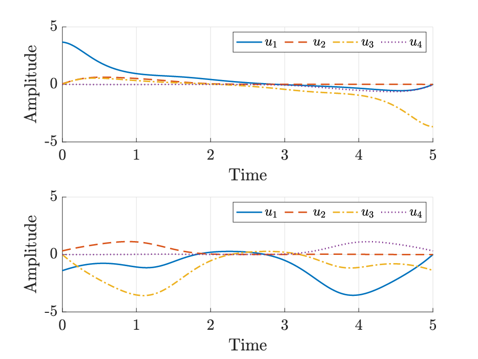
Figure 5: Optimal control input sequences obtained when the objectives are to minimize the control effort (Top) or prevent the system from populating |2⟩\ket{2} (Bottom).
Refer to caption
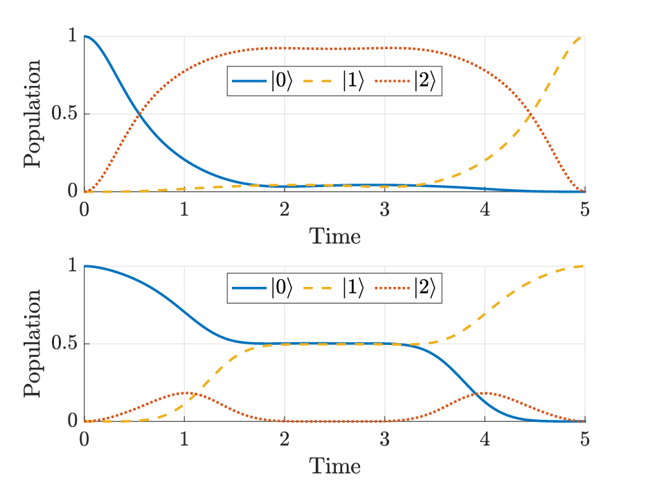
Figure 6: Population dynamics obtained under the optimal control law that minimizes the control effort (Top) or prevents the system from populating |2⟩\ket{2} (Bottom).

Minimize Control Effort
First, we consider a incremental cost that only penalizes the control effort, i.e.

ℓ⁡(|ψ⟩,u,t)=12​uT​ℛ​(t)​u,\ell(\ket{\psi}\!,u,t\big)=\tfrac{1}{2}u^{T}\mathcal{R}(t)\,u, (57)

where

ℛ⁡(t)=0.1​[0.010000r⁡(t)+1.100000.010000−r⁡(t)+1.1],\mathcal{R}(t)=0.1\begin{bmatrix}0.01&0&0&0\\ 0&r(t)+1.1&0&0\\ 0&0&0.01&0\\ 0&0&0&-r(t)+1.1\end{bmatrix},

and r⁡(t)=tanh⁡(2​t−T)r(t)=\tanh(2t-T). Figure 5a shows the optimal control input u⁡(t)u(t) and Figure 6a shows the population evolves in time. Although almost all population goes to the target state at the end (t=5t=5), we can clearly observe that there is over 90%90\% of the population going through the state |2⟩\ket{2} for t∈(1,4)t\in(1,4). This behavior may be undesirable for some applications. The solver took 1111 iterations to obtain the solution.

Minimize Undesirable Population
To avoid populating the |2⟩\ket{2} state as much as possible, consider the incremental cost

ℓ⁡(|ψ⟩,u,t)=12​uT​ℛ​(t)​u+12​𝔮​⟨ψ|​Γ¯2​|ψ⟩,\ell(\ket{\psi}\!,u,t\big)=\tfrac{1}{2}u^{T}\mathcal{R}(t)\,u+\tfrac{1}{2}\mathfrak{q}\bra{\psi}\overline{\Gamma}_{2}\ket{\psi}, (58)

where ℛ⁡(t)\mathcal{R}(t) is the same as (57) and 𝔮=0.1\mathfrak{q}=0.1, Γ¯2=|2⟩⟨2|\overline{\Gamma}_{2}=\left|{2}\middle\rangle\!\middle\langle{2}\right| define a new cost that penalizes |2⟩\ket{2}.

Figures 5b and 6b show the optimal control input u⁡(t)u(t) and the population |ψ⁡(t)⟩\ket{\psi(t)}, respectively. In this case, the system successfully transitions from |0⟩\ket{0} to |1⟩\ket{1} while maintaining a limited (<20%<20\%) presence in the undesirable population |2⟩\ket{2}. The solver took 1919 iterations to obtain the solution.

V.3 X-Gate for a Fluxonium Qubit

We now show how to design a Pauli-X gate for a fluxonium qubit using Q-PRONTO. The Hamiltonian of the fluxonium qubit Manucharyan et al. 2009 is given by

H0=−4EC∂ϕ2−EJcos(ϕ−φext)+12ELϕ2,H_{0}=-4E_{C}\partial^{2}_{\phi}-E_{J}\cos{(\phi-\varphi_{\text{ext}}})+\frac{1}{2}E_{L}\phi^{2}, (59)

where ECE_{C} is the charging energy, EJE_{J} is the Josephson energy, ELE_{L} is the inductive energy, and φext\varphi_{\text{ext}} is the external flux in dimensionless form. Consider a truncated 3-level fluxonium qubit, whose Hamiltonian can be written as

i​ℏ​|ψ˙⟩=([E0000E1000E2]+u​[0Ω01Ω02Ω010Ω12Ω02Ω120])​|ψ⟩,\mathrm{i}\hbar\ket{\dot{\psi}}=\left(\!\begin{bmatrix}E_{0}&0&0\\ 0&E_{1}&0\\ 0&0&E_{2}\end{bmatrix}\!+\!u\begin{bmatrix}0&\Omega_{01}&\Omega_{02}\\ \Omega_{01}&0&\Omega_{12}\\ \Omega_{02}&\Omega_{12}&0\end{bmatrix}\!\right)\!\!\ket{\psi}, (60)

where E0=0E_{0}=0, E1=1​GHzE_{1}=1~\text{GHz}, E2=5​GHzE_{2}=5~\text{GHz} is the corresponding energy levels for the eigenstates |0⟩\ket{0}, |1⟩\ket{1} and |2⟩\ket{2}; Ω01=0.1\Omega_{01}=0.1, Ω12=0.5\Omega_{12}=0.5, Ω02=0.3\Omega_{02}=0.3 is the effort to transfer between eigenstates. Since |0⟩\ket{0} and |1⟩\ket{1} are the logical states for this qubit, we wish to design a Pauli X-gate: an optimal control input u⁡(t)u(t) so that it steers |0⟩\ket{0} to |1⟩\ket{1}, while simultaneously steering |1⟩\ket{1} to |0⟩\ket{0}. The optimal control problem can then be written as

min\displaystyle\displaystyle\min~~ ‖ψ0​(T)−|1⟩‖2+‖ψ1​(T)−|0⟩‖2+∫0Tl⁡(|ψ⟩,u,t)​𝑑t\displaystyle\|\psi_{0}(T)\!-\!\ket{1}\|^{2}+\|\psi_{1}(T)\!-\!\ket{0}\|^{2}+\int^{T}_{0}\!\!\!l(\ket{\psi},u,t)dt
s.t.   |ψ0˙⟩=H⁡(u)​|ψ0⟩,|ψ0​(0)⟩=|0⟩,\displaystyle\ket{\dot{\psi_{0}}}=H(u)\ket{\psi_{0}},\qquad\ket{\psi_{0}(0)}=\ket{0}, (61b)
|ψ1˙⟩=H⁡(u)​|ψ1⟩,|ψ1​(0)⟩=|1⟩.\displaystyle\ket{\dot{\psi_{1}}}=H(u)\ket{\psi_{1}},\qquad\ket{\psi_{1}(0)}=\ket{1}.

We propose two different incremental costs, but for both cases, we set the time horizon T=10T=10 ns and use the same initial guess pulse

u0​(t)=πT​e−(t−T/2)2T2​cos⁡2​π​t.u_{0}(t)=\frac{\pi}{T}e^{\frac{-(t-T/2)^{2}}{T^{2}}}\cos{2\pi t}.

The exit condition is tol=10−4\texttt{tol}=10^{-4}.

Refer to caption
Figure 7: Optimal control input sequences obtained when the objectives are to minimize the control effort (Top) or to prevent the system from populating |2⟩\ket{2} (Bottom).

Minimize Control Effort
First, we consider a incremental cost that only penalizes the control effort, i.e.

ℓ⁡(|ψ⟩,u,t)=12​uT​u.\ell(\ket{\psi}\!,u,t\big)=\tfrac{1}{2}u^{T}u. (62)

Figure 7a shows the optimal control input u⁡(t)u(t) and Figures 8a–9a show how the two basis vectors |ψ0⟩\ket{\psi_{0}} and |ψ1⟩\ket{\psi_{1}} evolve over time. Although the quantum gate fidelity Pedersen et al. 2007

ℱ=(d+|Tr⁡(U​Utarg†)|2)/(d2+d)\mathcal{F}=(d+|\mathrm{Tr}(UU_{\text{targ}}^{\dagger})|^{2})/(d^{2}+d)

is greater than 99.9%99.9\%, we can clearly observe that over 50%50\% of the population transitions through the state |2⟩\ket{2} during the process. The solver took 1010 iterations to obtain the solution.

Refer to caption
Figure 8: Population dynamics of the |0⟩→|1⟩\ket{0}\!\to\!\ket{1} transition under the optimal control law that minimizes the control effort (Top) or prevents the system from populating |2⟩\ket{2} (Bottom). The transient peak of |2⟩\ket{2} is reduced from .58.58 to .03.03.
Refer to caption
Figure 9: Population dynamics of the |1⟩→|0⟩\ket{1}\!\to\!\ket{0} transition under the optimal control law that minimizes the control effort (Top) or prevents the system from populating |2⟩\ket{2} (Bottom). The behavior roughly mirrors the |0⟩→|1⟩\ket{0}\!\to\!\ket{1} transition.

Minimize Undesirable Population
To avoid populating the |2⟩\ket{2} state as much as possible, consider the incremental cost

ℓ⁡(|ψ⟩,u,t)=12​uT​u+12​𝔮​(⟨ψ0|​Γ¯2​|ψ0⟩+⟨ψ1|​Γ¯2​|ψ1⟩),\ell(\ket{\psi}\!,u,t\big)=\tfrac{1}{2}u^{T}u+\tfrac{1}{2}\mathfrak{q}(\bra{\psi_{0}}\overline{\Gamma}_{2}\ket{\psi_{0}}+\bra{\psi_{1}}\overline{\Gamma}_{2}\ket{\psi_{1}}), (63)

where 𝔮=0.3\mathfrak{q}=0.3 and Γ¯2=|2⟩⟨2|\overline{\Gamma}_{2}=\left|{2}\middle\rangle\!\middle\langle{2}\right| penalize |2⟩\ket{2}.

Figures 7b and 8b–9b show the optimal control input u⁡(t)u(t) and the basis vector dynamics |ψ0​(t)⟩\ket{\psi_{0}(t)}, |ψ1​(t)⟩\ket{\psi_{1}(t)}, respectively. In this case, the gate fidelity remains greater than 99.9%99.9\% while maintaining a limited (<3%<3\%) presence in the |2⟩\ket{2} population during the whole process. However, the control amplitude becomes much higher, with the maximum amplitude reaching 2​GHz2\text{GHz}. Note that the tradeoff between maximum input amplitude and maximum |2⟩\ket{2} population can be explored by tuning 𝔮≥0\mathfrak{q}\geq 0. The solver took 44 iterations to obtain the solution.

VI Conclusions

This paper augments the Quantum Projection Operator-based Newton method for Trajectory Optimization (Q-PRONTO) with a quantum-specific regulator designed to stabilize the system trajectories to the spherical manifold. The method is not only faster due to the presence of the regulator, but may also converge to better local minima compared to the unregulated case.

Additionally, the paper introduces new capabilities to Q-PRONTO, such as the ability to incorporate time-varying cost functions and to avoid undesirable populations during the transient. Future research directions include the design of unitary gates, control of open quantum systems, and in-depth comparisons with existing optimization methods. Q-PRONTO is set to be released as an open source Julia package over the next year.

Acknowledgements The authors would like to thank Joshua Combes, András Gyenis, Murray Holland, and Liang-Ying Chih for their valued collaboration and helpful insights. This work is supported by the NSF QII–TAQS award number 1936303.

References

  • Brif et al. (2010) C. Brif, R. Chakrabarti, and H. Rabitz, Control of quantum phenomena: past, present and future, New Journal of Physics 12, 075008 (2010).
  • Dong and Petersen (2010) D. Dong and I. R. Petersen, Quantum control theory and applications: a survey, IET control theory & applications 4, 2651 (2010).
  • Altafini and Ticozzi (2012) C. Altafini and F. Ticozzi, Modeling and control of quantum systems: An introduction, IEEE Transactions on Automatic Control 57, 1898 (2012).
  • Glaser et al. (2015) S. J. Glaser, U. Boscain, T. Calarco, C. P. Koch, W. Köckenberger, R. Kosloff, I. Kuprov, B. Luy, S. Schirmer, T. Schulte-Herbrüggen, et al., Training schrödinger’s cat: quantum optimal control, The European Physical Journal D 69, 1 (2015).
  • Khaneja et al. (2001) N. Khaneja, R. Brockett, and S. J. Glaser, Time optimal control in spin systems, Physical Review A 63, 032308 (2001).
  • Khaneja et al. (2005) N. Khaneja, T. Reiss, C. Kehlet, T. Schulte-Herbrüggen, and S. J. Glaser, Optimal control of coupled spin dynamics: design of nmr pulse sequences by gradient ascent algorithms, Journal of magnetic resonance 172, 296 (2005).
  • Sklarz and Tannor (2002) S. E. Sklarz and D. J. Tannor, Loading a bose-einstein condensate onto an optical lattice: An application of optimal control theory to the nonlinear schrödinger equation, Physical Review A 66, 053619 (2002).
  • Reich et al. (2012) D. M. Reich, M. Ndong, and C. P. Koch, Monotonically convergent optimization in quantum control using krotov’s method, The Journal of chemical physics 136, 104103 (2012).
  • de Fouquieres et al. (2011) P. de Fouquieres, S. G. Schirmer, S. J. Glaser, and I. Kuprov, Second order gradient ascent pulse engineering, Journal of Magnetic Resonance 212, 412 (2011).
  • Eitan et al. (2011) R. Eitan, M. Mundt, and D. J. Tannor, Optimal control with accelerated convergence: Combining the krotov and quasi-newton methods, Physical Review A 83, 053426 (2011).
  • Shao et al. (2022) J. Shao, J. Combes, J. Hauser, and M. M. Nicotra, Projection-operator-based newton method for the trajectory optimization of closed quantum systems, Physical Review A 105, 032605 (2022).
  • Hauser (2002) J. Hauser, A projection operator approach to the optimization of trajectory functionals, IFAC Proceedings Volumes 35, 377 (2002).
  • Hauser (2003) J. Hauser, On the computation of optimal state transfers with application to the control of quantum spin systems, in Proceedings of the 2003 American Control Conference, 2003., Vol. 3 (2003) pp. 2169–2174 vol.3.
  • Goerz et al. (2019) M. H. Goerz, D. Basilewitsch, F. Gago-Encinas, M. G. Krauss, K. P. Horn, D. M. Reich, and C. P. Koch, Krotov: A Python implementation of Krotov’s method for quantum optimal control, SciPost Phys. 7, 80 (2019).
  • Anderson and Moore (2007) B. D. O. Anderson and J. B. Moore, Optimal Control: Linear Quadratic Methods, Dover Books on Engineering (2007).
  • Shao et al. (2023) J. Shao, L.-Y. Chih, M. Naris, M. Holland, and M. M. Nicotra, Application of quantum optimal control to shaken lattice interferometry, in 2023 American Control Conference (ACC) (2023) pp. 4593–4598.
  • Nicotra et al. (2023) M. M. Nicotra, J. Shao, J. Combes, A. C. Theurkauf, P. Axelrad, L.-Y. Chih, M. Holland, A. A. Zozulya, C. K. LeDesma, K. Mehling, et al., Modeling and control of ultracold atoms trapped in an optical lattice: An example-driven tutorial on quantum control, IEEE Control Systems Magazine 43, 28 (2023).
  • Manucharyan et al. (2009) V. E. Manucharyan, J. Koch, L. I. Glazman, and M. H. Devoret, Fluxonium: Single cooper-pair circuit free of charge offsets, Science 326, 113 (2009).
  • Pedersen et al. (2007) L. H. Pedersen, N. M. Møller, and K. Mølmer, Fidelity of quantum operations, Physics Letters A 367, 47 (2007).

Appendix A Wavefunction to State Mapping

For the reader’s convenience, this section provides some background on how to use the bijective mapping (15) to seamlessly transition between the (1) and (14). For the purpose of this section, let a∈ℝn,b∈ℝna\in\mathbb{R}^{n},~b\in\mathbb{R}^{n} be two real column vectors and define

x=[ab],|ψ⟩=a+i​bx=\begin{bmatrix}a\\ b\end{bmatrix},\qquad\ket{\psi}=a+\mathrm{i}b (64)

so that (15) is satisfied. Then, given the real matrices A∈ℝn×n,B∈ℝn×nA\in\mathbb{R}^{n\times n},~B\in\mathbb{R}^{n\times n} we note that

|ψ′⟩=(A+i​B)​|ψ⟩=(A​a−B​b)+i⁡(A​b+B​a)\ket{\psi^{\prime}}=(A+\mathrm{i}B)\ket{\psi}=(Aa-Bb)+\mathrm{i}(Ab+Ba) (65)

satisfies the bijective mapping (15) for

x′=[A−BBA]​x=[A​a−B​bA​b+B​a].x^{\prime}=\begin{bmatrix}A&-B\\ B&~~A\end{bmatrix}x=\begin{bmatrix}Aa-Bb\\ Ab+Ba\end{bmatrix}. (66)

As such, the induced matrix mapping

M=[Re⁡(ℳ)−Im⁡(ℳ)Im⁡(ℳ)Re⁡(ℳ)],ℳ=[I​i​I]​MM=\begin{bmatrix}\mathrm{Re}(\mathcal{M})&-\mathrm{Im}(\mathcal{M})\\ \mathrm{Im}(\mathcal{M})&~~\mathrm{Re}(\mathcal{M})\end{bmatrix},\qquad\mathcal{M}=[\,I~~\mathrm{i}I\,]M (67)

ensures that the state vector x′=M​xx^{\prime}=Mx remains consistent with the wavefunction |ψ′⟩=ℳ​|ψ⟩\ket{\psi^{\prime}}=\mathcal{M}\ket{\psi}. Based on these considerations, we show the following.

A.1 Schrödinger Equation

The Schrödinger equation |ψ˙⟩=ℋ​|ψ⟩\ket{\dot{\psi}}=\mathcal{H}\ket{\psi} can be rewritten as x˙=H​x\dot{x}=Hx with

H=[0I−I0]​[Re⁡(ℋ)−Im⁡(ℋ)Im⁡(ℋ)Re⁡(ℋ)].H=\begin{bmatrix}~~0&I~\\ -I&0~\end{bmatrix}\begin{bmatrix}\mathrm{Re}(\mathcal{H})&-\mathrm{Im}(\mathcal{H})\\ \mathrm{Im}(\mathcal{H})&~~\mathrm{Re}(\mathcal{H})\end{bmatrix}. (68)

This can be shown by applying the induced matrix mapping (67) to the equation |ψ˙⟩=−i​ℋ​|ψ⟩\ket{\dot{\psi}}=-\mathrm{i}\mathcal{H}\ket{\psi}. Note that, if ℋ\mathcal{H} is Hermitian (i.e., ℋ†=ℋ\mathcal{H}^{\dagger}=\mathcal{H}), i​ℋ\mathrm{i}\mathcal{H} is skew-Hermitian, which makes HH skew-symmetric (i.e., HT=−HH^{T}=-H). This is sufficient to ensure that ‖x⁡(t)‖\|x(t)\| remains constant, since

dd​t​‖x‖2=x˙T​x+xT​x˙=xT​(HT+H)​x=0.\frac{d}{dt}\|x\|^{2}=\dot{x}^{T}x+x^{T}\dot{x}=x^{T}(H^{T}+H)x=0. (69)

A.2 Quadratic Costs

Although it is possible to find an equivalent mapping for any cost function, this paper only addresses quadratic cost functions

c=⟨ψ|​𝒬​|ψ⟩,c=\bra{\psi}\mathcal{Q}\ket{\psi}, (70)

where 𝒬=A+i​B\mathcal{Q}=A+\mathrm{i}B is poisitive semi-definite and Hermitian (i.e., AA symmetric and BB skew-symmetric). Using (64), it is possible to show that

c=(aT−i​bT)​(A+i​B)​(a+i​b)=aT​A​a+bT​A​b.c=(a^{T}-\mathrm{i}b^{T})(A+\mathrm{i}B)(a+\mathrm{i}b)=a^{T}\!Aa+b^{T}\!Ab. (71)

Since the same output can also be obtained by computing

c=xT​[A00A]​x,c=x^{T}\begin{bmatrix}A&0\\ 0&A\end{bmatrix}x, (72)

it is possible to define the induced quadratic cost matrix

Q=[Re⁡(𝒬)00Re⁡(𝒬)].Q=\begin{bmatrix}\mathrm{Re}(\mathcal{Q})&0\\ 0&\mathrm{Re}(\mathcal{Q})\end{bmatrix}. (73)

For example, given 𝒬=|ψ⟩⟨ψ|\mathcal{Q}=\left|{\psi}\middle\rangle\!\middle\langle{\psi}\right|, we obtain

𝒬=(a+i​b)​(aT−i​bT)=(a​aT+b​bT)+i⁡(b​aT−a​bT),\mathcal{Q}=(a+\mathrm{i}b)(a^{T}-\mathrm{i}b^{T})=(aa^{T}+bb^{T})+\mathrm{i}(ba^{T}-ab^{T}),

which entails

Q=[a​aT+b​bT00a​aT+b​bT].Q=\begin{bmatrix}aa^{T}+bb^{T}&0\\ 0&aa^{T}+bb^{T}\end{bmatrix}. (74)

Appendix B Q-PRONTO Algorithm

Algorithm 1   Q-PRONTO
1: Input
2: Initial Guess
3: η0=(α0​(t),μ0​(t))\eta_{0}=(\alpha_{0}(t),\mu_{0}(t))
4: Initialization
5: Pre-Projection
6: [A0​(t),B0​(t)]←(23)[A_{0}(t),B_{0}(t)]\leftarrow\eqref{eq:LinDyn}, with (x⁡(t),u⁡(t))=η0(x(t),u(t))=\eta_{0}
7: [Qr​(t),Rr​(t),Πr]←(48)[Q_{r}(t),R_{r}(t),\Pi_{r}]\leftarrow\eqref{eq:cost_arbitrary}
8: Compute Kr​(t)K_{r}(t) ⊳\triangleright B.i.t. (43)
9: Initial Trajectory and Starting Cost
10: ξk←𝒫⁡(η0)\xi_{k}\leftarrow\mathcal{P}(\eta_{0})⊳\triangleright F.i.t. (21)
11: gk←(17)g_{k}\leftarrow\eqref{eq:cost}
12: Main Loop
13: D​g=−10​tolDg=-10\,\textrm{tol}
14: while −D​g≥tol-Dg\geq\textrm{tol} do
15: Compute Tangent Space and Linear Terms
16:   [Ak​(t),Bk​(t)]←(23)[A_{k}(t),B_{k}(t)]\leftarrow\eqref{eq:LinDyn}
17:   [qk​(t),rk​(t),πk]←(32)[q_{k}(t),r_{k}(t),\pi_{k}]\leftarrow\eqref{eq:LinCost}
18: Compute Regulator and Adjoint State
19:   [Qr​(t),Rr​(t),Πr]←(48)[Q_{r}(t),R_{r}(t),\Pi_{r}]\leftarrow\eqref{eq:cost_arbitrary}
20:   Compute Kr​(t)K_{r}(t) ⊳\triangleright B.i.t. (43)
21:   Compute χk​(t)\chi_{k}(t) ⊳\triangleright B.i.t. (38)
22: Perform (quasi-)Newton Step
23:   try
24:      [Qk​(t),Sk​(t),Rk​(t),Πk]←[Q_{k}(t),S_{k}(t),R_{k}(t),\Pi_{k}]\leftarrow(39)
25:      Compute [Ko​(t),vo​(t)][K_{o}(t),v_{o}(t)] ⊳\triangleright B.i.t. (40)
26:   catch (40) failed to converge do
27:      [Qk​(t),Sk​(t),Rk​(t),Πk]←[Q_{k}(t),S_{k}(t),R_{k}(t),\Pi_{k}]\leftarrow(33)
28:      Compute [Ko​(t),vo​(t)][K_{o}(t),v_{o}(t)] ⊳\triangleright B.i.t. (40)
29:   end try
30:   Compute ζk​(t)\zeta_{k}(t)⊳\triangleright F.i.t. (41)
31: Compute Cost Gradient
32:   D​gk←πk​zk​(T)+∫0Tqk​(t)​zk​(t)+rk​(t)​νk​(t)​𝑑tDg_{k}\leftarrow\pi_{k}z_{k}(T)+\int_{0}^{T}q_{k}(t)z_{k}(t)+r_{k}(t)\nu_{k}(t)dt
33: Armijo Step
34:   σ←min⁡( 1, 0.6​‖x0‖/max⁡(‖zk​(t)‖))\sigma\leftarrow\min(\,1\,,\,0.6\|x_{0}\|/\max(\|z_{k}(t)\|)\,)
35:   ξk+1←𝒫⁡(ξk​(t)+σ​ζk​(t))\xi_{k+1}\leftarrow\mathcal{P}(\xi_{k}(t)+\sigma\zeta_{k}(t))⊳\triangleright F.i.t. (21)
36:   gk+1←(17)g_{k+1}\leftarrow\eqref{eq:cost}
37:   while gk+1>gk−0.4​D​gkg_{k+1}>g_{k}-0.4\,Dg_{k} do
38:    σ←0.7​σ\sigma\leftarrow 0.7\,\sigma
39:    ξk+1←𝒫⁡(ξk​(t)+σ​ζk​(t))\xi_{k+1}\leftarrow\mathcal{P}(\xi_{k}(t)+\sigma\zeta_{k}(t))⊳\triangleright F.i.t. (21)
40:    gk+1←(17)g_{k+1}\leftarrow\eqref{eq:cost}
41:   end while
42: Proceed to Next Iteration
43:   ξk←ξk+1\xi_{k}\leftarrow\xi_{k+1}
44:   gk←gk+1g_{k}\leftarrow g_{k+1}
45: end while
46: Output
47: Solution
48: return [x⁡(t),u⁡(t)]=ξk[x(t),u(t)]=\xi_{k}
49:  
50: F.i.t. = Integrate forward in time
51: B.i.t. = Integrate backward in time