Ubiquitous nematic Dirac semimetal emerging from interacting quadratic band touching system
Abstract
Quadratic band touching (QBT) points are widely observed in 2D and 3D materials, including bilayer graphene and Luttinger semimetals, and attract significant attention from theory to experiment. However, even in its simplest form, the 2D checkerboard lattice QBT model, the phase diagram characterized by temperature and interaction strength still remains unknown beyond the weak-coupling regime. Intense debates persist regarding the existence of various interaction-driven insulating states in this system Sun et al. 2009; Uebelacker and Honerkamp 2011; Wu et al. 2016; Sur et al. 2018; Zeng et al. 2018; Lu et al. 2022; Ji et al. 2022. To address these uncertainties, we employ thermal tensor network simulations, specifically exponential tensor renormalization group and tangent space tensor renormalization group Chen et al. 2018; Li et al. 2023, along with density matrix renormalization group calculations to provide a comprehensive finite-temperature phase diagram for this model and shed light on previous ambiguities. Notably, our findings reveal the emergence of a robust bond-nematic Dirac semimetal phase with distinct thermodynamic properties that set it part from the nematic insulating state and other symmetry broken states. This previously overlooked feature is found to be ubiquitous in interacting QBT systems. We also discuss the implications of these results for experimental systems such as bilayer graphene and iridate compounds.
Introduction.— Quadratic band touching (QBT) points are widely observed in materials. In the 2D realm, bilayer graphene serves as a representative example Yan et al. 2011; Lang et al. 2012; Pujari et al. 2016; Ray et al. 2018; Ray and Janssen 2021, while in 3D, materials like -Sn, HgTe, and pyrochlore iridates Ir2O7 ( Pr, Nd) exhibit Luttinger semimetal behavior Luttinger 1956; Moon et al. 2013; Herbut and Janssen 2014; Cheng et al. 2017; Wang et al. 2020; Kondo et al. 2015; Boettcher and Herbut 2017; Janssen and Herbut 2017; Kharitonov et al. 2022. Investigating the effects of interactions on QBTs is both fundamentally significant and experimentally relevant. For instance, understanding how QBTs transform into symmetry-breaking phases in bilayer graphene under the influence of trigonal warping and Coulomb interactions, or how Luttinger semimetals can evolve into Dirac, line-nodal, or Weyl semimetals, and even non-Fermi-liquid states in the presence of strain, bulk-inversion asymmetry, and Coulomb interactions, remains an active area of intense theoretical and experimental investigations Yan et al. 2011; Lang et al. 2012; Pujari et al. 2016; Ray et al. 2018; Ray and Janssen 2021; Moon et al. 2013; Herbut and Janssen 2014; Cheng et al. 2017; Wang et al. 2020; Kondo et al. 2015; Boettcher and Herbut 2017; Janssen and Herbut 2017; Kharitonov et al. 2022.

The 2D checkerboard lattice model with symmetry serves as the simplest platform to investigate the effects of interactions on QBTs. Previous studies have revealed that a quantum anomalous Hall (QAH) state with spontaneously broken time-reversal symmetry (TRS) Thouless et al. 1982; von Klitzing et al. 2020; Haldane 1988; Chang et al. 2013; Deng et al. 2020; Stepanov et al. 2021; Haldane 2004; Nagaosa et al. 2010; Xiao et al. 2010; Raghu et al. 2008; Chen et al. 2021a; Liu and Dai 2021; Lin et al. 2022a; Pan et al. 2023; Zhang et al. 2023; Lin et al. 2022b; Huang et al. 2023 emerges in the weak-coupling regime Sun et al. 2009; Uebelacker and Honerkamp 2011; Wu et al. 2016; Sur et al. 2018; Zeng et al. 2018; Lu et al. 2022. Proposals have also been put forth to realize QBT and interaction-driven QAH states in real materials, which include the four-band checkerboard lattice system based on monolayer CrCl2(pyrazine)2 Ji et al. 2022, as well as the symmetric Kagome metals Nishimoto et al. 2010; Wen et al. 2010; Zhu et al. 2016; Hui et al. 2018; Sankar et al. 2023; Ren et al. 2018.
Beyond the weak-couling regime, the QAH phase is anticipated to give way to other competing phases, such as the symmetric site-nematic insulator SNI Sun et al. 2009. However, due to the strong coupling nature of these phases, a complete phase diagram remains a subject of debate, with conflicting results Sun et al. 2009; Uebelacker and Honerkamp 2011; Wu et al. 2016; Sur et al. 2018; Zeng et al. 2018; Lu et al. 2022; Ji et al. 2022. Exact diagonalization (ED) and density matrix renormalization group (DMRG) simulations suggest that there is no co-existing region between the QAH and SNI states Wu et al. 2016. Instead, a symmetry-breaking bond-nematic Dirac semimetal (BNDS) phase emerges as an intermediate phase, where the QBT splits into two Dirac cones Zeng et al. 2018. Notably, the BNDS and SNI were identified as distinct thermodynamic phases with different order parameters Zeng et al. 2018.
The transitions between QAH, BNDS, and SNI phases are found to be first-order, different from the interaction-driven phase transitions in Bernal stacking graphene Lang et al. 2012; Pujari et al. 2016; Ray et al. 2018; Ray and Janssen 2021. And the previous studies Sun et al. 2009; Uebelacker and Honerkamp 2011; Wu et al. 2016; Zeng et al. 2018 considered only nearest-neighbor (NN) interactions without next-nearest-neighbor (NNN) interactions, which are crucial for understanding the transition to other interaction-driven states such as the stripe-like charge density wave insulator (Stripe). Furthermore, the relationship between the BNDS and SNI phases has not been adequately addressed, and we demonstrate that they break exactly the same symmetry.
By incorporating NNN interactions into the system, Ref. Sur et al. 2018 observed a direct transition from QAH or Stripe to the SNI phase, omitting the BNDS phase. In a Hartree-Fock study of a doubled four-band checkerboard lattice Ji et al. 2022, the BNDS phase was not reported. Instead, they discovered a Dirac semimetal phase with site-nematic order between the site-nematic insulator and the QBT semimetal. These discrepancies highlight the ongoing challenges in achieving a consensus on the ground state phase diagram of the checkerboard lattice QBT system. Furthermore, the finite-temperature phase diagram, especially the distinct behavior from emergent Dirac cones of the interaction-driven BNDS phase, remains completely unexplored.
In this Letter, by employing the exponential and tangent space tensor renormalization groups (XTRG and tanTRG) Chen et al. 2018; Li et al. 2023 and DMRG calculations, we unveil a comprehensive phase diagram based on thermodynamic characteristics. One key finding is the ubiquitous presence of the BNDS phase, which separates not only the QAH and SNI phases, but also the Stripe and SNI phases. We clarify the equivalence of SNI and BNDS in terms of symmetry and reveal their distinct measurable properties, especially in their different thermodynamic properties. We foresee this overlooked interaction-driven BNDS with emergent Lorentz symmetry and unique thermodynamic properties could be a universal feature in interacting QBT systems, extending beyond the checkerboard lattice, with potential realizations in bilayer graphene Lang et al. 2012; Pujari et al. 2016; Ray et al. 2018; Ray and Janssen 2021, -Sn, HgTe and iridate compounds Luttinger 1956; Moon et al. 2013; Herbut and Janssen 2014; Cheng et al. 2017; Wang et al. 2020; Kondo et al. 2015; Boettcher and Herbut 2017; Janssen and Herbut 2017; Kharitonov et al. 2022.

Model, Method and Ground-State Phase Diagram.— We examine a spinless fermion model in a checkerboard lattice,
| (1) | |||||
with , being the sublattice index, and , as shown in Fig. 1(a). We fix and and consider both the repulsive NN and NNN density-density interactions.
We mainly employ the XTRG and tanTRG method Chen et al. 2018; Li et al. 2019; Li et al. 2023 for finite-temperature simulationsChen et al. 2019; Li et al. 2019; Li et al. 2020; Chen et al. 2021b; Lin et al. 2022a; Qu et al. 2022 with YC geometry and we retain up to bond states, rendering the truncation errors down to the low- regime. We also perform YC DMRG simulations, with up to bond states and maximal truncation errors .

Here we set and systematically vary to demonstrate the existence of the BNDS phase between the QAH and SNI states. Additional numerical evidence supporting the presence of BNDS phases for different can be found in the Supplemental Materials (SM) sup. Furthermore, we investigate the large-interaction regime by fixing and varying , revealing the occurrence of the BNDS phase between the Stripe and SNI phases. The BNDS state is unambiously characterized from both the low- power law behaviour of specific heat (), and the changes of conformal central charge and the single-particle excitation gap via flux insertion. Consequently, we construct a comprehensive ground-state phase diagram, as illustrated in Fig. 1(b). Additionally, through comparing the symmetry of the two nematic states, BNDS and SNI, we find both states break exactly the same symmetry. In other words, akin to the gas-liquid and/or Lifshitz transitions, the first-order phase boundary between them does not involve a change in symmetry.
it is possible for the establishment of an adiabatic pathway between these two states through exploring a higher-dimensional phase space. Regarding the bond- and site-nematic order parameters, without fine-tuning, both of these order parameters remain nonzero in both the BNDS and SNI phases, reflecting their identical symmetry. This finding contrasts with the numerical results obtained from finite-size extrapolation as reported in previous work Zeng et al. 2018. phase diagram and the thermodynamic characteristics.— To identify different phases in the phase diagram, we utilize several measurements: QAH structure factor , where the summation is over NN bonds in the bulk with being the total number of bonds and charactering the orientation of the current ; bond nematic order parameter , which measures the difference in NNN hopping amplitudes along the vertical () and horizontal () directions; site nematic order parameter , which quantifies the difference of electron density at ‘A’ and ‘B’ sublattices; structure factor for the Stripe phase , where represents the Stripe pattern shown in Fig. 1(d); the specific heat , where is the energy density.
In Fig. 2(a-d), we present various order parameters and structure factors respectively. At , when is small (Fig. 2(a)), the ground state is a SNI, and the order parameter , as well as the transition temperature, reduces as increases. In Fig. 2(b), an intermediate BNDS phase between QAH and SNI is clearly observed. This phase exhibits a strong bond nematic order Notably, the site nematic order is also present in the BNDS region and becomes stronger as decreases, ultimately exhibiting a significant jump across the phase boundary to the SNI phase. Furthermore, a sharp change in the QAH (Fig.2(c)) and Stripe (Fig.2(d)) structure factors near the phase boundary indicates a first-order transition between these two phases. The specific heat shown in Fig. 2(e) also supports the identification of these phases with distinct characteristics.
To analyze the detailed thermodynamic transitions and features, we present four cuts of the 2D phase diagrams in Fig. 3. These cuts are taken along the temperature axis at fixed interactions, corresponding to four different ground states. At high temperatures (much larger than the band width), the specific heat exhibits a scaling behavior of for all cases. A crossover temperature can be identified where deviates from the scaling, below which, displays two peaks or shoulders. The lower-temperature one, marks the transition to the low- ground state, which agrees with the order parameters / structure factors versus temperature , while the higher-temperature peak/shoulder is a thermodynamic characteristic of the electron band structure. With the latest tanTRG method, we are capable of fitting the low- behavior of , which has the exponential activation of in QAH, SNT and Stripe phases. While more importantly, we can see the behavior of low- in BNDS phase, which is the expected behavior of 2D Dirac cones and further supports the BNDS phase is actually a Dirac semimetal, emerging from interaction-driven QBT systems.
We note that for the thermodynamics of QAH state, at , both its transition temperature and the amplitude of the loop current exhibit little dependence on , as illustrated in Fig. 2(c) and SM sup. In contrast, when is set to zero, the transition temperature and the amplitude of the loop current of the QAH state exhibit a strong dependence on . As increases, both these two quantities increase before saturating at certain constant values. Besides, we add the DMRG results of QAH order parameters to SM sup for more evidence of QAH state, which agrees with the finite-temperature phase diagram.

More importantly, with larger interactions, the QAH phase disappears, but the BNDS always survives as an intermediate phase between SNI and Stripe, in direct contrast to the predictions from all existing studies. The color figures in Fig.4(a-c), clearly depict the Stripe-BNDS-SNI transition, with fixed and varying . To further verify the presence of the intermediate BNDS phase, we perform DMRG simulations within the BNDS phase and extract the conformal central charge from the entanglement entropy. By fitting the entanglement entropy as a function of the cylinder length to the universal scaling function , we obtain a central charge with (which is still far from convergence), as shown in Fig. 4(d) and SMsup, which directly supports the existence of Dirac cones with emergent Lorentz symmetry in the BNDS phase. To further check the location of Dirac cones, we implement the twisted boundary conditions in the direction by inserting the flux , , for all hopping terms across the boundary. For the same parameters in BNDS phase, with and , we fit the central charge with certain flux , compared with that of no flux, and also measure the single-particle gap by extrapolating the ground-state energy at half-filling sector and lowest energy in the single-particle-excited sector (details in SMsup). As shown in Fig.4(e), It is clear that the positions of Dirac cone are close to with a minute shift approximated (as denoted by the minimal of the single-particle gap, where the fitted central charge also saturates at its peak value), which is consistent with the meanfield analysis in the SM sup, and in this sense, the YC6 cylinder geometry is already close to be able to host the Dirac cones in the BNDS phase and our evidence of the Dirac cones are robust.
Furthermore, it is noteworthy that the strength of the NNN bond order in different regions of the BNDS phase remains almost constant around 0.1, as depicted in Fig. 5(c). Combining simulations at different and , the phase diagram shown in Fig. 1(b) indicate that this BNDS arises universally as an intermediate phase between SNI and all other grounds states in the phase space.
Mechanism of phase transition and nematic phases.— We further perform mean-field analysis to better understand the transitions and the bond (site) nematic phases. For the BNDS, we change the NNN hopping in Eq. (1) with positive ; for the SNI, we add sublattice chemical potential to Eq. (1). At the quadratic level, a finite value of both and will split the QBT at () into two Dirac cones. From the perspective of symmetries, the QAH state breaks the TRS, while the BNDS and SNI states break the same lattice rotation symmetry into the same symmetry. In fact, our mean-field calculation (c.f. SM sup) shows, the site (bond) nematic term will also induce bond (site) order, which is consistent with our numerical results and clarifies the confusion in previous work Zeng et al. 2018, that the two nematic orders should be the same.

The difference between SNI and BNDS is not in symmetry but in their physical properties including, 1) with sufficiently strong site-nematic order , the two Dirac cones will merge and gap out as shown in Fig. 5(a), whereas the bond-nematic term cannot gap out the Dirac cone; 2) right after the gap-open point, the sign structure of the NNN hopping amplitudes changes and the signs within the same sublattice become the same as shown in Fig. 5(b). We thus utilize such a feature to distinguish the SNI with BNDS phase. Such as in the - phase diagram Fig. 5(d), the sign structure of NNN hoppings clearly gives the SNI-BNDS boundary.
In our mean-field analysis, with the increase of , the two Dirac cones gradually merge into each other at the periodic boundary, and gap out the system, corresponding to the SNI observed. In reality, between the BNDS and SNI phases is an abrupt first-order transition, in that, although the two splited Dirac cones move away from the (,) point, they cannot gradually merge into each other in BNDS states but suddenly jump to SNI state with much larger around the first order transition, and the system is gapped out. Since there is no symmetry difference, the BNDS-SNI transition is similar to the liquid-gas transition, and one can in principle turn the first-order phase transition to an adiabatic crossover or a critical point through paths in higher-dimensional parameter space.
Discussions.—In conlusion, we find the interaction-driven BNDS ubiquitously exist beween SNI and the other interaction-driven insulating states in the checkerboard lattice QBT system, and we provide the complete ground state and finite-temperature phase diagram with repulsive interactions, which solves the previous debates in this system Sun et al. 2009; Uebelacker and Honerkamp 2011; Wu et al. 2016; Sur et al. 2018; Zeng et al. 2018; Lu et al. 2022; Ji et al. 2022. We find the transition between BNDS and SNI in the phase diagram is similar to the liquid-gas transition and provide the numerical results of the thermodynamic characteristics, in that the BNDS state is characterized by of emergent Dirac cones from interacting QBT systems, distinctively different from the exponential form in other phases. The interaction-driven BNDS, with emergent Lorentz symmetry and unique thermodynamic properties, can stimulate deeper understanding of the QBT systems and provide a new alternative interaction-driven Dirac semimetal in materials such as Kagome metals Nishimoto et al. 2010; Wen et al. 2010; Zhu et al. 2016; Hui et al. 2018; Ren et al. 2018; Sankar et al. 2023, bilayer graphene Lang et al. 2012; Pujari et al. 2016; Ray et al. 2018; Ray and Janssen 2021 and the -Sn, HgTe and iridate compound Ir2O7 ( Pr, Nd) Wang et al. 2020; Kondo et al. 2015; Boettcher and Herbut 2017; Janssen and Herbut 2017.
Acknowledgements.
Acknowledgments — We thank Wei Li and Michael Scherer for discussions, and we in particular thank Lukas Janssen for the enlightening introduction of Luttinger semimetals and discussion on the interaction effect on QBT. HYL thank Shou-Shu Gong for helpful discussions. HYL, BBC and ZYM acknowledge the support from the Research Grants Council (RGC) of Hong Kong SAR of China (Project Nos. 17301420, 17301721, AoE/P-701/20, 17309822, HKU C7037-22G), the ANR/RGC Joint Research Scheme sponsored by RGC of Hong Kong and French National Research Agency (Project No. A_HKU703/22), the K. C. Wong Education Foundation (Grant No. GJTD-2020-01). We thank HPC2021 system under the Information Technology Services and the Blackbody HPC system at the Department of Physics, University of Hong Kong for providing computational resources that have contributed to the research results in this paper.References
- Sun et al. (2009) K. Sun, H. Yao, E. Fradkin, and S. A. Kivelson, Phys. Rev. Lett. 103, 046811 (2009).
- Uebelacker and Honerkamp (2011) S. Uebelacker and C. Honerkamp, Phys. Rev. B 84, 205122 (2011).
- Wu et al. (2016) H.-Q. Wu, Y.-Y. He, C. Fang, Z. Y. Meng, and Z.-Y. Lu, Phys. Rev. Lett. 117, 066403 (2016).
- Sur et al. (2018) S. Sur, S.-S. Gong, K. Yang, and O. Vafek, Phys. Rev. B 98, 125144 (2018).
- Zeng et al. (2018) T.-S. Zeng, W. Zhu, and D. Sheng, npj Quantum Materials 3, 49 (2018).
- Lu et al. (2022) H. Lu, S. Sur, S.-S. Gong, and D. N. Sheng, Phys. Rev. B 106, 205105 (2022).
- Ji et al. (2022) X. Ji, J. Gao, C. Yue, Z. Wang, H. Wu, X. Dai, and H. Weng, Phys. Rev. B 106, 235103 (2022).
- Chen et al. (2018) B.-B. Chen, L. Chen, Z. Chen, W. Li, and A. Weichselbaum, Phys. Rev. X 8, 031082 (2018).
- Li et al. (2023) Q. Li, Y. Gao, Y.-Y. He, Y. Qi, B.-B. Chen, and W. Li, Phys. Rev. Lett. 130, 226502 (2023).
- Yan et al. (2011) K. Yan, H. Peng, Y. Zhou, H. Li, and Z. Liu, Nano Lett. 11, 1106 (2011).
- Lang et al. (2012) T. C. Lang, Z. Y. Meng, M. M. Scherer, S. Uebelacker, F. F. Assaad, A. Muramatsu, C. Honerkamp, and S. Wessel, Phys. Rev. Lett. 109, 126402 (2012).
- Pujari et al. (2016) S. Pujari, T. C. Lang, G. Murthy, and R. K. Kaul, Phys. Rev. Lett. 117, 086404 (2016).
- Ray et al. (2018) S. Ray, M. Vojta, and L. Janssen, Phys. Rev. B 98, 245128 (2018).
- Ray and Janssen (2021) S. Ray and L. Janssen, Phys. Rev. B 104, 045101 (2021).
- Luttinger (1956) J. M. Luttinger, Phys. Rev. 102, 1030 (1956).
- Moon et al. (2013) E.-G. Moon, C. Xu, Y. B. Kim, and L. Balents, Phys. Rev. Lett. 111, 206401 (2013).
- Herbut and Janssen (2014) I. F. Herbut and L. Janssen, Phys. Rev. Lett. 113, 106401 (2014).
- Cheng et al. (2017) B. Cheng, T. Ohtsuki, D. Chaudhuri, S. Nakatsuji, M. Lippmaa, and N. P. Armitage, Nature Communications 8, 2097 (2017).
- Wang et al. (2020) K. Wang, B. Xu, C. W. Rischau, N. Bachar, B. Michon, J. Teyssier, Y. Qiu, T. Ohtsuki, B. Cheng, N. P. Armitage, S. Nakatsuji, and D. v. d. Marel, Nature Physics 16, 1194 (2020).
- Kondo et al. (2015) T. Kondo, M. Nakayama, R. Chen, J. J. Ishikawa, E.-G. Moon, T. Yamamoto, Y. Ota, W. Malaeb, H. Kanai, Y. Nakashima, Y. Ishida, R. Yoshida, H. Yamamoto, M. Matsunami, S. Kimura, N. Inami, K. Ono, H. Kumigashira, S. Nakatsuji, L. Balents, and S. Shin, Nature Communications 6, 10042 (2015).
- Boettcher and Herbut (2017) I. Boettcher and I. F. Herbut, Phys. Rev. B 95, 075149 (2017).
- Janssen and Herbut (2017) L. Janssen and I. F. Herbut, Phys. Rev. B 95, 075101 (2017).
- Kharitonov et al. (2022) M. Kharitonov, J.-B. Mayer, and E. M. Hankiewicz, arXiv e-prints , arXiv:2212.00902 (2022), arXiv:2212.00902 [cond-mat.mes-hall] .
- Thouless et al. (1982) D. J. Thouless, M. Kohmoto, M. P. Nightingale, and M. den Nijs, Phys. Rev. Lett. 49, 405 (1982).
- von Klitzing et al. (2020) K. von Klitzing, T. Chakraborty, P. Kim, V. Madhavan, X. Dai, J. McIver, Y. Tokura, L. Savary, D. Smirnova, A. M. Rey, C. Felser, J. Gooth, and X. Qi, Nature Reviews Physics 2, 397 (2020).
- Haldane (1988) F. D. M. Haldane, Phys. Rev. Lett. 61, 2015 (1988).
- Chang et al. (2013) C.-Z. Chang, J. Zhang, X. Feng, J. Shen, Z. Zhang, M. Guo, K. Li, Y. Ou, P. Wei, L.-L. Wang, Z.-Q. Ji, Y. Feng, S. Ji, X. Chen, J. Jia, X. Dai, Z. Fang, S.-C. Zhang, K. He, Y. Wang, L. Lu, X.-C. Ma, and Q.-K. Xue, Science 340, 167 (2013).
- Deng et al. (2020) Y. Deng, Y. Yu, M. Z. Shi, Z. Guo, Z. Xu, J. Wang, X. H. Chen, and Y. Zhang, Science 367, 895 (2020).
- Stepanov et al. (2021) P. Stepanov, M. Xie, T. Taniguchi, K. Watanabe, X. Lu, A. H. MacDonald, B. A. Bernevig, and D. K. Efetov, Phys. Rev. Lett. 127, 197701 (2021).
- Haldane (2004) F. D. M. Haldane, Phys. Rev. Lett. 93, 206602 (2004).
- Nagaosa et al. (2010) N. Nagaosa, J. Sinova, S. Onoda, A. H. MacDonald, and N. P. Ong, Rev. Mod. Phys. 82, 1539 (2010).
- Xiao et al. (2010) D. Xiao, M.-C. Chang, and Q. Niu, Rev. Mod. Phys. 82, 1959 (2010).
- Raghu et al. (2008) S. Raghu, X.-L. Qi, C. Honerkamp, and S.-C. Zhang, Phys. Rev. Lett. 100, 156401 (2008).
- Chen et al. (2021a) B.-B. Chen, Y. D. Liao, Z. Chen, O. Vafek, J. Kang, W. Li, and Z. Y. Meng, Nature Communications 12, 5480 (2021a).
- Liu and Dai (2021) J. Liu and X. Dai, Phys. Rev. B 103, 035427 (2021).
- Lin et al. (2022a) X. Lin, B.-B. Chen, W. Li, Z. Y. Meng, and T. Shi, Phys. Rev. Lett. 128, 157201 (2022a).
- Pan et al. (2023) G. Pan, X. Zhang, H. Lu, H. Li, B.-B. Chen, K. Sun, and Z. Y. Meng, Phys. Rev. Lett. 130, 016401 (2023).
- Zhang et al. (2023) X. Zhang, G. Pan, B.-B. Chen, H. Li, K. Sun, and Z. Y. Meng, Phys. Rev. B 107, L241105 (2023).
- Lin et al. (2022b) X. Lin, B.-B. Chen, W. Li, Z. Y. Meng, and T. Shi, Phys. Rev. Lett. 128, 157201 (2022b).
- Huang et al. (2023) C. Huang, X. Zhang, G. Pan, H. Li, K. Sun, X. Dai, and Z. Meng, arXiv e-prints , arXiv:2304.14064 (2023), arXiv:2304.14064 [cond-mat.str-el] .
- Nishimoto et al. (2010) S. Nishimoto, M. Nakamura, A. O’Brien, and P. Fulde, Phys. Rev. Lett. 104, 196401 (2010).
- Wen et al. (2010) J. Wen, A. Rüegg, C.-C. J. Wang, and G. A. Fiete, Phys. Rev. B 82, 075125 (2010).
- Zhu et al. (2016) W. Zhu, S.-S. Gong, T.-S. Zeng, L. Fu, and D. N. Sheng, Phys. Rev. Lett. 117, 096402 (2016).
- Hui et al. (2018) H.-Y. Hui, M. Chen, S. Tewari, and V. W. Scarola, Phys. Rev. A 98, 023609 (2018).
- Sankar et al. (2023) S. Sankar, R. Liu, X.-J. Gao, Q.-F. Li, C. Chen, C.-P. Zhang, J. Zheng, Y.-H. Lin, K. Qian, R.-P. Yu, X. Zhang, Z. Y. Meng, K. Tuen Law, Q. Shao, and B. Jäck, arXiv e-prints , arXiv:2303.03274 (2023), arXiv:2303.03274 [cond-mat.mes-hall] .
- Ren et al. (2018) Y. Ren, T.-S. Zeng, W. Zhu, and D. N. Sheng, Phys. Rev. B 98, 205146 (2018).
- Li et al. (2019) H. Li, B.-B. Chen, Z. Chen, J. von Delft, A. Weichselbaum, and W. Li, Phys. Rev. B 100, 045110 (2019).
- Chen et al. (2019) L. Chen, D.-W. Qu, H. Li, B.-B. Chen, S.-S. Gong, J. von Delft, A. Weichselbaum, and W. Li, Phys. Rev. B 99, 140404 (2019).
- Li et al. (2020) H. Li, Y. D. Liao, B.-B. Chen, X.-T. Zeng, X.-L. Sheng, Y. Qi, Z. Y. Meng, and W. Li, Nature Communications 11, 1111 (2020).
- Chen et al. (2021b) B.-B. Chen, C. Chen, Z. Chen, J. Cui, Y. Zhai, A. Weichselbaum, J. von Delft, Z. Y. Meng, and W. Li, Phys. Rev. B 103, L041107 (2021b).
- Qu et al. (2022) D.-W. Qu, B.-B. Chen, X. Lu, Q. Li, Y. Qi, S.-S. Gong, W. Li, and G. Su, arXiv e-prints (2022), arXiv:2211.06322 [cond-mat.str-el] .
- (52) The exponential tensor renormalization group and tangent space tensor renomalization group methods, the scaling of the YC4 system at different phases, the color figures at different regions of the ground-state phase diagram, the details of the determination of the high- regime according the specific heat, the DMRG results of QAH order parameter, the real-space loop pattern of QAH state, the measurements of purified entanglement entropy, the details of DMRG results for fitting the central charge and measuring the single-particle gap with twisted-boundary conditions in BNDS, and the mean-field analysis of the QBT, QAH, BNDS and SNI phases, are shown in this Supplementary Materials .
I Supplemental Materials for
Ubiquitous nematic Dirac semimetal emerging from interacting quadratic band touching system
In Supplementary Materials Sec. I, we briefly summarized exponential tensor renormalization group method and tangent space tensor renormalization group method, and its measurements on thermodynamic quantities. In Supplementary Materials Sec. II, we show the length scaling behaviors of the YC4 system at different phases. In Supplementary Materials Sec. III, we show the color figures at different regions of the ground-state phase diagram to support our conclusions of identifying the phases. In Supplementary Materials Sec. IV, we simulate the order parameter of QAH state using DMRHG, and plot the real-space loop pattern of QAH state. In Supplementary Materials Sec. V, We show the details showing the change of specific heat among the states. In Supplementary Materials Sec. VI, we show the measurements of purified entanglement entropy, which also helps characterizing the phases. In Supplementary Materials Sec. VII, we show the details of DMRG results for fitting the central charge and measuring the single-particle gap with twisted-boundary conditions in BNDS. In Supplementary Materials Sec. VIII, we plot the energy spectrum from the mean-field hamiltonian with different parameters. In Supplementary Materials Sec. IX, we show the first-order transition between stripe and QAH insulators.
I.1 Section I: Exponential Tensor Renormalization Group Method and Tangent Space Renormalization Group Method
The main idea of exponential tensor renormalization group (XTRG) [8] method is, to first construct the initial high-temperature density operator with being an exponentially small inverse temperature, which can be obtained with ease via Trotter-Suzuki decomposition [51] or series-expansion methods [52]. Subsequently, we evolve the thermal state exponentially by squaring the density operator iteratively, i.e., . Following this exponential evolution scheme, one can significantly reduce the imaginary-time evolution as well as truncation steps, and thus can obtain highly accurate low- data in greatly improved efficiencies.
In XTRG simulations, we measure an observable :
| (S1) |
where we write the operator as an MPO and inverse temperature .
When adapting XTRG to fermion systems, one should take care of the fermionic sign of exchanging two electrons. In this work, we are working on the many-body basis , where is the number of electrons at the site and is the vacuum state. Generically in this basis, the one-body operator (assuming ) requires an sign , in addition to transform the state to the state .
We also conclude the tanTRG method [9] here. Using the technique of time-dependent variational principle, for the generation to density operator , the optimal tangent vector is found on the tangent space , i.e., . For the MPO of , the imaginary-time evolution equation can then be expressed as:
| (S2) |
where is the on-site effective hamiltonian, and is the bond effective hamiltonian. Using splitting method, the equation above can be separated into two linear equations regarding to the site and bond updates: and . Through site-wise sweeping, the integrator guarantees an optimal approximation within the MPO manifold .
I.2 Section II: Length Scaling of The YC4 System
In the main text, most of the data are from simulation of YC cylinders. Here, we show the length scaling behaviors. As shown in Fig. S1, we simulate for QAH structure factor, bond nematic order, site nematic order and stripe structure factor respectively, which signify the length we take in the main text is sufficient for analysis.

I.3 Section III: Thermodynamic results of other cuts on the phase diagram
Firstly, we show the thermodynamic measurements in the setting of the previous work on bond order phase in this model [5], without NNN interaction, in Fig. S2. The results further support the previous conclusion that there exists a bond-orders phase between QAH and SNI.

In the main text, we have shown that, the bond-ordered dirac semimetal exists not only in the NN interaction region, but also in the interplay of NN and NNN interactions. We add more data to support our conclusion and ground-state phase diagram by showing thermodynamic measurements of other cuts on the parameter space, such as fixing and change , which is shown in Fig.S3.

From the ground-state phase diagram, we can see the QAH region is getting narrow in large , so we also show the thermodynamic simulations of fixed and changing in Fig.S4

I.4 Section IV: Crossover between the semimetal and high- regime

In this section, we discuss the crossover behavior between intermediate semimetal regime and high- gas-like regime. In a high (i.e., a small inverse temperature), the internal energy density of the system is
| (S3) |
via Taylor expansion, can be expressed as
| (S4) |
Thus in the large- limit, it yields
| (S5) |
for specific heat. As shown in Fig.S5, we show the specific heat of the system at 4 different phases, which exhibit predominant power-law decay at high- regime. We fit the high- regime by respectively and compute the error between them. We classify the high- regime where the error .
I.5 Section V: Order parameter and NN loop current of QAH state
For more evidence of QAH state in our phase diagram, we show the DMRG measurement of the order parameter with fixed as shown in Fig.S6, which agrees with the finite-temperature phase diagram in the main text.

In this section, we also show the real-space pattern of loop current in QAH state as we have measured the time-reversal symmetry breaking order parameter in the main text.
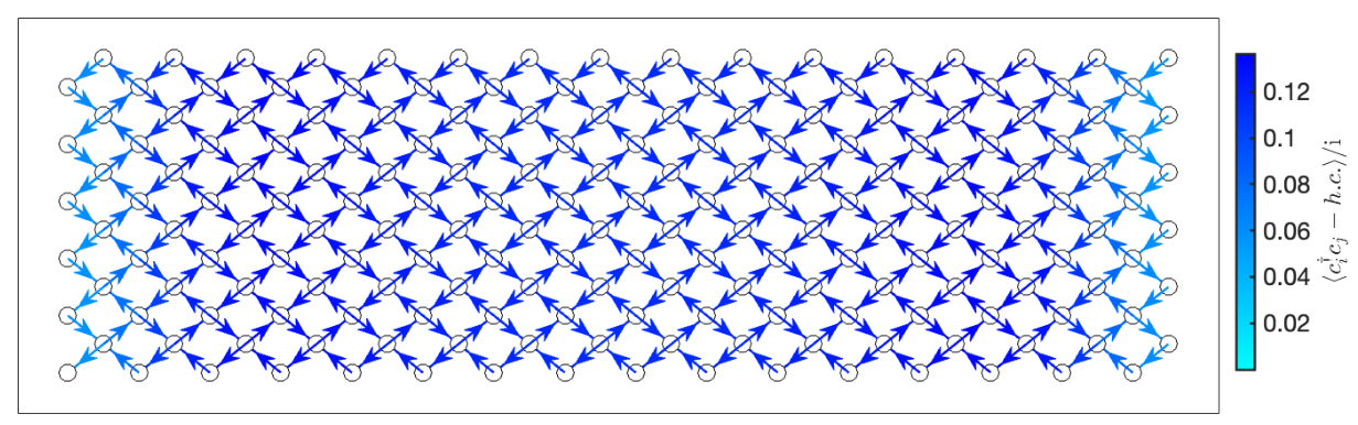
The exact loop current is plotted in Fig.S7, which further clearly supports the evidence of time-reversal symmetry breaking.
I.6 Section VI: Purified entanglement entropy
The entanglement entropy is measured from the partial trace of the “superdensity” matrix of the “superstate” , which vectorizes the MPO for .


As shown in Fig.S8, at low , the entanglement entropy is the highest for QAH (which might be due to the edge states), while much lower for the site-nematic insulator and stripe insulator. The bond-nematic dirac semimetal phase shows higher entanglement entropy than the site nematic insulator, and show clear phase boundaries at low temperature. Such entanglement data indicate a possible gapless state, which are in agreement with previous conclusions.
I.7 Section VII: DMRG results in BNDS
As the BNDS between stripe insulator and SNI has not been investigated before, we implement DMRG simulations to varify the dirac semimetal phase. Since the dirac points are not on the high-symmetry points in momentum space, we take the cylinder width to decrease the finite-size effect. We simulate the entanglment entropy in the BNDS region and fit it to the universal scaling function . We show the results in Fig.S9. With up to , the entanglement entropy is still not converged, with the fitted central charge as large as , which is shown in the main text and this is enough to support the gapless BNDS phase.
As shown in the main text, we have measured the single-particle gap with twisted-boundary conditions in BNDS phase with and . We define the gap , where is the ground state energy and is the lowest energy in the single-particle-excited sector of our DMRG simulations. We do extrapolations with different bond dimensions to obtain the energies as shown in Fig.S10;


I.8 Section VIII: Energy spectrum of mean field hamiltonian
For the mean field analysis, we write the hamiltonian as:
| (S6) |
From the tight-binding part of Eq. (1), we change NN hopping with the sign structure following the direction shown in Fig. 1(c) to mimic the QAH phase; For the bond order state, we change NNN hopping with positive , i.e. stronger hopping integral along vertical direction; For the site-nematic state, we add sublattice chemical potential term to the hamiltonian Eq. 1. we plot the energy spectrum as shown in Fig.S11. For the original tight-binding model, there is a QBT at (). In the QAH with finite NN loop current, the gap will open immediately. Besides, we estimate the mean-field gap in QAH through this effective hamiltonian. For example, when and , we have measured in our DMRG simulations that the ratio of NN bond current and NN hopping amplitude (measured to be around 0.18) is approximately 0.35, so we tune here and the gap is around 0.22, as shown in Fig.S11(b). When adding site nematic order or NNN bond nematic order into the hamiltonian, the QBT will split into two dirac touching points, and the larger the order, the farther are the two points [1,6]. If the two dirac points getting far enough (qualitatively in this model, ), the system will be gapped, while the bond nematic order itself cannot open the gap for this system and even when the bond-nematic order is almost the same as the NNN hopping amplitude in the hamiltonian, the moving distance of Dirac cones is less than .


As we have discussed in the main text, the NNN bond nematic order and site nematic order break the same symmetry, we show how they can induce each other in the mean-field level as shown in Fig.S12. Besides, when is large enough and the the system is gapped out, the bond nematic order will drop. When in the mean-field hamiltonian, the two Dirac points merge into each other and are about to gap out. At this point, the bond order drop most significantly.

I.9 Section IX: First-order transition between QAH and Stripe
To show more details of the transition between QAH and Stripe, we show the structure factors of the two phases at different temperature near their transition point in Fig.S13. It is clear that near the first-order transition point , suddenly drops while jumps to a high value from 0.
