Higher Order Gauge Equivariant CNNs on Riemannian Manifolds and Applications

Many applications in computer vision call for the analysis of signals sampled on an underlying manifold that is non-Euclidean. A ubiquitous example of such a non-Euclidean space is the 2-sphere $S^{2}$. Atmospheric signals such as temperature and wind fields, measurements of the cosmic microwave background, and omnidirectional images captured by fish-eye lenses are all examples of signals whose domain ought to be modeled by $S^{2}$. It is desirable for CNNs that process spherical signals to be equivariant to rotations, i.e. equivariant to the action of the Lie group $\mathsf{SO}(3)$. This is analogous to the translation equivariance satisfied by planar CNNs.

The need to generalize CNNs to homogeneous spaces such as $S^{2}$ and even arbitrary Riemannian manifolds has since been answered by a flurry of techniques arising from an emerging subfield known as geometric deep learning (GDL) [11]. Here we review but a fraction of the relevant GDL literature.

Previously published CNNs that are equivariant to 2D and 3D rotations were reported in [37, 35, 7] and [14, 15, 20, 25], respectively. More recently, work aimed at generalizing beyond the plane and sphere was reported in [26, 3, 16, 6], in which their networks can in theory cope with arbitrary homogeneous spaces. From here, group convolutions on homogeneous spaces were pushed further along two diverging research directions of relevance, which this paper sets out to merge together. In one direction, the higher order analogue (Volterra expansion) of convolution on homogeneous spaces was introduced in [2], in which the parameter efficiency of higher order convolutions was demonstrated. In the other direction, the condition of having a homogeneous base space was relaxed, giving rise to the gauge equivariant convolutions presented in [17, 18, 36] which are valid on arbitrary Riemannian manifolds. It is still valuable to consider gauge equivariant convolutions on homogeneous spaces, as they afford high spatial resolutions while maintaining feature maps of low bandwidth (yielding better computational/memory efficiency). This is in stark contrast to group convolutional techniques (à la Fourier), where the spatial resolution and feature map bandwidth are invariably coupled together.

Let $M$ be a connected, geodesically complete Riemannian manifold of dimension $2$. Recall that to each $p\in M$, we can associate the tangent space $T_{p}M$ and its dual $T_{p}^{*}M$ [27]. A feature map $f$ on $M$ is modeled as a smooth tensor field on $M$, i.e. $f(p)$ is a tensor for each $p\in M$. We denote this as $f(p)\in T_{p}M^{\otimes r}\otimes T_{p}^{*}M^{\otimes s}=:\mathfrak{T}M|_{p}$, where $\otimes$ denotes a tensor product and the superscript, ^⊗r, denotes an $r$-fold tensor product. A convolution will then map a tensor field $f_{\mathrm{in}}$ on $M$ to a tensor field $f_{\mathrm{out}}$ on $M$. The reason for working with tensor-valued features will be made explicit below.

A tensor field $f$ on $M$ is a geometrically intrinsic construction that in general will lack a canonical global coordinatization. Therefore, to perform computations, we must locally assign a frame to each tangent space $T_{p}M$, which then induces a frame on the corresponding tensor space $\mathfrak{T}M|_{p}$. Such an assignment is called a gauge, which is to be thought of as a (local) smoothly parameterized collection of linear isomorphisms $w_{p}:\mathbb{R}^{2}\longrightarrow T_{p}M$. Given a frame $\{b_{1},b_{2}\}$ on $\mathbb{R}^{2}$, $w_{p}$ induces a frame on $T_{p}M$ given by $\mathbf{e}_{1}=w_{p}(b_{1})$ and $\mathbf{e}_{2}=w_{p}(b_{2})$. Figure 1 illustrates this concept.

Since the choice of gauge is arbitrary, we are forced to consider the transition between gauges via a gauge transformation. At a point $p\in M$ with pointwise gauges $w_{p}:\mathbb{R}^{2}\longrightarrow T_{p}M$ and $\widetilde{w}_{p}:\mathbb{R}^{2}\longrightarrow T_{p}M$, this amounts to considering the map $t:=w_{p}^{-1}\circ\widetilde{w}_{p}$. The map $t$ acts naturally on frames and tangent vector coefficients, where in computations we use a corresponding change-of-basis matrix.

For example, if our feature map $f$ is a vector field, then $f(p)\in T_{p}M$. A tangent vector $f(p)=\mathbf{v}$ is an intrinsic geometric object, but we can coordinatize $\mathbf{v}$ with respect to the pointwise gauges $w_{p}$ and $\widetilde{w}_{p}$ above, yielding coordinates $w_{p}^{-1}(\mathbf{v})=a=(a_{1},a_{2})$ w.r.t. $\{\mathbf{e}_{1},\mathbf{e}_{2}\}$ and $\widetilde{w}_{p}^{-1}(\mathbf{v})=\widetilde{a}=(\widetilde{a}_{1},\widetilde{a}_{2})$ w.r.t. $\{\widetilde{\mathbf{e}}_{1},\widetilde{\mathbf{e}}_{2}\}$. Under the assumption that $\widetilde{w}_{p}=w_{p}\circ t$, it must be the case that $\widetilde{a}=t^{-1}(a)$, so that $\mathbf{v}=\widetilde{w}_{p}(\widetilde{a})=(w_{p}\circ t)(\widetilde{a})=(w_{p}\circ t\circ t^{-1})(a)=w_{p}(a)$ is coordinate independent. The relation $\widetilde{a}=t^{-1}(a)$ is referred to as a tensor transformation law, which describes how the coordinatization of a tensor changes w.r.t. a change of frame.

More generally, higher order tensors on a $2$-manifold have transformation laws of the form $\widetilde{a}=\rho(t^{-1})(a)$, where $\rho:G\longrightarrow\mathsf{GL}(2,\mathbb{R})$ is a group representation (i.e. $\rho(t_{1}t_{2})=\rho(t_{1})\rho(t_{2})$ for all $t_{1},t_{2}\in G$) and $G$ is a Lie subgroup of $\mathsf{GL}(2,\mathbb{R})$ called the structure group. As $\rho$ encodes the tensor transformation law, we also refer to $\rho$ as the tensor type. In this work, we are only interested in orthonormal frames with positive orientation, so we will only be concerned with $G=\mathsf{SO}(2)$ from here on out.

Since our feature maps are no longer scalar-valued and the base manifold is no longer Euclidean, there exist several differences between the classical convolution and the gauge equivariant convolution. Firstly, we must specify beforehand the tensor types $\rho_{\mathrm{in}}$ and $\rho_{\mathrm{out}}$ corresponding to the input and output of a convolution. Secondly, the kernel $K$ is upgraded to a smooth matrix-valued map $\mathbb{R}^{2}\longrightarrow\mathbb{R}^{d_{\mathrm{out}}\times d_{\mathrm{in}}}$ with compact support, where $d_{\mathrm{in}}$ and $d_{\mathrm{out}}$ are the dimensions of the tensor spaces $\mathfrak{T}_{\mathrm{in}}M|_{p}$ and $\mathfrak{T}_{\mathrm{out}}M|_{p}$ in which the input and output features lie, respectively. Thirdly, we must parallel transport the features in a given patch to a common tensor space so that operations such as feature addition become meaningful.

With these differences in mind, let $f_{\mathrm{in}}$ be a feature map of type $\rho_{\mathrm{in}}$ and $K:\mathbb{R}^{2}\longrightarrow\mathbb{R}^{d_{\mathrm{out}}\times d_{\mathrm{in}}}$ a kernel as above. We remind the reader that the Riemannian exponential map at a point $p\in M$ is a map $\operatorname{exp}_{p}:T_{p}M\longrightarrow M$ taking a tangent vector $\mathbf{v}\in T_{p}M$ to the point $\operatorname{exp}_{p}(\mathbf{v})\in M$ at which one arrives after following a geodesic with velocity $\mathbf{v}$ for one unit of time. Letting $q_{v}:=\mathrm{exp}_{p}(w_{p}v)$, the convolved feature map $f_{\mathrm{out}}=K\star f_{\mathrm{in}}$ is given pointwise by

where $t_{p\leftarrow q_{v}}$ denotes the $\mathsf{SO}(2)$-valued gauge transformation taking the frame on $q_{v}$ (after parallel transport to $p$) to the frame on $p$. Note that the action of $\rho_{\mathrm{in}}(t_{p\leftarrow q_{v}})$ on $f_{\mathrm{in}}(q_{v})$ subsumes the familiar translational shift $f(t-\tau)$ seen in the classical Euclidean convolution. In [17], it was shown that (1) is equivariant to a gauge transformation at $p$ if and only if $K$ is $\mathsf{SO}(2)$-steerable, i.e. $K$ satisfies

for all $t\in\mathsf{SO}(2)$ and $v\in\mathbb{R}^{2}$. It is crucial to note that in the case where $f_{\mathrm{in}}$ and $f_{\mathrm{out}}$ are scalar-valued feature maps, both $\rho_{\mathrm{in}}$ and $\rho_{\mathrm{out}}$ are trivial, meaning equation (2) reduces to $K(t^{-1}v)=K(v)$, i.e. we are constrained to isotropic kernels. This motivates the need to generalize to tensor-valued features so that we can detect anisotropy. We conclude with a critical result describing the relation between local equivariance w.r.t. gauge transformations and global equivariance w.r.t. isometries.

Hence, in particular, we have that gauge equivariant convolutions where $G=\mathsf{SO}(2)$ and $M=S^{2}$ are equivariant to global rotations $\phi\in\mathsf{SO}(3)$.

Convolutional kernel networks (CKNs) [28] are the culmination of merging traditional CNNs with kernel methods. In the CKN setting, a feature map at the $\ell^{\mathrm{th}}$ layer is modeled as a function $I_{\ell}:\Omega_{\ell}\longrightarrow\mathcal{H}_{\ell}$, where $\Omega_{\ell}$ is some Euclidean domain and $\mathcal{H}_{\ell}$ is a reproducing kernel Hilbert space (RKHS). As in any learning scheme that wishes to exploit the kernel trick, an appropriate positive definite kernel $K_{\ell}:\mathcal{X}_{\ell-1}\times\mathcal{X}_{\ell-1}\longrightarrow\mathbb{R}$ must be defined. We take $\mathcal{X}_{\ell}$ to be the space of image patches (of a fixed size) with support in $\Omega_{\ell}$ and $K_{\ell}(\mathbf{x},\mathbf{x}^{\prime}):=||\mathbf{x}||\,||\mathbf{x}^{\prime}||\,\kappa_{\ell}(\langle\frac{\mathbf{x}}{||\mathbf{x}||},\frac{\mathbf{x}^{\prime}}{||\mathbf{x}^{\prime}||}\rangle)$, where $\kappa_{\ell}$ is a nice $\mathbb{R}$-valued function. For instance, if we are dealing with $3\times 3$ patches of a 2D greyscale image, then $\mathcal{X}=\mathbb{R}^{3\cdot 3\cdot 1}=\mathbb{R}^{9}$. Recall that a positive definite kernel $K_{\ell}$ induces an embedding $\varphi_{\ell}(\mathbf{x})=K_{\ell}(\mathbf{x},-)$ taking image patches $\mathbf{x}\in\mathcal{X}_{\ell-1}$ into the RKHS $\mathcal{H}_{\ell}$. Instead of learning a set of weights, a CKN learns a finite-dimensional subspace $\mathcal{F}_{\ell}\subset\mathcal{H}_{\ell}$ for each $\ell$ such that the projection residuals (projection onto $\mathcal{F}_{\ell}$) of the embedded $\varphi_{\ell}(\mathbf{x})$ are minimized. The ability to choose $\kappa_{\ell}$ to our liking is the main property of CKNs that we will leverage in 3.2.

Let $M$ be a connected, geodesically complete Riemannian 2-manifold as before. We avoid unnecessary generalization by maintaining that $G=\mathsf{SO}(2)$. However, the following definitions and results can be modified for arbitrary structure groups $G\subseteq\mathsf{GL}(2,\mathbb{R})$.

We are now ready to present a theorem on the gauge equivariance of the higher order operator $V_{\mathcal{K}}^{m}$. Such a result is necessary for two reasons: (a) we would like for the output of $V_{\mathcal{K}}^{m}$ to be independent of the coordinatization of its input and (b) we want $V_{\mathcal{K}}^{m}$ to further enjoy $\mathsf{SO}(3)$-equivariance in the case where $M=S^{2}$ (cf. Theorem 2.1).

In any application of steerable kernels, the main difficulty arises from generating solutions to the steerability constraint [35], which is usually done via some combination of analytic and representation-theoretic methods. The most desirable outcome is to obtain a complete basis for the subspace of kernels that are steerable. Our use case will only involve second order expansions of vector-valued feature maps, and thus we make do with the following sufficient condition on second order $\mathsf{SO}(2)$-steerable kernels.

Using Proposition 3.5, we can generate a set $\mathcal{B}$ of second order $\mathsf{SO}(2)$-steerable kernels from the first order solutions obtained in [35] to map $\rho_{1}$ features to $\rho_{1}$ features. Note that 3.5 can be modified to account for the other relevant cases (e.g. $\rho_{1}\to\rho_{0}$, etc.). We then parameterize the space of second order $\mathsf{SO}(2)$-steerable kernels w.r.t $\mathcal{B}$, learning only the scalar coefficients.

The traditional convolution operator $H_{1}$ admits a natural generalization called the Volterra series operator [34], which for $1$-dimensional signals $f(x)$ is given by $Vf(x)=\sum_{k=0}^{\infty}H_{k}f(x)$, where

and $H_{0}$ is some constant. Note how Definition 5 reduces to (6) in the case of scalar-valued feature maps on Euclidean space. The higher order terms ($k>1$) can model nonlinear interactions within a given receptive field [2, 40]. The problem with directly applying equation (6) is that higher order cross-correlations quickly become computationally intractable as we increase the dimension of the input signals and the degree of the expansion. Moreover, the Volterra kernels $h^{(k)}$ contain many redundancies in the typical case where we assume $h^{(k)}$ to be symmetric, i.e. $h^{(k)}(\tau_{1},\ldots,\tau_{k})=h^{(k)}(\tau_{\sigma(1)},\ldots,\tau_{\sigma(k)})$ for any permutation $\sigma$.

Kernel methods offer a solution to these issues. In [22], it was shown that the estimation of $V^{(m)}f(x)=\sum_{k=0}^{m}H_{k}f(x)$ is equivalent to optimizing against the hypothesis $\widehat{V}^{(m)}f(x)=\sum_{j=1}^{N}\gamma_{j}k^{(m)}(f(x),f(x_{j}))$, where $N$ is the number of training samples, $\gamma_{j}$ are learnable coefficients, $x_{j}$ is the $j^{\mathrm{th}}$ training sample, and $k^{(m)}$ is a reproducing kernel of the form $k^{(m)}(f(x_{1}),f(x_{2}))=(c+f(x_{1})^{\top}f(x_{2}))^{m}$, for some constant $c$. Since we would like $f(x)$ to be representative of an entire dMRI volume, we hierarchically construct the features $f(x_{j})$ using the CKN formulation given in 2.2 with polynomial kernels $\kappa_{\ell}$. This yields an end-to-end implementation of an (approximate) $m^{\mathrm{th}}$ order Volterra expansion for arbitrary $m$ that relies on the same number of learnable parameters as would a first order CNN, since the only modification we make is to the degree of $\kappa_{\ell}$.

The spherical MNIST data were generated using the code released in [15], except we project onto an icospherical grid instead of a Driscoll-Healy grid. Nevertheless, the original input resolutions are comparable. There are three variations of the dataset, namely NR/NR, NR/R, and R/R, where for example NR/R means that the training data has not been rotated post-projection while the test data has been randomly rotated.

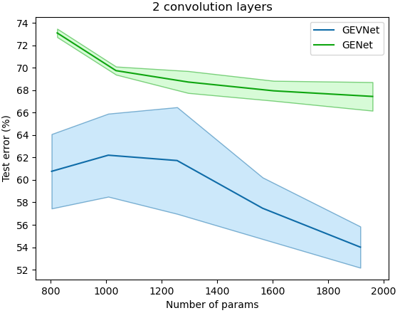
To begin, we compare the test performance of a second order GEVNet versus that of a first order GENet on NR/NR while varying the number of learnable parameters in each model. We consider three cases: 2-, 3- and 4-layer networks (see appendix for 3 and 4 layers), where for each case we initialize five GEVNet models and five GENet models with progressively increasing parameter counts to compare the trends in classification error. For each choice of GEVNet architecture, we ensure that there is a corresponding GENet with at least as many learnable parameters. For instance, to a 2-layer GEVNet (804 params) with architecture $\operatorname{\mathbf{GEVConv}}(1^{\rho_{0}},2^{\rho_{0}\oplus\rho_{1}})^{\downarrow}\rightarrow\operatorname{\mathbf{GEVConv}}(2^{\rho_{0}\oplus\rho_{1}},2^{\rho_{0}})$ we associate a 2-layer GENet (824 params) with architecture $\operatorname{\mathbf{GEConv}}(1^{\rho_{0}},2^{\rho_{0}\oplus\rho_{1}})^{\downarrow}\rightarrow\operatorname{\mathbf{GEConv}}(2^{\rho_{0}\oplus\rho_{1}},4^{\rho_{0}})$. Such a constraint can be seen as adversarial against GEVNets. For a given number of layers, all models are trained using the same optimization hyperparameters and for the same duration (20 epochs). The plot in Figure 3 reports mean test errors across five runs per model and shaded regions convey the standard error of the mean (95% confidence). Note how in all cases the GEVNet’s test error is consistently lower than the GENet’s as we vary parameter counts. This suggests that the GEVNet produces a richer class of features in comparision to a GENet for the same number of learnable parameters.

Finally, in Table 2 we report our best GEVNet model on the standard spherical MNIST benchmarks in comparison to previous works. Our model achieves comparable performances for a far fewer number of parameters than other spherical CNNs.

Here we consider the application of a GEVNet to the benchmark QM7 dataset [10, 32], with the goal of regressing atomization energies of molecules given their consituent atoms’ positions and charges. Our setup is identical to that of [15], using a rotation and translation invariant Coulomb matrix representation. We present our result in Table 2. We come in second in RMSE but at a significant reduction of parameters in comparison to all other models.

Data Description: The dMRI data pool we used consisted of brain scans from 85 patients with Lewy Body Disease (DLB), 112 patients with Alzheimer’s Disease (AD) and 436 patients with Parkinson’s Disease (PD). All the scans were first axis aligned, centered, eddy current corrected, and brain extracted using FSL and pnlNipype [1, 8]. Since the data were pooled from different magnetic resonance (MR) scanners (Siemens 3T, GE 3T, and Philips 3T) possessing distinct acquisition parameters, the scans underwent a retrospective harmonization step to increase inter-scanner compatability. This was done using the publicly available dMRI harmonization software in [9, 23]. After harmonization, the scans were affinely registered to a common MNI (Montreal Neurological Institute) space and downsampled to a voxel size of 2 mm³. Finally, the image intensities at a given voxel (to be thought of as a scalar field on $S^{2}$) were passed through a spherical (radial basis function) interpolation and re-sampled onto a Healpix grid [19] with 192 grid points. This corresponds to 96 distinct magnetic field gradient directions due to antipodal symmetry.

Since the amount of raw data is relatively small (especially for AD and DLB), we set up five (80/20 split) train/test folds for each of the three possible classification problems (AD v. DLB, AD v. PD, and DLB v. PD) to obtain averaged performance estimates. To mitigate class imbalance, we then augment each training set using a data synthesis technique called mixup [38] such that there are 400 training samples per class.

Network Architecture: An input dMRI volume can be seen as 4-dimensional, consisting of a 3D MRI for each diffusion-sensitized gradient direction (i.e. for each $b$-vector). A $b$-vector is the vector pointing in the direction of the applied diffusion-sensitized magnetic field gradient. Alternatively, one can think of a dMRI volume as a 3D lattice, where at each lattice point (voxel) we have a scalar field on $S^{2}$.

With this in mind, the data flow for a single dMRI volume is as follows: (1) each 3D volume (corresponding to a given $b$-vector) is passed as input to a CKN whose domain is $\mathbb{R}^{3}$, which summarizes diffusion phenomena occurring across voxels, (2) the resulting feature maps are concatenated along a fourth dimension, (3) each scalar field (on $S^{2}$) is passed to a spherical CNN, thus extracting a feature vector that is representative of the intra-voxel diffusion, (4) obtain a single feature vector by global average pooling, and (5) the final feature vector is classified by a fully connected block. Steps 1 and 2 are easily implemented in PyTorch by letting the $b$-vector dimension be the batch dimension. Then, we swap the batch and spatial dimensions before step 3 since the $b$-vector directions become the grid positions on $S^{2}$. Figure 4 depicts a schematic of this network. Our CKN implementation is an adaptation of [12].

Ablation Study: We test the effect of higher order convolutions on three neurodegenerative disorder classification problems: AD v. DLB, AD v. PD, and DLB v. PD. Ablation is performed on the order of the inter-voxel convolution (CKN) by varying the degree of a polynomial kernel, and on the order of the intra-voxel convolution (spherical CNN) by exchanging a second order GEVNet with a first order DeepSphere (DS) [19]. The abbreviations CKN1 and CKN2 refer to a CKN with linear and quadratic kernels, respectively. Although not identical, a CKN1 can be viewed as a close approximation to a standard CNN. We also include two additional ablated models: a lone CKN2 that ignores diffusion-sensitized gradient directions by flattening the feature map after the last layer, and a lone GEVNet that ignores diffusion phenomena across voxels.

Each CKN has a fixed architecture consisting of a mere 3164 learnable parameters. Both the GEVNet and the DeepSphere consist of three convolution layers, with the GEVNet having 12424 parameters and the DeepSphere having 13696 parameters. All other optimization-related hyperparameters (e.g. learning rate, weight decay, number of epochs) are kept the same across classification tasks, and are provided in detail in the appendix. The test accuracies (averaged over five train/test folds) are presented in Table 3.

For a fixed choice of CKN, we find that an accompanying GEVNet outperforms its DS counterpart by a significant margin, except in the case of CKN2 + GEVNet versus CKN2 + DS on DLB v. PD, where the accuracies are highly comparable. This is significant, given that the GEVNet is at an over 1k parameter disadvantage against the DeepSphere. We attribute the exceptional case to the observation that a lone CKN2 is already enough to discriminate DLB v. PD with above 98% accuracy, leaving little to be gained by a spherical component. Said differently, this suggests that DLB and PD are distinct enough to be separated by macroscale volumetric features, as opposed to microscale diffusion features. Conversely, for a fixed choice of spherical CNN, we find that replacing the accompanying CKN’s linear kernel with a quadratic kernel yields a boost in performance. Thus, we see that CKN2 + GEVNet is the overall best classifier, as it performs second order convolutions both across and within voxels.

Proposition 3.5 allows us to generate second order $\mathsf{SO}(2)$-steerable basis kernels from the first order solutions obtained in [35]. For example, we can construct the (angular) second order basis kernel of type $(\rho_{1},\rho_{1})$ given by

We begin by presenting additional plots depicting our ablation study on parameter counts (Figure 5). Note that the plots presented here depict the statistics (mean error and standard error of the mean) obtained over 10 runs per model. Again, we find that the GEVNet exhibits greater representational capacity than its first order analogue in all cases. All models for the ablation study were trained for 20 epochs, with an exponentially decaying initial learning rate of $3\mathrm{e}{-}4$. All regular nonlinearities mapped the hidden feature vectors to $N=101$ spatial samples, and the precomputed basis kernels were homogenized using a single ring consisting of 1000 quadrature points. We used a batch size of 512, cross entropy loss, and an ADAM optimizer.

Next, we present the details of the reported GEVNet and GENet architectures on the MNIST benchmark tasks. The GEVNet’s architecture (31k params) is given by

while the GENet’s architecture (45k params) is given by

Both models were trained for 30 epochs, with an exponentially decaying initial learning rate of $1\mathrm{e}{-}4$. Regular nonlinearities mapped the hidden feature vectors to $N=51$ spatial samples, and the precomputed basis kernels were homogenized using a single ring consisting of 1000 quadrature points. We used a batch size of 256, cross entropy loss, and an ADAM optimizer.

All MNIST experiments were performed on a single NVIDIA A100 GPU.

As described in [15], this task is handled by an architecture consisting of a spherical component followed by an MLP. We do not modify the original MLP in any way, only substituting Cohen’s $S^{2}$CNN with our GEVNet. The GEVNet’s architecture is given by

The model was trained for 30 epochs with a learning rate of $1\mathrm{e}{-}3$ and a weight decay of $1\mathrm{e}{-}2$ using a batch size of 16, MSE loss, and an ADAM optimizer. All regular non-linearities mapped the hidden feature vectors to $N=101$ spatial samples, and the precomputed basis kernels were homogenized using a single ring consisting of 1000 quadrature points. This experiment was performed on a single NVIDIA A100 GPU.

All compound models depicted in Table 3 of the main paper were trained for 15 epochs, with an exponentially decaying initial learning rate of $1\mathrm{e}{-}5$ and a weight decay of $1\mathrm{e}{-}5$ using cross entropy loss and an ADAM optimizer. All regular non-linearities mapped the hidden feature vectors to $N=7$ spatial samples, and the precomputed basis kernels were homogenized using a single ring consisting of 5000 quadrature points. Given the large input image size (approx. 563k voxels), we parallelize the training across 6 NVIDIA A100 GPUs while taking care to use a synchronized batch normalization. The reported DeepSphere’s architecture was given by

References

- [1] J.L.R. Andersson and S.N. Sotiropoulos. An integrated approach to correction for off-resonance effects and subject movement in diffusion MR imaging. Neuroimage, 125:1063–1078, 2016.
- [2] M. Banerjee, R. Chakraborty, J. Bouza, and B.C. Vemuri. VolterraNet: A higher order convolutional network with group equivariance for homogeneous manifolds. IEEE TPAMI, 44(2):823–33, 2022.
- [3] M. Banerjee, R. Chakraborty, et al. DMR-CNN: A CNN tailored for DMR scans with applications to PD classification. In 16th IEEE ISBI, pages 388–391. IEEE, 2019.
- [4] M. Banerjee, R. Chakraborty, E. Ofori, et al. A nonlinear regression technique for manifold valued data with applications to Medical Image Analysis. In The IEEE Conf. on CVPR, 2016.
- [5] P.J. Basser, J. Mattiello, and D. LeBihan. MR diffusion tensor spectroscopy and imaging. Biophysical Journal, 66(1):259—267, January 1994.
- [6] E.J. Bekkers. B-Spline CNNs on Lie Groups. In International Conference on Learning Representations, 2020.
- [7] E.J. Bekkers, M.W. Lafarge, M. Veta, et al. Roto-Translation Covariant Convolutional Networks for Medical Image Analysis. In Medical Image Computing and Computer Assisted Intervention – MICCAI 2018, pages 440–448. Springer International Publishing, 2018.
- [8] T.C. Billah, S. Bouix, and Y. Rathi. NIFTI MRI preprocessing pipeline, 2019. URL: https://github.com/pnlbwh/pnlNipype.
- [9] T.C. Billah, S.C. Karayumak, S Bouix, and Y. Rathi. Multi-site dMRI harmonization, 2019. URL: https://github.com/pnlbwh/dMRIharmoniziation.
- [10] L.C. Blum and J. Reymond. 970 Million Druglike Small Molecules for Virtual Screening in the Chemical Universe Database GDB-13. Journal of the American Chemical Society, 131(25):8732–8733, 2009.
- [11] M.M. Bronstein, J. Bruna, T. Cohen, and P. Velickovic. Geometric Deep Learning: Grids, Groups, Graphs, Geodesics, and Gauges. CoRR, 2021. arXiv:2104.13478.
- [12] Dexiong Chen. Convolutional kernel network with pytorch. https://github.com/claying/CKN-Pytorch-image, 2019.
- [13] O. Cobb, C.G.R. Wallis, A.N. Mavor-Parker, et al. Efficient Generalized Spherical CNNs. In International Conference on Learning Representations, 2021.
- [14] T.S. Cohen, M. Geiger, J. Koehler, and M. Welling. Convolutional Networks for Spherical Signals. In Proceedings of ICML. JMLR, 2017.
- [15] T.S. Cohen, M. Geiger, J. Koehler, and M. Welling. Spherical CNNs. In Proceedings of ICLR. JMLR, 2018.
- [16] T.S. Cohen, Mario Geiger, and Maurice Weiler. A General Theory of Equivariant CNNs on Homogeneous Spaces. In Advances in Neural Information Processing Systems 32: Annual Conference on Neural Information Processing Systems, pages 9142–9153, 2019.
- [17] T.S. Cohen, M. Weiler, B. Kicanaoglu, and M. Welling. Gauge Equivariant Convolutional Networks and the Icosahedral CNN. In Proc. of the 36th ICML, volume 97 of Proc. of ML Research, pages 1321–1330. PMLR, 2019.
- [18] P. de Haan, M. Weiler, T.S. Cohen, and M. Welling. Gauge Equivariant Mesh CNNs: Anisotropic convolutions on geometric graphs. In International Conference on Learning Representations, 2021.
- [19] M. Defferrard, M. Milani, F. Gusset, and N. Perraudin. DeepSphere: a graph-based spherical CNN. In International Conference on Learning Representations (ICLR), 2020.
- [20] C. Esteves, C. Allen-Blanchette, X. Zhou, and K. Daniilidis. Polar Transformer Networks. In International Conference on Learning Representations, 2018.
- [21] C. Esteves, A. Makadia, and K. Daniilidis. Spin-Weighted Spherical CNNs. In Advances in Neural Information Processing Systems, volume 33, pages 8614–8625, 2020.
- [22] M.O. Franz and B. Schölkopf. A Unifying View of Wiener and Volterra Theory and Polynomial Kernel Regression. Neural Computation, 18(12):3097–3118, 2006.
- [23] S.C. Karayumak, S. Bouix, L. Ning, et al. Retrospective harmonization of multi-site diffusion MRI data acquired with different acquisition parameters. Neuroimage, 184:180–200, 2019.
- [24] B. Kicanaoglu, P. de Haan, and T.S. Cohen. Gauge Equivariant Spherical CNNs. 2020. URL: https://openreview.net/forum?id=HJeYSxHFDS.
- [25] R. Kondor, Z. Lin, and S. Trivedi. Clebsch–Gordan Nets: a Fully Fourier Space Spherical Convolutional Neural Network. In Advances in Neural Information Processing Systems, volume 31, 2018.
- [26] R. Kondor and S. Trivedi. On the Generalization of Equivariance and Convolution in Neural Networks to the Action of Compact Groups. In Proceedings of ICML, 2018.
- [27] J.M. Lee. Riemannian Manifolds: An Introduction to Curvature. Springer-Verlag New York, Inc., New York, NY, 1997.
- [28] J. Mairal. End-to-End Kernel Learning with Supervised Convolutional Kernel Networks. In Proc. of the Intl. Conf. on NIPS, 2016.
- [29] E. Özarslan, B.C. Vemuri, and T.H. Mareci. Generalized scalar measures for diffusion MRI using trace, variance, and entropy. Magnetic Resonance in Medicine, 53(4):866–876, 2006.
- [30] O. Pasternak, N. Sochen, Y. Gur, et al. Free water elimination and mapping from diffusion MRI. Magnetic Resonance in Medicine (MRM), 62(3):717–730, 2009.
- [31] J. Prodoehl, H. Li, P.J. Planetta, et al. Diffusion tensor imaging of Parkinson’s disease, atypical parkinsonism, and essential tremor. Movement Disorders, 2013.
- [32] M. Rupp, A. Tkatchenko, K. Müller, and A. Von Lilienfeld. Fast and Accurate Modeling of Molecular Atomization energies with Machine Learning. Physical Review Letters, 108(5):058301, 2012.
- [33] A.J. Thomas, J.P. Taylor, I. McKeith, et al. Development of assessment toolkits for improving the diagnosis of the Lewy body dementias: feasibility study within the DIAMOND Lewy study. International Journal of Geriatric Psychiatry, 32:1280–1304, 2017.
- [34] V. Volterra. Theory of Functionals and of Integral and Integro-Differential Equations. 1930.
- [35] M. Weiler and G. Cesa. General E(2)-Equivariant Steerable CNNs. In Proc. of the Intl. Conf. on NIPS, 2019.
- [36] M. Weiler, P. Forré, E. Verlinde, and M. Welling. Coordinate Independent Convolutional Networks – Isometry and Gauge Equivariant Convolutions on Riemannian Manifolds, 2021. URL: https://arxiv.org/pdf/2106.06020.pdf.
- [37] D.E. Worrall, S.J. Garbin, D. Turmukhambetov, and G.J. Brostow. Harmonic Networks: Deep Translation and Rotation Equivariance. In Proc. of the IEEE CVPR, pages 5026–5037. IEEE, 2017.
- [38] H. Zhang, M. Cisse, Y.N. Dauphin, and D. Lopez-Paz. mixup: Beyond Empirical Risk Minimization. In Intl. Conf. on ICLR, 2018.
- [39] H. Zhang, T. Schneider, C.A. Wheeler-Kingshott, and D.C. Alexander. NODDI: practical in vivo neurite orientation dispersion and density imaging of the human brain. Neuroimage, 61(4):1000–1016, 2012.
- [40] G. Zoumpourlis, A. Doumanoglou, N. Vretos, and P. Daras. Non-linear Convolution Filters for CNN-based Learning. In Proc. of ICCV, pages 4771–4779. IEEE, 2017.
A Theory
We use the same notation as described in the body of the paper, but we reiterate it here for convenience. denotes the order expansion of a feature map , whose definition entails convolutions of with a collection of -steerable kernels , where indicates the order of the kernel. is a group homomorphism that encodes the transformation law of the feature map ’s coordinatization under -valued gauge transformations, where is the dimension of the tensor spaces in which individual features lie. Finally, we let for a gauge , and denotes the -valued gauge transformation taking the parallel transported frame at to the frame at .
A.1 Proof of Theorem 3.4
Theorem 3.4.
is gauge equivariant. That is, if and are two pointwise gauges at related by an -valued gauge transformation , then transforms as .
Proof.
By linearity, it suffices to show that is gauge equivariant for each . Let us embellish any coordinate dependent object with a when written w.r.t. . Assuming an initial coordinatization w.r.t. , we have that
Note that no modification needs to be made to the integration measure under a gauge transformation since for all . ∎
A.2 Proof of Proposition 3.5
Proposition 3.5.
Let be a first order -steerable kernel of type and a first order -steerable kernel of type , where is the trivial representation (i.e. ) and is the standard representation mapping to the usual rotation matrix. Then, a second order kernel of the form is -steerable of type .
Recall the mixed-product property: given matrices , , , and (of compatible sizes), we have that . Letting and letting MP denote the mixed-product property, we have that