Optimal separator for an hyperbola
Application to localization

Consider an equation of the form

The pair of transformations $(\sigma,\gamma)$ is conjugate with respect to $f$ if

Transformations that will be consider are limited to the hyperoctahedral group $B_{n}$ [3] which is the group of symmetries of the hypercube $[-1,1]^{n}$ of $\mathbb{R}^{n}$. The group $B_{n}$ corresponds to the group of $n\times n$ orthogonal matrices whose entries are integers. Each line and each column of a matrix should contain one and only one non zero entry which should be either $1$ or $-1$. Figure 1 shows different notations usually considered to represent a symmetry $\sigma$ of $B_{5}$. We will prefer the Cauchy one line notation [20] which is shorter. We should understand the symmetry $\sigma$ of the figure as the function:

In the plane, the group $B_{2}$ has eight elements. If we use the matrix form, the elements of $B_{2}$ are

Equivalently with the Cauchy notation, these 8 elements of $B_{2}$ are respectively

A symmetry of $B_{2}$ in a matrix form, satisfies

with $\sigma_{ij}^{2}\in\{0,1\},\sigma_{i1}^{2}+\sigma_{i2}^{2}=1,\sigma_{1j}^{2}+\sigma_{1j}^{2}=1.$ The Cauchy form is obtained from the matrix form by left multiplying by the line vector $(1,2):$

The following theorem gives the symmetries of the hyperbola.

Considering Proposition 0.1, we get the choice function $\psi$ [9]:

where $\alpha=\sigma^{-1}$. Given a symmetry $\sigma$, this choice function allows us to get a symmetry $\gamma$ such that $(\sigma,\gamma)$ is a conjugate pair.

For instance $\mathbf{e}_{3}=(0,0,1,0)^{\text{T}}$ and $\mathbf{e}{}_{-2}=(0,-1,0,0)$ are two cardinal vectors of $\mathbb{R}^{4}$. We use the notation $\mathbf{e}_{i}$ where $i\in I=\{-n,\dots,-1,1,\dots,n\}$ to specify the cardinal vector. For instance $\mathbf{e}{}_{-2}$ is the vector parallel to the $2$ axis with a negative direction.

Figure 2 shows in case of $n=2$, a representation of the functions $\varphi_{1}(x_{2})$ (red) and $\varphi_{-1}(x_{2})$ (blue). The small squares correspond to cardinal points (East in red and West in blue). Here, we have two Easts and two Wests.

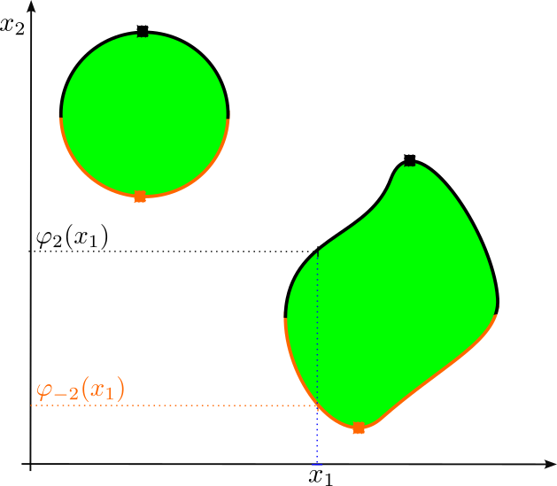
Figure 3 is a representation of the functions $\varphi_{2}(x_{1})$ (black) and $\varphi_{-2}(x_{1})$ (orange). The small squares correspond to cardinal points (North in black and South in orange).

In Figure 2, we observe that graphs of the function $\varphi_{1}$ and $\varphi_{-1}$ do not cover the boundary of $\mathbb{X}$. This is due to the fact that $\mathbb{X}$ is not row convex. We define the notion of row convexity (similar to the definition in [19])

For the hyperbola defined by

We have four cardinal functions $\varphi_{i},i\in\{-2,-1,1,2\}.$ As it will be shown, the hyperbola is row convex and its cardinal functions will be sufficient to completely represent the equation.

To find $\varphi_{1}$, we fix $x_{2}$ and we search for the maximal value for $x_{1}$. The procedure leads to the following proposition. Other cardinal functions will be obtained by symmetries.

For instance a North belongs to the graphs of $\varphi_{1},\varphi_{-1},\varphi_{2}$ and a East belongs to the graphs of $\varphi_{2},\varphi_{-2},\varphi_{1}$. For our hyperbola we easily find that there exist four cardinal points. Of course, the cardinal points depend on $\mathbf{q}$.

Note that if the square root is not defined, then there is no cardinal points.

Corollary. Consider the hyperbola $f(\mathbf{q},\mathbf{x})=0$. Take the symmetry $\sigma=(1,3,2,6,5,4)$ and set $[x_{1}]=\rho(\sigma(\mathbf{q})$), the East of the hyperbola is $(x_{1}^{-},\varphi_{2}(x_{1}^{-}))$ and the West is $(x_{1}^{+},\varphi_{2}(x_{1}^{+}))$.

Let us assume that $\mathbf{q}$ is fixed. The dependency with respect to the parameter vector $\mathbf{q}$ will omitted for simplicity. As defined in the book of Moore [14], the interval extension function of $\varphi_{1}(x_{2})$ is

which returns the smallest interval which contains the set $\varphi_{1}([x_{2}])$. The same definition applies for other cardinal directions to get $[\varphi_{-1}]([x_{2}]),[\varphi_{2}]([x_{1}])$ and $[\varphi_{-2}]([x_{1}])$.

Due to the monotonicity of $\varphi_{1}$ between the cardinal points, we have

where $\mathbf{c}(1),\mathbf{c}(2),\dots$ are the cardinal points inside the box $[-\infty,\infty]\times[x_{2}]$.

Take for instance $\mathbf{q}=(-1,5,2,-2,30,-2)$, i.e.,

For an interval sampling $[x_{2}]=\frac{1}{5}\cdot[k,k+1]$, $k\in\mathbb{N}$, the function $[\varphi_{1}]([x_{2}])$ generates the red boxes of Figure 4. If we do the same for $[\varphi_{-1}]([x_{2}])$, we get the blue boxes. The small black square corresponds to the North and the small orange square corresponds to the South.

For a similar sampling along $x_{1}$, Figure 5 represents $[\varphi_{2}]([x_{1}])$ (black) and $[\varphi_{-2}]([x_{1}])$ (orange). The small blue square corresponds to the East and the small red square corresponds to the West. Note that here, the West is on the left of the East. This is never the case for an ellipse.

From the interval evaluation, we can build a contractor for the set $x_{1}=\varphi_{1}(x_{2})$. It is is given by

This contractor will be called a seed contractor because it will be used to construct all other contractors using symmetries. The contractor (29) is not minimal. It is only minimal with respect to $x_{1}.$ Since this contractor depends on $\mathbf{q}$, we will write $C_{0}^{\mathbf{q}}.$

We understand that $C_{0}^{\mathbf{q}}$ corresponds to a small portion of the hyperbola. The main challenge is now to build the the separator for the whole hyperbola using the single parametric contractor $C_{0}^{\mathbf{q}}$ and symmetries. Of course, we could add some other seed contractors, but our idea is to factorize the implementation as much as possible to avoid bugs and make the code adaptable to other types of sets.

We have a contractor $C_{0}^{\mathbf{q}}$ which is minimal in the direction of $x_{2}$. Recall that $C_{0}^{\mathbf{q}}([\mathbf{x}])$ contracts the box $[\mathbf{x}]$ with respect to a small portion of the hyperbola. Using the notion of contractor action [7], we show how we can extend this contractor $C_{0}^{\mathbf{q}}$ to other portions. We recall that the action of a symmetry $\sigma$ to the contractor $C$ is defined by

This means that $\sigma\bullet C$ is a contractor that has been built from the contractor $C$ as follows:

• •

  Apply to the box $[\mathbf{x}]$ the symmetry $\sigma^{-1}$

• •

  Apply the contractor $C$

• •

  Apply to the resulting box $C\circ\sigma^{-1}([\mathbf{x}])$ the symmetry $\sigma$.

For the hyperbola, we can make a partition of the curve into four portions :

• •

  North-East : $\mathbb{X}^{(1,2)}=\{(x_{1},x_{2}|x_{1}=\varphi_{1}(x_{2})\text{ and $x_{2}=\varphi_{2}(x_{1})$}\}$

• •

  North-West : $\mathbb{X}^{(1,-2)}=\{(x_{1},x_{2}|x_{1}=\varphi_{1}(x_{2})\text{ and $x_{2}=\varphi_{-2}(x_{1})$}\}$

• •

  South-East : $\mathbb{X}^{(-1,2)}=\{(x_{1},x_{2}|x_{1}=\varphi_{-1}(x_{2})\text{ and $x_{2}=\varphi_{2}(x_{1})$}\}$

• •

  South-West : $\mathbb{X}^{(-1,2)}=\{(x_{1},x_{2}|x_{1}=\varphi_{-1}(x_{2})\text{ and $x_{2}=\varphi_{-2}(x_{1})$}\}$

If we consider the pair $(\sigma,\gamma)$ conjugate with respect to the hyperbola, the contractor $\sigma\bullet C_{0}^{\psi_{\sigma}(\mathbf{q})}$ is associated to another portion of the hyperbola. For a given $\sigma$, the selection of the symmetries $\gamma$ such that $(\sigma,\gamma)$ is conjugate is made using the choice function (16). These symmetries can be understood geometrically but can also be computed automatically as shown in [7].

To understand the construction, consider the symmetry $\sigma=(2,1)\in B_{2}$. The contractor associated to $\mathbb{X}^{(1,2)}$:

It is minimal with respect to both directions $x_{1}$ and $x_{2}$ as illustrated by Figure 6. Note that the North-East portion is delimited by the two cardinal points North (black square) and East (red square). This is consistent with the fact that $\mathbb{X}^{(1,2)}$ corresponds to the North-East portion.

The following proposition shows that the contractor for the hyperbola can be expressed by a simple formula involving symmetries and the unique seed contractor $C_{0}^{\mathbf{q}}$. Getting such a formula will ease the implementation of the contractor.

Figure 7 illustrates the minimality of the contractor for the hyperbola.

This section proposes an optimal separator for an hyperbola area defined by

This separator is then used by a paver to compute boxes that are inside or outside the solution set.

As shown in [10], from a contractor on the boundary of a set $\mathbb{X}$ and a test for $\mathbb{X}$, we can obtain a separator. As a consequence, we can get an inner and an outer approximations for $\mathbb{X}$ as illustrated by Figure 8 for $\mathbf{q}=(-1,5,2,-2,30,-2)^{\text{$T$}}.$ The magenta boxes are proved to be inside $\mathbb{X}$ and the blue boxes are outside $\mathbb{X}.$ The accuracy is taken as $\varepsilon=0.1$ and corresponds to the size of the small uncertain boxes (yellow). The cardinal points (North, South, West, East) are represented by the small squares (black, orange, blue, red).

Figure 9 corresponds to the approximation obtained with the same accuracy with a classical forward-backward contractor. The benefice of our method seems small, but we will see later, that the improvement can become significant when the components of $\mathbf{q}$ are larger.

For $\mathbf{q}=(-1,1,1,3,30,-2)$ we only have two cardinal points (West and East). The formula provided by Proposition 0.4 is still valid and we are able to generate Figure 10. This shows the ability of the symmetries to consider different situations easily, elegantly and safely.

In this subsection, we show that an equation involving pseudo-distances corresponds to an hyperbola.

We consider an example taken from [6] related to localization which can be seen as special case of interval data fitting problem [13]. Consider a robot which emits a sound at an unknown time $t_{0}$. This sound is received with a delay by three microphones located points $\mathbf{a}:(13,7),\mathbf{b}:(4,6),\mathbf{c}:(16,10)$ of the plane (see Figure 11). Taking into account the time of flight of the sound we want to estimate the position of the object.

We have

where $c$ is the sound speed and $t_{a},t_{b},t_{c}$ is the detection time for microphones $\mathbf{a},\mathbf{b},\mathbf{c}$. We eliminate $t_{0}$ which is unknown to get

The quantity $\ell_{ab},\ell_{bc}$ are called pseudo-distances. We assume that we were able to measure the two pseudo distances to get $\ell_{ab}\in[7.9,8.1]$ and $\ell_{ac}\in[3.9,4.1]$. The set $\mathbb{X}$ of all feasible locations is defined by

From Proposition 0.5, we get that $\mathbb{X}$ is defined by

where (see (35)):

References

• [1] F. Benhamou, F. Goualard, L. Granvilliers, and J. F. Puget. Revising hull and box consistency. In Proceedings of the International Conference on Logic Programming, pages 230–244, Las Cruces, NM, 1999.
• [2] E. Colle and S. Galerne. Mobile robot localization by multiangulation using set inversion. Robotics and Autonomous Systems, 61(1):39–48, 2013.
• [3] H. Coxeter. The Beauty of Geometry: Twelve Essays. Dover Books on Mathematics, 1999.
• [4] V. Drevelle and P. Bonnifait. High integrity gnss location zone characterization using interval analysis. In ION GNSS, 2009.
• [5] M. Hladík and S. Ratschan. Efficient Solution of a Class of Quantified Constraints with Quantifier Prefix Exists-Forall. Mathematics in Computer Science, 8(3-4):329–340, July 2014.
• [6] L. Jaulin. A boundary approach for set inversion. Engineering Applications of Artificial Intelligence, 100:104184, 2021.
• [7] L. Jaulin. Actions of the hyperoctahedral group to compute minimal contractors. Artif. Intell., 313:103790, 2022.
• [8] L. Jaulin. Codes associated with the paper entitled: Optimal separator for the hyperbola; Application to localization. www.ensta-bretagne.fr/jaulin/ctchyperbola.html, 2023.
• [9] L. Jaulin. Inner and outer characterization of the projection of polynomial equations using symmetries, quotients and intervals. International Journal of Approximate Reasoning, 159:108928, 2023.
• [10] L. Jaulin. Optimal separator for an ellipse; application to localization. arXiv:2305.10842, math.NA, 2023.
• [11] L. Jaulin and B. Desrochers. Introduction to the algebra of separators with application to path planning. Engineering Applications of Artificial Intelligence, 33:141–147, 2014.
• [12] L. Jaulin, M. Kieffer, O. Didrit, and E. Walter. Applied Interval Analysis, with Examples in Parameter and State Estimation, Robust Control and Robotics. Springer-Verlag, London, 2001.
• [13] V. Kreinovich and S. Shary. Interval methods for data fitting under uncertainty: A probabilistic treatment. Reliable Computing, 23:105–140, 2016.
• [14] R. Moore. Methods and Applications of Interval Analysis. Society for Industrial and Applied Mathematics, jan 1979.
• [15] N. Revol. Introduction to the IEEE 1788-2015 Standard for Interval Arithmetic. 10th International Workshop on Numerical Software Verification - NSV 2017.
• [16] N. Revol, L. Benet, L. Ferranti, and S. Zhilin. Testing interval arithmetic libraries, including their ieee-1788 compliance. arXiv:2205.11837, math.NA, 2022.
• [17] S. Rohou. Codac (Catalog Of Domains And Contractors), available at http://codac.io/. Robex, Lab-STICC, ENSTA-Bretagne, 2021.
• [18] S. Rohou, L. Jaulin, L. Mihaylova, F. Le Bars, and S. Veres. Reliable Robot Localization. Wiley, dec 2019.
• [19] D.J. Sam-Haroud and B. Faltings. Consistency techniques for continuous constraints. Constraints, 1(1-2):85–118, 1996.
• [20] H. Wussing. The Genesis of the Abstract Group Concept: A Contribution to the History of the Origin of Abstract Group Theory. Dover Publications, 2007.