Modeling Multiple Irregularly Spaced Financial Time Series

We define an irregular stochastic volatility (IR-SV) model for $r_{t_{j}}$ as

where $\phi$ is the persistence parameter and $\mu$ is the location parameter. In (2)-(3), we assume that the log-volatility process $\{h_{t_{j}}\}$ is a stationary Gaussian autoregressive (AR) process with $|\phi|<1$, and $\phi\neq 0$. We also assume that the gap times $g_{j},~j>1$ are bounded away from $0$.

The formulation of the IR-SV model in (1)-(3) can be viewed as an extension to volatility modeling of the stationary gap time autoregressive (gap-AR) model for an irregularly spaced time series described in Nagaraja et al. 2011.

Let $\boldsymbol{r}=(r_{t_{1}},\cdots,r_{t_{T}})$ be the set of irregularly spaced observed returns following the IR-SV model in (1)-(3). Let $\boldsymbol{\theta}=(\sigma_{\eta}^{2},\phi,\mu)$ be the set of model parameters. For $j=1,\cdots,T$, we can rewrite (1)-(3) as follows:

We assume the following priors:

where $B$ denotes the beta distribution, $G$ denotes the gamma distribution and $N$ is the normal distribution. Let $p(\boldsymbol{\theta})=p(\phi)p(\sigma^{2}_{\eta})p(\mu)$ denote the joint prior of all the parameters, assuming independence. The joint posterior distribution of the hidden volatility states $\boldsymbol{h}=(h_{t_{1}},\cdots,h_{t_{T}})$ and the parameters $\boldsymbol{\theta}=(\sigma_{\eta}^{2},\phi,\mu)$ is obtained by Bayes’ rule as

where $p(r_{t_{j}}|h_{t_{j}},\boldsymbol{\theta})$ and $p(h_{t_{j}}|h_{t_{j-1}},\boldsymbol{\theta})$ follows from (12)-(14). We employ a Metropolis-Hastings adaptive random-walk sampler for each of the parameters with a univariate normal proposal distribution within R package NIMBLE package (de Valpine et al. 2017) to generate samples from their respective posterior distribution.

We demonstrate the accuracy of the Bayesian estimation of the IR-SV model parameters under a few different simulation setups. We generated $100$ sets (replicates) of zero mean log returns data, each of length $T=5000$. The gap times $g_{j},1\leq j\leq T$ are generated as follows:

• •

  Generate $g_{j}\sim\mathcal{P}(\lambda=3)$ and $g_{j}>0,\forall\ j$ where $\mathcal{P}(\lambda)$ is the Poisson distribution with mean $\lambda$.

• •

  Scale the $g_{j}$’s such that $0<g_{j}\leq 1,\forall j$

In our empirical analysis we have observed the mean gap times to be around 3 seconds with $10\%$ of them greater than 5 seconds and since the persistence parameter $|\phi|<1$, we scale the gap times such that $g_{j}\in(0,1]$ to ensure $\phi^{g_{j}}$ is bounded away from 0, $\forall j$. To study the effect of persistence parameter $\phi$ on the estimation accuracy, in all three scenarios we generated zero mean log returns from the IR-SV model in (1-3) with the true parameter values of $\mu=-9$, $\sigma=0.8$. In scenario 1, the true value of the persistence parameter $\phi$ is 0.2, in scenario 2, true value of $\phi$ is 0.6 and in scenario 3, true value of $\phi$ is 0.9.

We run 520,000 MCMC iterations and discard the first 20,000 as burn-in and thinned every $1000^{th}$ sample to reduce autocorrelation between MCMC samples. Convergence for the parameters are assessed using trace and posterior density plots, autocorrelation and thinning (not shown here). In Table 1, Table 2, and Table 3, we report the posterior sample means of the parameters along with their true values and $95\%$ credible intervals, averaged the 100 data sets (replicates). The true values of the parameters lie inside the $95\%$ credible intervals for all parameters in all three scenarios.

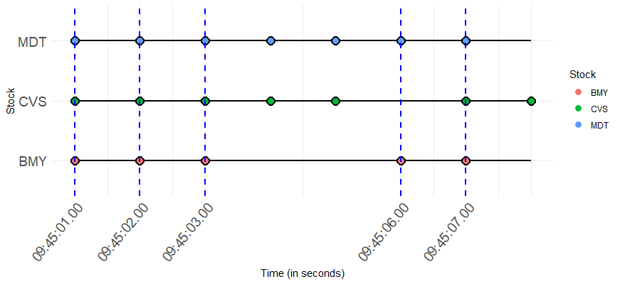
Why synchronization is necessary? In this section we describe refresh time sampling which allows synchronization of high frequency prices from multiple stocks. In high frequency trading (HFT) conducting multivariate analysis is difficult since assets do not trade on a fixed grid, trades and quotes don’t arrive synchronously. Hence synchronization of HFT data from multiple assets is necessary. As in Section (2.5.3), we briefly describe the refresh sampling procedure for synchronization of high frequency prices from multiple stocks.

Assume there are $p$ stocks, and trading time of the $i^{th}$ stock is given by $t_{i\ell}$, $\ell=1,\cdots,n_{i}$ , $i=1,\cdots,p$. For a given time $t$, define $N_{t}^{i}=$ the number of $t_{i\ell}\leq t$, $\ell=1,\cdots,n_{i}$, which counts the number of distinct data points $t_{i\ell}$ available for the $i^{th}$ asset up to time $t$. The first refresh time is defined as $\tau_{1}=\max\left\{t_{11},\ldots,t_{p1}\right\}$, which is the first time taken to trade all assets and refresh their posted prices. The subsequent refresh times are defined as follows. Given the $j^{th}$ refresh time $\tau_{j}$, define the $(j+1)^{th}$ refresh time

Suppose there are $m$ refresh time points $\tau_{1},\cdots,\tau_{m}$. Intuitively, $\tau_{2}$ is the second time when all the assets are traded and their prices are refreshed. In our empirical analysis we consider three health sector stocks BMY, CVS and MDT traded on NYSE on $24^{th}$ June, $2016$. We consider the high frequency prices for these three stocks and illustrate the refresh time sampling procedure for synchronization of multivariate analysis which we discuss later. Figure 1 illustrates the refresh time sampling idea and in this example we have $\tau_{1}=09:45:01.00$,$\tau_{2}=09:45:02.00$, $\tau_{3}=09:45:03.00$, $\tau_{4}=09:45:06.00$ and $\tau_{5}=09:45:07.00$ are the first five refresh times.

Let $\boldsymbol{r}_{t_{j}}=(r_{1t_{j}},r_{2t_{j}},\cdots,r_{pt_{j}})^{\prime}$, $j=1,\cdots,T$ be a $p$-dimensional vector of zero mean log returns of $p$ financial assets observed at irregularly spaced time points $t_{1},\cdots t_{T}$. Here, $t_{j}$ denotes the time of the $j^{th}$ observation, and $g_{j}=t_{j}-t_{j-1},j>1$ denotes the known gap time between consecutive observations. We introduce irregular multivariate stochastic volatility (IR-MSV) model as

where,

where $\phi_{i}$ is the persistence parameter constrained by $|\phi_{i}|<1$, $i=1,\cdots,p$, $\mu_{i}$ is the location parameter for each asset $i=1,\cdots,p$ and $\mathbf{R}$ is the correlation matrix of the observation errors. Following Nagaraja et al. 2011 and our discussion in the previous section, we observe that $\{h_{i,t_{j}}\}$ is a stationary process for each $i=1,\cdots,p$. Since the error correlation matrix $\mathbf{R}$ is assumed to remain constant over time, we refer to (17) as a constant correlation IR-MSV model.

In this section, we describe Bayesian analysis for fitting the IR-MSV model in (17) to irregularly spaced multiple financial time series. We show the likelihood, prior, posterior and also discuss the computational aspects using MCMC algorithms. The likelihood function is

where $\mathbf{\Sigma}_{\mathbf{r}}=\mathbf{H}_{t_{j}}^{1/2}\mathbf{R}\mathbf{H}_{t_{j}}^{1/2}$ , $\boldsymbol{\sigma}=(\sigma_{1},\cdots,\sigma_{p})$ and $\boldsymbol{\phi}=(\phi_{1},\cdots,\phi_{p})$, and $\boldsymbol{\Theta}=(\boldsymbol{\sigma},\boldsymbol{\phi},\mathbf{R},\mu)$.

For $i=1,\cdots,p$, we assume the following priors:

where Lewandowski-Kurowicka-Joe (LKJ) distribution Lewandowski et al. 2009 is a useful prior for correlation matrices, and IG denotes the inverse gamma distribution.

The posterior distribution of $\boldsymbol{\Theta}$ is

where we have assumed independence of the priors and $\pi(\boldsymbol{h}_{t_{j}}|\boldsymbol{h}_{t_{j-1}},\boldsymbol{\sigma},\boldsymbol{\phi})$ is the joint distribution of the stochastic volatilities as in (18). We employ a block random walk sampler for the correlation matrix $\mathbf{R}$ and for other parameters i.e. $(\boldsymbol{\sigma},\boldsymbol{\phi},\mu)$ we employ a Metropolis-Hastings adaptive random-walk sampler with a univariate normal proposal distribution, which are the default samplers in NIMBLE package (de Valpine et al. 2017) in R.

In this simulation our goal is to examine the effect of the correlation among the components on the accuracy of estimation. We generated 100 sets of zero mean log returns data from the IR-MSV model represented by equations (17) and (18) with $p=3$ and $T=5000$. The gap times $g_{j},1\leq j\leq T$ are generated using a similar procedure as described in Section 2.3. The $3\times 3$ correlation matrix has the following representation

We describe three different scenarios. In scenario 1, we consider moderate positive correlations among the components with $\rho_{12}=0.6$, $\rho_{13}=0.4$ and $\rho_{23}=0.2$. In scenario 2, we consider a mix of high and low positive correlation and a negative correlation with $\rho_{12}=-0.4$, $\rho_{13}=0.7$ and $\rho_{23}=0.3$. In scenario 3, we consider all correlations to be equal, high and positive with $\rho_{12}=\rho_{13}=\rho_{23}=0.7$.

We run 210000 MCMC iterations and discard the first 10000 as burn-in and thinned every $400^{th}$ sample to reduce autocorrelation between MCMC samples. We assessed the convergence for the parameters using trace and posterior density plots. In Table 4, Table 5, and Table 6 we report the posterior sample mean along with their true values and $95\%$ credible intervals averaged the 100 data sets for scenario 1, scenario 2 and scenario 3 respectively.

We considered the intra-day prices for MDT, BMY and CVS traded on June 24, 2016. We aggregated the high frequency prices at the one second level by taking the price with respect to the latest time point as in Buccheri et al. 2021b. There were 10066, 8797 and 11330 observations (transactions) for MDT, BMY, and CVS respectively. We synchronized these prices from three stocks using the refresh time sampling approach (Barndorff-Nielsen et al. 2011) to obtain a sample size of $T=6239$ synchronized observations. A brief description of refresh sampling technique is discussed in (Section 2.5.3). Using these irregularly spaced refreshed prices ($P_{t_{j}}$) we calculate the log returns as

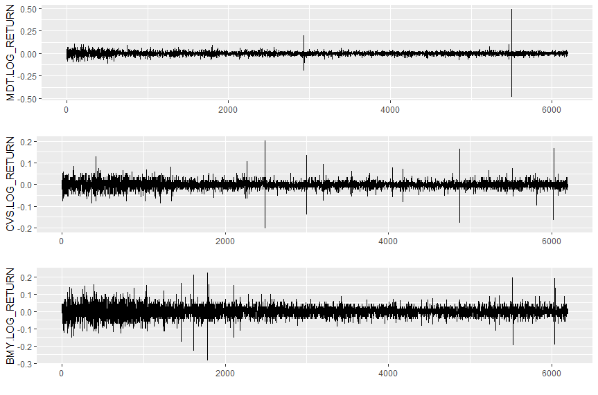
We have plotted the time series of log returns calculated from the refreshed prices of MDT, BMY and CVS on $24^{th}$ June, 2016 in Figure 2. They seem to be fairly correlated.

We fit IR-MSV model as in equations (17) and (18) to the irregularly spaced multivariate intraday log returns series of three stocks. We use first 6195 observations for fitting IR-MSV model and kept 44 observations as hold out samples. We have used exactly the same priors for the parameters as in the simulation setup. We run 300,000 MCMC iterations and discard the first 50,000 as burn-in to obtain samples from every $500^{th}$ iteration of the last 250,000 iterations. For convergence of MCMC iterations we have used trace and posterior density plots. In Table 7, we report the posterior sample mean along with their $95\%$ credible intervals.

All parameters lie within the $95\%$ credible intervals limits. The estimated correlations are moderate indicating fair dependency among the components which is expected. The persistence parameter for BMY is much higher than that of CVS and MDT indicating the temporal correlation of volatility of BMY is much higher than the temporal correlation of volatility of CVS and MDT.

We have also fitted IR-SV models to the univariate refreshed log return series of each stock of length $T=6195$. We have used the same prior as discussed in the simulation study of IR-SV models in Section 2.3. We run 550,000 MCMC iterations and discard the first 50,000 as burn-in to obtain samples from every 1000th iteration of the last 500,000 iterations. In Table 10, Table 8 and Table 9 we report the posterior sample mean along with their $95\%$ credible intervals. All the parameters lie inside the $95\%$ credible intervals. Convergence for the parameters are assessed using trace and posterior density plots. We observe that the persistence parameter $\phi$ for BMY is higher than that of CVS and MDT which is consistent with the result obtained in case of IR-MSV model fitting.

One of the early approaches to model the return series sampled at irregularly spaced time intervals set by the trade arrivals is ACD-GARCH model by Ghysels and Jasiak 1998. This is a random coefficient GARCH, or doubly stochastic GARCH, where the stochastic durations between transactions determine the parameter dynamics for the GARCH equation. They proposed a Generalized Method of Moments (GMM) based two-step procedure for estimating the parameters. ACD-GARCH is quite cumbersome to estimate and also difficult to generalize to multiple time series. Meddahi et al. 2006 proposed a GARCH type model for irregularly spaced data which is an exact discretization of continuous time stochastic volatility processes observed at irregularly spaced times. Their model combines the advantages of ACD-GARCH Ghysels and Jasiak 1998 and ACD (Engle and Russell 1998). A continuous version of GARCH (COGARCH) is another way to model irregularly spaced time series data (Maller et al. 2008). Recently, Buccheri et al. 2021a propose to model intraday log-prices through a multivariate local-level model with score-driven covariance matrices and to treat asynchronicity as a missing value problem.

In this section we do some preliminary investigation of extending the gap time autoregressive model of Nagaraja et al. 2011 to develop an irregular GARCH (IR-GARCH) model. We introduce the IR-GARCH model and discuss its properties. We conduct a small simulation study to assess the accuracy of estimation under different scenarios. Future research of this topic can be useful.

Let $\{r_{t_{j}}\}$ be a sequence of zero mean log-returns of an asset. Here $t_{j}$ denotes the time of the $j^{th}$ observation and $g_{j}=t_{j}-t_{j-1}$, $j>1$ is the known $j^{th}$ observed gap time. Suppose $\{\epsilon_{t_{j}}\}$ is a sequence of real valued independent and identically distributed random variables, having mean 0 and variance 1. We start with an IR-GARCH(1,1) model as shown below.

References

- Barndorff-Nielsen et al. (2011) O. E. Barndorff-Nielsen, P. R. Hansen, A. Lunde, and N. Shephard. Multivariate realised kernels: consistent positive semi-definite estimators of the covariation of equity prices with noise and non-synchronous trading. Journal of Econometrics, 162(2):149–169, 2011.
- Buccheri et al. (2021a) G. Buccheri, G. Bormetti, F. Corsi, and F. Lillo. A score-driven conditional correlation model for noisy and asynchronous data: An application to high-frequency covariance dynamics. Journal of Business & Economic Statistics, 39(4):920–936, 2021a.
- Buccheri et al. (2021b) G. Buccheri, F. Corsi, and S. Peluso. High-frequency lead-lag effects and cross-asset linkages: a multi-asset lagged adjustment model. Journal of Business & Economic Statistics, 39(3):605–621, 2021b.
- Chib et al. (2009) S. Chib, Y. Omori, and M. Asai. Multivariate stochastic volatility. In Handbook of financial time series, pages 365–400. Springer, 2009.
- de Valpine et al. (2017) P. de Valpine, D. Turek, C. J. Paciorek, C. Anderson-Bergman, D. T. Lang, and R. Bodik. Programming with models: writing statistical algorithms for general model structures with nimble. Journal of Computational and Graphical Statistics, 26(2):403–413, 2017.
- Engle and Russell (1998) R. F. Engle and J. R. Russell. Autoregressive Conditional Duration: A New Model for Irregularly Spaced Transaction Data. Econometrica, 66(5):1127–1162, 1998.
- Ghysels and Jasiak (1998) E. Ghysels and J. Jasiak. Garch for irregularly spaced financial data: the acd-garch model. Studies in Nonlinear Dynamics & Econometrics, 2(4), 1998.
- Lewandowski et al. (2009) D. Lewandowski, D. Kurowicka, and H. Joe. Generating random correlation matrices based on vines and extended onion method. Journal of multivariate analysis, 100(9):1989–2001, 2009.
- Maller et al. (2008) R. A. Maller, G. Müller, and A. Szimayer. Garch modelling in continuous time for irregularly spaced time series data. Bernoulli, 14(2):519–542, 2008.
- Meddahi et al. (2006) N. Meddahi, E. Renault, and B. Werker. Garch and irregularly spaced data. Economics Letters, 90(2):200–204, 2006.
- Nagaraja et al. (2011) C. H. Nagaraja, L. D. Brown, and L. H. Zhao. An autoregressive approach to house price modeling. The Annals of Applied Statistics, pages 124–149, 2011.
- Tsay (2005) R. S. Tsay. Analysis of financial time series. John wiley & sons, 2005.