Statistical post-processing of visibility ensemble forecasts
Abstract
To be able to produce accurate and reliable predictions of visibility has crucial importance in aviation meteorology, as well as in water- and road transportation. Nowadays, several meteorological services provide ensemble forecasts of visibility; however, the skill, and reliability of visibility predictions are far reduced compared to other variables, such as temperature or wind speed. Hence, some form of calibration is strongly advised, which usually means estimation of the predictive distribution of the weather quantity at hand either by parametric or non-parametric approaches, including also machine learning-based techniques. As visibility observations – according to the suggestion of the World Meteorological Organization – are usually reported in discrete values, the predictive distribution for this particular variable is a discrete probability law, hence calibration can be reduced to a classification problem. Based on visibility ensemble forecasts of the European Centre for Medium-Range Weather Forecasts covering two slightly overlapping domains in Central and Western Europe and two different time periods, we investigate the predictive performance of locally, semi-locally and regionally trained proportional odds logistic regression (POLR) and multilayer perceptron (MLP) neural network classifiers. We show that while climatological forecasts outperform the raw ensemble by a wide margin, post-processing results in further substantial improvement in forecast skill and in general, POLR models are superior to their MLP counterparts.
Keywords: classification, ensemble calibration, multilayer perceptron, proportional odds logistic regression, visibility
1 Introduction
According to the definition of the World Meteorological Organization (WMO), visibility “is the greatest distance at which a black object of suitable dimensions (located on the ground) can be seen and recognized when observed against the horizon sky” (WMO, 1992). This weather quantity plays a crucial role in aviation in all phases of flight and restricted visibility also makes both ship navigation and road transportation difficult. Hence, accurate and reliable visibility forecasts result in a direct economic benefit.
In general, weather forecasts are generated using numerical weather prediction (NWP) models, which are often run several times with varying model physics and/or initial conditions resulting in a probabilistic forecast represented by an ensemble of predictions (Bauer et al., 2015; Buizza, 2018a). With the help of a forecast ensemble, besides providing point forecasts for a given location, time point, and forecast horizon, one can also assess forecast uncertainty and estimate probability distributions of future weather variables (Gneiting and Raftery, 2005). However, in contrast e.g. to temperature, wind speed, or precipitation accumulation, most NWPs do not explicitly model visibility, so visibility forecasts must be derived from predictions of related quantities such as relative humidity or precipitation (Chmielecki and Raftery, 2011). Even nowadays only a few weather centres issue visibility ensemble forecasts. Examples include the multimodel Short-Range Ensemble Forecast System of the National Centers for Environmental Prediction covering the Continental US, Alaska, and Hawaii regions (Zhou et al., 2009) or the Ensemble Prediction System (EPS) of the European Centre for Medium-Range Forecasts (Molteni et al., 1996; ECMWF Directorate, 2012, ECMWF;), where visibility is part of the Integrated Forecasting System (IFS) since 2015 (ECMWF, 2021).
Despite the continuous improvement of the various operational EPSs over the past decades, ensemble forecasts still might display systematic bias or suffer from lack of calibration (Buizza et al., 2005, see e.g.), that calls for some form of post-processing (Buizza, 2018b). Moreover, visibility forecasts are even more problematic, as their predictive performance, similar to total cloud cover (Haiden et al., 2021), is highly below the skill of ensemble forecast of e.g temperature, wind speed, pressure or precipitation accumulation (Zhou et al., 2012, see e.g.).
Nowadays, one can select from a large collection of post-processing methods developed for a wide variety of weather variables; for an overview of the state-ot-the-art techniques see e.g. Wilks, 2018 or Vannitsem et al., 2021. Parametric approaches like non-homogeneous regression (Gneiting et al., 2005) or Bayesian model averaging (Raftery et al., 2005) provide full predictive distribution of the investigated weather quantity, whereas quantile regression-based approaches (Friederichs and Hense, 2007; Bremnes, 2019, see e.g.) result in probabilistic forecasts by estimating the quantiles of the forecast distribution. Moreover, in the last few years machine learning techniques such as quantile regression forests (Taillardat et al., 2016), distributional regression network (Rasp and Lerch, 2018), Berstein quantile network (Bremnes, 2020), or the classification and interpolation-based approach of Scheuerer et al., 2020 gain more and more popularity; for a recent comparison of neural network-based approaches we refer to Schultz and Lerch, 2022.
While visibility forecasts can be considered as continuous (e.g. ECMWF ensemble forecasts are provided in 1 m steps), most synoptic observation (SYNOP) stations report observations according to the WMO suggestions, that is “100 to 5 000 m in steps of 100 m, 6 to 30 km in steps of 1 km, and 35 to 70 km in steps of 5 km” (WMO, 2018, Section 9.1.2), and observed visibility is rounded down to the nearest reported value. In this way, one has just 84 different values, so the corresponding predictive distribution is a discrete probability law. Hence, post-processing of visibility forecasts can be considered as an 84-group classification problem resulting in the probabilities of the different reported values. The situation is similar to the case of total cloud cover (TCC) reported in eighths of the sky covered by clouds called oktas taking just nine different values, only in this case the number of classes is almost ten times larger. To calibrate TCC ensemble forecasts, Hemri et al., 2016 proposed multiclass logistic regression (Izenman, 2008, MLR;) and proportional odds (or ordered) logistic regression (McCullagh, 1980, POLR;), whereas Baran et al., 2021 investigated the forecast skill of several machine learning-based classification methods such as multilayer perceptron neural network (Goodfellow et al., 2016, MLP;), gradient boosting machine (Friedman, 2001) and random forest algorithms (Breiman, 2001).
In the present work we investigate the predictive performance of POLR and MLP approaches to calibration of ECMWF visibility ensemble forecasts, as these two methods exhibit the best forecast skill among the techniques investigated by Baran et al., 2021 in the context of post-processing ensemble predictions of TCC. As reference forecasts, we consider the raw visibility ensemble and climatology.
The paper is organized as follows. After a brief description of the studied visibility datasets in Section 2, we review the POLR and MLP methods in Section 3 and also provide the investigated approaches to training data selection and the considered verification tools. Results of our two case studies are reported in Section 4, followed by short discussion and conclusions in Section 5.
2 Data
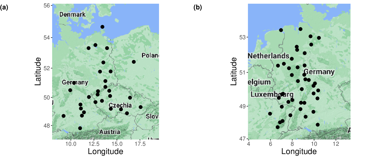
We consider two datasets consisting of ECMWF visibility ensemble forecasts and corresponding validating observations covering different time periods but having slightly overlapping ensemble domains. As mentioned, observations are reported according to the WMO suggestions in values
whereas the matching of forecasts (given in 1 m steps) and observations is performed by rounding down to the closest reported value.
In the case of the first dataset, as predictions we have the operational 51-member ECMWF visibility ensemble forecasts (control forecast (CTRL) and 50 members (ENS) generated using random perturbations) for calendar years 2020 and 2021 for 30 SYNOP stations in Germany, Czech Republic, and Poland (Figure 1a). All forecasts are initialized at 0000 UTC and we consider 40 different lead times from 6 h to 240 h with a time step of 6 h. This data set is fairly complete as there are no missing observations at all and one has just two days when some predictions are missing; namely, there are no exchangeable ensemble members with forecast horizon 132 h initialized 2 June 2021 and 114 h initialized 17 December 2021.
We also investigate visibility data from the EUPPBench benchmark dataset (Demaeyer at al., 2023), where besides the 51-member operational ECMWF ensemble the high-resolution (HRES) forecast is also available. The studied dataset consists of ensemble forecasts for calendar years 2017 – 2018 initialized at 0000 UTC with a forecast horizon of 120 h and temporal resolution of 6 h for 42 SYNOP stations in Germany and France (Figure 1b). Here around 1.5 % of the forecast cases is incomplete due to missing station observations.
3 Post-processing methods and verification tools
Following the notations of Baran et al., 2021, denote by the observed visibility for a given location and time point with defined in Section 2, and let be the corresponding ensemble forecast with a given forecast horizon, where denotes the high-resolution forecast, is the control run and correspond to the 50 exchangeable members . As is a discrete random variable, the predictive distribution of is specified by conditional probabilities with respect to the ensemble forecast
| (3.1) |
Naturally, instead of the raw forecast , in (3.1) the conditional probability can be taken with respect to any feature vector derived from the ensemble and/or other covariates such as forecasts of additional weather quantities or station specific information like location, altitude or land use.
3.1 Proportional odds logistic regression
As mentioned in the Introduction, in the case of discrete weather quantities post-processing is reduced to a classification problem, where MLR is a frequently used and powerful tool. However, given an -dimensional feature vector , an MLR model for an 84-group classification has free parameters to be estimated from the training data. Hence, to avoid numerical issues in the estimation process, one requires an extremely large training data set consisting of past forecast-observation pairs.
A more parsimonious approach is the POLR model designed to fit ordered data, like the visibility observations at hand. In this case the conditional cumulative distribution of with respect to an -dimensional feature vector is given as
| (3.2) |
where and we assume , so the POLR model has unknown parameters.
3.2 Multilayer perceptron neural network
For both continuous and discrete weather quantities, the application of neural networks has increased in popularity for calibration. For the latter, instead of a parametric approach, one can use a classical feedforward multilayer perceptron (MLP) neural network for classification. A classical MLP consists of multiple layers and neurons or nodes, each of which is a transformed (by an activation function) weighted sum of the node values from the previous layer plus an additional bias term. The features are ”fed” to the input layer, and the predictions of the distribution of the various classes are made on the output layer. The number of hidden layers and neurons in them are tuning parameters of the network and provide the level of abstraction. For additional information, we refer to Goodfellow et al., 2016.
3.3 Training data selection
Both parameters of the POLR model and weights of the MLP neural network are estimated with the help of training data, and the spatial and temporal composition of this set of forecast-observation pairs is a key issue in statistical post-processing. The basic approaches to spatial selection are local and regional (global) modelling (Thorarinsdottir and Gneiting, 2010). In the local case only past data of the station of interest are used to obtain the predictive distribution resulting in distinct POLR model parameters and MLP networks for the different stations. Provided one has a long enough training period to avoid numerical issues (Hemri et al., 2014, for optimal training period lengths for different weather quantities see e.g.), local models usually outperform their regional counterparts, which pool training data of the whole ensemble domain and all stations share the same set of POLR model parameters and a single MLP network. Regional modelling can be performed with the help of rather short training periods; however, this approach is not really suitable for large and heterogeneous domains. As a bridge between these two traditional spatial selection methods, Lerch and Baran, 2017 propose a semi-local approach, where first clusters of stations with similar characteristics are formed using -means clustering, then within each cluster a regional estimation is performed.
Concerning the temporal selection, a popular approach is the use of rolling training periods, where models are trained with the help of ensemble forecasts and validating observations from the preceding calendar days. This method enables models to quickly adapt e.g. to seasonal changes; however, in many situations the use of large fixed training data sets (Rasp and Lerch, 2018; Ghazvinian et al., 2021, see e.g.) or yearly training considering data of the last couple of years before the year of the given date (Hemri et al., 2016; Baran et al., 2021, see e.g.) might also be beneficial.
3.4 Verification scores
As proposed by Gneiting et al., 2007, the evaluation of the predictive performance of probabilistic forecasts should be based on the idea of “maximizing the sharpness of the predictive distributions subject to calibration”. Calibration means a statistical consistency between forecasts and observations, while sharpness refers to the concentration of the predictive distribution.
A simple graphical tool for assessing calibration is the probability integral transform (PIT) histogram (Wilks, 2019, Section 9.5.4). The PIT is defined as the value of the predictive cumulative distribution function (CDF) evaluated at the verifying observation, where for non-continuous laws randomization should be applied at points of discontinuity (Gneiting and Ranjan, 2013). For a properly calibrated probabilistic forecast the PIT follows a standard uniform distribution; moreover, the shape of the PIT histogram can provide hints to the possible reason for the lack of calibration.
The sharpness of a probabilistic forecast can be investigated by examining the widths of various prediction intervals. In the case studies of Section 4, similar to Hemri et al., 2016, we compare the competing forecasts in terms of the average width of the centered 90 % prediction interval. Furthermore, one can also calculate the coverage of this interval defined as the proportion of validating observations located between the lower and upper 5 % quantiles of the predictive distribution. The deviation in coverage from the confidence level can serve as a measure of calibration.
Calibration and sharpness can also be assessed simultaneously by using proper scoring rules, which are loss functions assigning numerical values to forecast-observation pairs . Here we consider the continuous ranked probability score (CRPS; Wilks, 2019, Section 9.5.1) and the logarithmic score (Good, 1952, LogS;), being the most popular scoring rules in atmospheric sciences. Note, that in the case of visibility reported according to WMO suggestions (see Section 2), a forecast is characterized by a probability mass function (PMF) specifying a discrete probability distribution on . Hence, the CRPS equals
| (3.3) |
whereas the LogS is defined as
that is as the negative logarithm of the PMF at the observation. Both CRPS and LogS are negatively oriented (the smaller the better), and expression (3.3) is the discrete form of the representation of the CRPS
provided by Gneiting and Raftery, 2007, where and are independent random variables with distribution and finite first moment.
For each of the investigated forecast horizons, the predictive performance of various probabilistic forecasts is quantified by the mean CRPS () and mean LogS () over all forecast cases in the verification data. Furthermore, one can obtain a deeper insight into the smaller differences in forecast skill of the compering predictions by examining continuous ranked probability skill scores (CRPSS) and logarithmic skill scores (LogSS), which measure the improvement in terms of CRPS and LogS of a forecast with respect to a reference forecast , respectively (Murphy, 1973; Gneiting and Raftery, 2007, see e.g.). CRPSS and LogSS are defined as
where and denote the mean score values corresponding to forecasts and , respectively. Note that skill scores are positively oriented, so larger values mean better predictive performance.
Furthermore, as point forecasts, we consider the ensemble mean and the means of the predictive distributions of the competing forecasts, which are evaluated with the help of the corresponding root mean squared errors (RMSEs).
Finally, the uncertainty of the verification scores and statistical significance of the score differences are addressed by providing confidence intervals for the skill scores. The standard deviations required for the confidence bounds are calculated from 2000 block bootstrap samples obtained using the stationary bootstrap scheme, where the mean block length is computed according to Politis and Romano, 1994.
4 Results
In the case studies of Sections 4.2 and 4.3, the forecast skill of the POLR and MLP approaches described in Sections 3.1 and 3.2, respectively, are evaluated. Both methods require training data, which should be large enough to allow reliable modelling. We consider 350-day rolling training periods, which in the case of regional estimation means 10500 forecast cases for the first dataset and 14700 forecast cases for the second one for each training step. In what follows, regional POLR and MLP models are referred to as POLR-R and MLP-R, respectively. We also investigate clustering-based semi-local modelling, where the clusters of stations are derived using -means clustering of feature vectors depending on station climatology over the training period. In particular, each station is represented by a three-dimensional feature vector providing the frequencies of visibility intervals 0 to 5000 m, 5000 to 30000 m and 30000 to 70000 m. With the shift of the training data the clusters are recalculated dynamically and in general, 4 clusters are formed in the case of forecasts for 2020 – 2021 and 8 in the case of the EUPPBench data, provided each cluster contains at least 4 locations. Otherwise, the number of clusters is reduced and the clustering-based estimation might even fall back to regional modelling. For the semi-local POLR and MLP approaches notations POLR-C and MLP-C are used and note that the above feature vectors and the applied number of clusters are based on a preliminary analysis of the climatology of each station. Finally, local training is also investigated, the corresponding models are denoted as POLR-L and MLP-L.
In both case studies the forecast skill of the competing post-processing methods is tested on data for a complete calendar year. As reference forecasts we consider the raw ECMWF visibility ensemble and climatology, where observations of a rolling training period of a given length are considered as a forecast ensemble.
Before calculating the input features of the POLR and MLP models, a normalization of the forecasts is performed; namely, all forecast values are divided by 70000. Then we consider the following set of predictors: the (normalized) control member of the ensemble , the mean of the 50 (normalized) exchangeable members, the variance of the 51-member (normalized) operational ensemble, in the case of the EUPPBench dataset the (normalized) high-resolution forecast , and the proportions and of ensemble members predicting visibility up to 1000 m, 1000 to 2000 m and more than 30000 m, respectively. Note that normalization is required to have all input features commensurate. Finally, following the suggestions of e.g. Dabering et al., 2017, seasonal variations are addressed by adding annual base functions
to the input features, where denotes the day of the year.
4.1 Implementation details
POLR models are fit using the R package MASS (Venables and Ripley, 2002), while MLP classification is based on the package RSNNS making the Stuttgart Neural Network Simulator (Zell et al., 1994) available in R. The neural network has two hidden layers with 25 – 25 neurons, the maximal number of iterations to learn is restricted to 200, the learning rate is and both hidden layers use the logistic activation function.
To handle numerical problems with LogS calculation caused by zero predicted probabilities, we follow the procedure applied by Hemri et al., 2016 and Baran et al., 2021. Extremely low values of the PMF are replaced with a probability , which ensures that the corresponding reported visibility at the given observation hour appears at least once a year with probability . This means that for an observation instead of we consider , where , and normalize the obtained values to get a PMF again. For this approach results in .
4.2 Calibration of 51-member visibility ensemble forecasts

| MLP-L | MLP-C | MLP-R | POLR-L | POLR-C | POLR-R | Climatology | |
|---|---|---|---|---|---|---|---|
| CRPS | 70.65 % | 70.75 % | 72.94 % | 68.09 % | 69.60 % | 72.52 % | 75.60 % |
| LogS | 45.31 % | 44.10 % | 44.88 % | 44.28 % | 43.45 % | 44.44 % | 66.05 % |
We study post-processing of visibility ensemble forecasts with the help of locally, semi-locally and regionally trained POLR and MLP models based on the 8-dimensional feature vector . Following the suggestions of Hemri et al., 2016, for the POLR models the weights of , and are kept non-negative by excluding iteratively covariates with negative coefficients. The predictive performance of the competing post-processing methods is tested on data for the calendar year 2021. In the case of the reference climatological forecasts we consider a 30-day rolling training period, which value is chosen by the comparison of the overall mean CRPS, RMSE of mean forecasts and coverage of 90 % central prediction intervals for training periods of length 25, 30, …, 50 and 350 days.


According to Figure 2a, in terms of the mean CRPS all post-processing methods outperform the raw ECMWF ensemble forecast for all forecast horizons by a wide margin and climatology also performs rather well. The clear diurnal cycle in the mean CRPS corresponds to the different observation times (0000, 0600, 1200 and 1800 UTC). Note that the superiority of climatology over the raw visibility forecasts is fully in line with the results of Chmielecki and Raftery, 2011. A deeper insight into the differences between the various calibration techniques can be obtained from Figure 2b depicting the CRPSS values with respect to climatology. In general, clustering-based modelling is superior to regional, and the advantage of post-processing with respect to climatology decreases with the increase of the lead time. For POLR models the chosen training period length is long enough even for reliable local estimation and the POLR-L approach results in the highest skill score for all lead times. This is not the case for the MLP models, where the CRPSS of the semi-locally estimated MLP-C is often above the skill score of the MLP-L, especially for lead times corresponding to 0600 UTC. POLR models outperform their MLP counterparts for most of the forecast horizons; however, up to 156 h even the poorest MPL-R has better skill than climatology. A possible ranking of the competing methods can be obtained from Table 1 giving the overall mean score values of calibrated and climatological forecasts as proportions of the corresponding mean score of the raw ECMWF ensemble. POLR-L results in the lowest mean CRPS, closely followed by POLR-C.
As Figure 3a and Table 1 show, the difference between raw and post-processed forecasts in terms of the mean LogS is even more pronounced than in terms of the mean CRPS; however, the general picture slightly changes. On the one hand, all post-processing methods outperform climatology by a wide margin. On the other hand, in terms of the LogS, clustering-based modelling is clearly superior to local estimation. According to Figure 3b, for most of the forecast horizons MLP-L underperforms even MLP-R, and at lead times corresponding to 0600 and 1200 UTC, POLR-R also results in positive LogSS with respect to POLR-L.
To enlighten the uncertainty of the investigated verification scores and statistical significance of the score differences, in Figure 4 the CRPSS and LogSS values of some post-processing approaches are accompanied with 95 % confidence intervals. According to Figure 4a, the advantage of the best-performing POLR-L model over climatology in terms of the mean CRPS is clearly significant for all lead times but 204 h and 228 h. Regarding the LogS (Figure 4b), POLR-L significantly outperforms MLP-L for all lead times, whereas the difference between POLR-L and the best performing POLR-C is significant at a 5 % level only at forecast horizons corresponding to 0600 UTC.
| MLP-L | MLP-C | MLP-R | POLR-L | POLR-C | POLR-R |
|---|---|---|---|---|---|
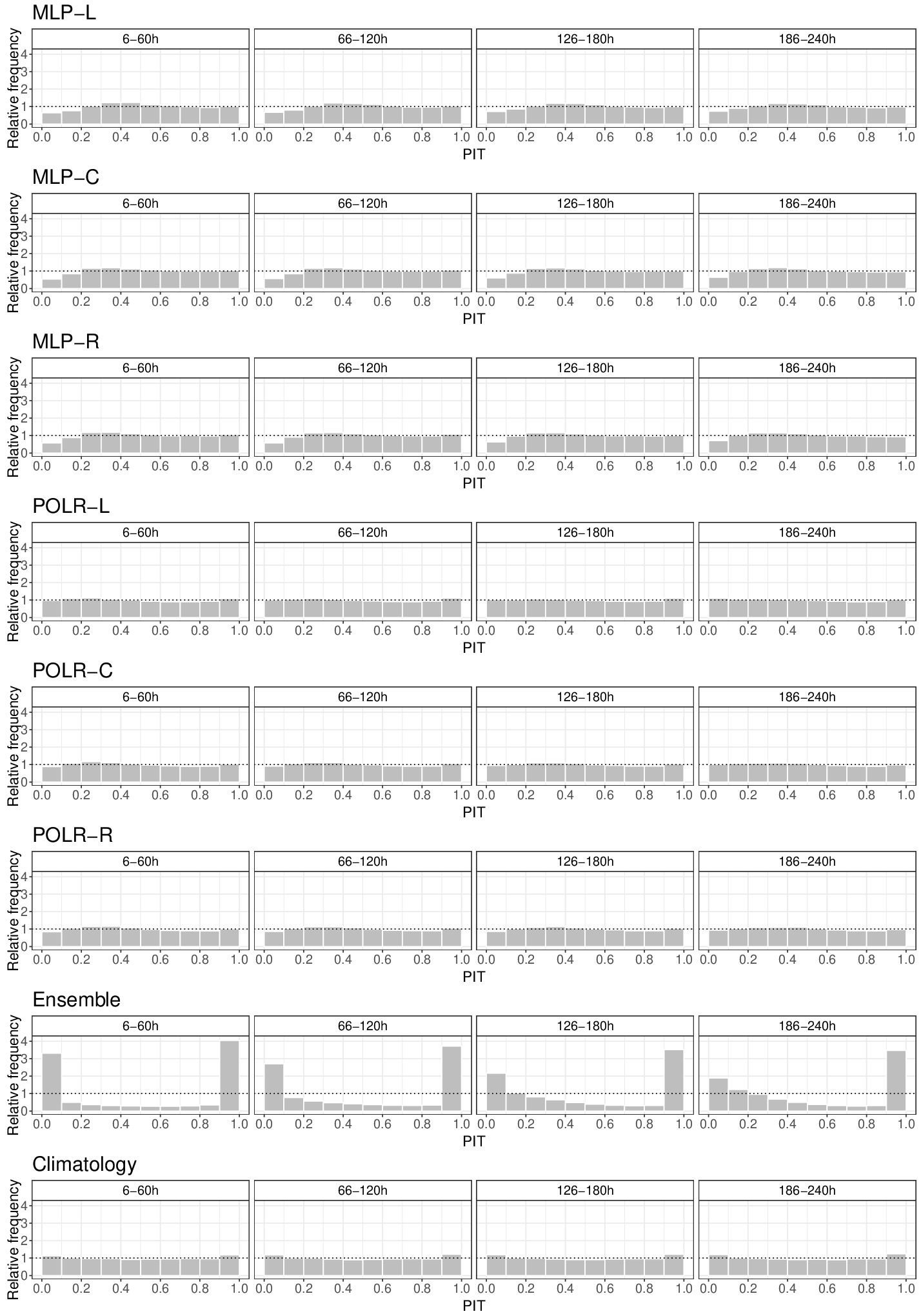
Furthermore, PIT histograms of Figure 5 also demonstrate the positive effect of post-processing and the superiority of climatology over the raw visibility ensemble forecasts. The histograms of the latter are rather U-shaped with a more and more pronounced bias with the increase of the forecast horizon. All other forecasts result in PIT values that are much closer to the desired standard uniform distribution; however, climatology still exhibits a small underdispersion, whereas MLP post-processed predictions are slightly overdispersive. For all calibrated forecasts the moment-based test (Knüppel, 2015) rejects uniformity at a 5 % level of significance for all 40 investigates lead times. Nevertheless, a possible ranking of the competing post-processing approaches in terms of goodness of fit of PIT can be obtained from Table 2 reporting the mean -values of the tests over all considered lead times (the larger the better). Note that for raw and climatological forecasts the PIT values are concentrated around 52 and 31 bins (ensemble size + 1), respectively. Hence, these PIT histograms fall back to the corresponding verification rank histograms (Wilks, 2019, Section 9.7.1).

The improved calibration of post-processed and climatological forecasts can also be observed in Figure 6a showing the coverage of 90 % central prediction intervals. For the raw forecasts this coverage ranges from 28 % to 66 % and shows an increasing trend with a clear diurnal cycle. For post-processed and climatological forecasts the diurnal cycle is far less pronounced and one cannot observe dependence on the forecast horizon. The coverage of climatology is almost perfect, whereas post-processed forecasts result in coverages slightly above 90 %. For the POLR models the mean absolute deviations over all lead times from the desired 90 % are 2.53 % (POLR-L), 2.96 % (POLR-C) and 2.99 % (POLR-R), while for the MLP approaches one gets 4.86 % (MLP-R), 4.98 % (MLP-C) and 4.52 % (MLP-R). Note that for climatological forecasts this mean absolute deviation is just 0.69 %. Naturally, the price for the better calibration of post-processed and climatological forecasts has to be paid in the loss of the sharpness. As depicted in Figure 6b, the raw ECMWF visibility ensemble results in far the narrowest 90 % central prediction intervals and in general, the average width values of the different forecasts are fairly consistent with the corresponding coverages.

Finally, according to Figure 7a, compared with the raw ensemble all POLR and MLP models substantially improve the accuracy of the mean forecast, whereas the advantage of climatology is far less pronounced, especially for shorter forecast horizons. Note that the ranking of the different forecasts with respect to the RMSE of the mean (Figure 7b) is completely in line with the ordering based on the mean CRPS (Figure 2b), and the POLR-L approach again outperforms the competitors for all lead times.
Besides the 30-day reference climatology, the predictive performance of climatological forecasts based on a 350-day rolling training period was also tested. However, such a long training period is unlikely to capture the seasonal variations in visibility. In terms of the mean CRPS and RMSE of the mean, this forecast is far behind the various MLP and POLR models, its mean absolute deviation in 90 % coverage from the required value is 3.90 %, combined with an average width similar to the MLP approaches. The only score where the performance of the 350-day climatology is reasonable is the LogS, at 192 h, 216 h and 240 h it can compete with the regional versions of both studied post-processing techniques.
4.3 Calibration of EUPPBench visibility ensemble forecasts

| MLP-L | MLP-C | MLP-R | POLR-L | POLR-C | POLR-R | Climatology | |
|---|---|---|---|---|---|---|---|
| CRPS | 66.35 % | 65.53 % | 68.47 % | 64.67 % | 66.05 % | 69.96 % | 68.19 % |
| LogS | 45.48 % | 43.91 % | 44.45 % | 44.86 % | 43.66 % | 44.55 % | 64.39 % |
As mentioned, in post-processing of the 52-member EUPPBench benchmark visibility forecasts as an additional predictor we consider the normalized high-resolution forecast and investigate the performance of POLR and MLP models with an extended feature vector
Similar to the previous case study, for the local, semi-local and regional POLR models the coefficients of and are forced to be non-negative. Furthermore, the performance of the various forecasts is compared using forecast-observation pairs for the calendar year 2018 and following the same selection procedure as in Section 4.2, for the reference climatology now a 40-day training period is chosen. Finally, we tested again the skill of those climatological forecasts, that are based on the same 350-day training period as the post-processing approaches.

In line with the case study of Section 4.2, both climatological and post-processed forecasts (MLP and POLR models) result in far lower mean CRPS values than the raw EUPPBench ensemble for all lead times (see Figure 8a); however, now the ranking of the competing predictions is different. As depicted in Figure 8b, climatology performs surprisingly well, clearly outperformed for all forecast horizons only by the locally trained POLR and MLP approaches. Except for lead times corresponding to 1200 UTC, POLR-C and MLP-C also yield positive CRPSS with respect to climatology and are superior to MLP-L, whereas POLR-R and MLP-R follow a similar pattern but perform much worse than the corresponding semi-local models. The ranking of forecasts based on Figure 8b (POLR-L – MLP-C – POLR-C – MLP-L – Climatology – MLP-R – POLR-R) is also confirmed by Table 3 reporting the overall improvement in mean scores with respect to the raw EUPPBench visibility ensemble forecasts.

In terms of the mean LogS, climatology is again far behind post-processed forecasts; Figure 9a is rather similar to Figure 3a. According to Figure 9b, semi-local models clearly outperform their local counterparts and except for lead times corresponding to 1200 UTC, even the regional approaches are superior to the local ones. From the studied calibration methods POLR-C results in the lowest mean LogS, closely followed by the MLP-C, whereas MLP-L shows the poorest performance, see also Table 3.
The good performance of climatology with regard to the mean CRPS is also confirmed by Figure 10a, as at forecast horizons 36 h, 60 h, 66 h, 84 h, 90 h, 108 h and 114 h even the best performing POLR-L model fails to result in significantly positive CRPSS at a 5 % level. Furthermore, in contrast to the case study of Section 4.2, the LogSS of POLR-C with respect to POLR-L is significantly positive for all investigated lead times, whereas the 95 % upper bound for the LogSS of the least performing MLP-L almost coincides with the reference line. This means a barely significant difference between the MLP-L approach and POLR-L.
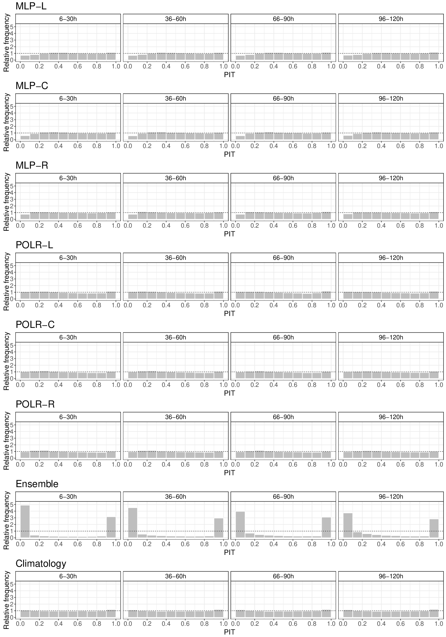
The PIT histograms of Figure 11 tell us the same story about calibration as the corresponding panels of Figure 5. Raw EUPPBench forecasts are highly underdispersive with a small bias increasing with the forecast horizon, whereas climatology and all post-processing approaches display rather flat histograms. The test again reject uniformity for all calibrated forecasts for all lead times; however, now the two regional approaches results in the highest overall mean -values, see Table 4.
According to Figure 12a, with the increase of the forecast horizon the coverage of 90 % central prediction intervals of the raw EUPPBench forecasts increases from 22 % to 51 %, and shows again a clear diurnal cycle. This diurnal cycle is also preserved in the coverage values of climatological and post-processed forecasts; however, these curves do not display any further dependence on the forecast horizon and are just slightly above 90 %. Similar to Figure 6a, the best coverage again corresponds to climatological forecasts with a mean absolute deviation from the nominal value of 0.82 %, followed by the POLR models (POLR-L: 1.32 %; POLR-C: 2.12 %; POLR-R: 3.03 %) and MLP approaches (MLP-L: 3.69 %; MLP-C: 4.59 %; MLP-R: 4.35 %). Again, the average widths of 90 % central prediction intervals depicted in Figure 12b are nicely in line with the corresponding coverage values, with the POLR-L approach providing the sharpest post-processed forecasts.
Furthermore, in line with the case study of Section 4.2, all post-processing methods result in a considerable decrease in the RMSE of the mean forecast (see Figure 13a). Moreover, according to Figure 13b, for the EUPPBench data climatology is fully able to catch up with the POLR and MLP models and for forecast horizons corresponding to 1200 UTC it definitely outperforms their local versions.
| MLP-L | MLP-C | MLP-R | POLR-L | POLR-C | POLR-R |
|---|---|---|---|---|---|

Finally, 350-day climatology performs well again only in terms of the LogS; however, in this case it is still slightly behind the post-processed forecasts for all forecast horizons.

5 Conclusions
We investigate the predictive performance of the proportional odds logistic regression and multilayer perceptron neural network classifiers for statistical post-processing of visibility ensemble forecasts in the situation, when observations are reported in discrete values following the suggestions of the World Meteorological Organization. In two case studies, the forecast skill of the proposed calibration methods is tested on two different datasets of ECMWF visibility ensemble forecasts covering two overlapping geographical regions and two different time domains. First, we consider the 51-member operational forecasts for 30 locations in Central Europe with a forecast horizon of 240 h and a time step of 6 h for calendar years 2020 and 2021. The second dataset is part of the EUPPBench benchmark data, where the ECMWF high-resolution forecast is also included. It contains ensemble forecasts and validating observations for 42 stations in Germany and France for calendar years 2017 – 2018 with a maximal lead time of 120 h and temporal resolution of 6 h. Local, semi-local, and regional training is tested for both post-processing approaches, which are based on 350-day rolling training periods. As reference, we consider raw and climatological visibility forecasts where for the latter short rolling past time intervals are chosen in order to capture seasonal variations in visibility observations.
In general, climatological and post-processed forecasts outperform the raw ensemble in terms of the mean CRPS, the mean LogS, and the RMSE of the mean forecast over the verification data by a wide margin, but the difference decreases with the increase of the forecast horizon. They result in better coverage but wider central prediction intervals than the raw ECMWF visibility forecasts and the corresponding PIT histograms are much closer to the uniform distribution than those of the raw ensemble. POLR models are superior to their MLP counterparts which is in line with the findings of Baran et al., 2021 in the case of total cloud cover forecasts, and the performance of climatology is comparable with the skill of post-processed forecasts in all investigated scores but the mean LogS. From the competing post-processing methods the locally trained POLR model shows the best overall performance, whereas for the machine learning-based approaches the semi-local training is often superior to the local one.
The results of the current work open several avenues for future research. First, here as inputs of our post-processing models, we have used only features derived from the raw visibility forecasts. However, as recent studies demonstrate (Rasp and Lerch, 2018; Baran et al., 2021; Schultz and Lerch, 2022, see e.g.), the incorporation of additional predictors, especially in the case of machine learning-based approaches, where the extension of the input feature set is rather straightforward, might significantly improve the forecast skill. Furthermore, so far we have focused on univariate forecasts for a single location and forecast horizon. However, in the last decade, a wide range of multivariate post-processing techniques have been developed, which are able to restore dependence structures lost during the univariate calibration, for an overview see e.g. Lerch et al., 2020 or Lakatos et al., 2023. The investigation of spatially and/or temporally consistent calibrated visibility forecasts might be an other interesting direction of our future work. Finally, as several SYNOP stations report visibility in 10 m steps which can be considered almost as continuous, using e.g. the interpolation technique of Scheuerer et al., 2020, one might try to develop methods for estimating continuous predictive distributions for this weather quantity.
Acknowledgments. The authors gratefully acknowledge the support of the the ÚNKP-22-3 New National Excellence Program of The Ministry for Innovation and Technology and of the National Research, Development and Innovation Office under Grant No. K142849. Finally, they are indebted to Zied Ben Bouallègue for providing the ECMWF visibility data.
References
- Baran et al., (2021) Baran, Á., Lerch, S., El Ayari, M. and Baran, S. (2021) Machine learning for total cloud cover prediction. Neural. Comput. Appl. 33, 2605–2620.
- Bauer et al., (2015) Bauer, P., Thorpe, A. and Brunet, G. (2015) The quiet revolution of numerical weather prediction. Nature 525, 47–55.
- Breiman, (2001) Breiman, L. (2001) Random forests. Mach. Learn. 45, 5–32.
- Bremnes, (2019) Bremnes, J. B. (2019) Constrained quantile regression splines for ensemble postprocessing. Mon. Weather Rev. 147, 1769–1780.
- Bremnes, (2020) Bremnes, J. B. (2020) Ensemble postprocessing using quantile function regression based on neural networks and Bernstein polynomials. Mon. Weather Rev. 148, 403–414.
- (6) Buizza, R. (2018a) Introduction to the special issue on “25 years of ensemble forecasting”. Q. J. R. Meteorol. Soc. 145, 1–11.
- (7) Buizza, R. (2018b) Ensemble forecasting and the need for calibration. In Vannitsem, S., Wilks, D. S., Messner, J. W. (eds.), Statistical Postprocessing of Ensemble Forecasts. Elsevier, Amsterdam, pp. 15–48.
- Buizza et al., (2005) Buizza, R., Houtekamer, P. L., Toth, Z., Pellerin, G., Wei, M. and Zhu, Y. (2005) A comparison of the ECMWF, MSC, and NCEP global ensemble prediction systems. Mon. Weather Rev. 133, 1076–1097.
- Chmielecki and Raftery, (2011) Chmielecki, R. M. and Raftery, A. E. (2011) Probabilistic visibility forecasting using Bayesian model averaging. Mon. Weather Rev. 139, 1626–1636.
- Dabering et al., (2017) Dabernig, M., Mayr, G. J., Messner, J. W. and Zeileis, A. (2017) Spatial ensemble post-processing with standardized anomalies. Q. J. R. Meteorol. Soc. 143, 909–916.
- Demaeyer at al., (2023) Demaeyer, J., Bhend, J., Lerch, S., Primo, C., Van Schaeybroeck, B., Atencia, A., Ben Bouallègue, Z., Chen, J., Dabernig, M., Evans, G., Faganeli Pucer, J., Hooper, B., Horat, N., Jobst, D., Merše, J., Mlakar, P., Möller, A., Mestre, O., Taillardat, M. and Vannitsem, S. (2023) The EUPPBench postprocessing benchmark dataset v1.0. Earth Syst. Sci. Data, doi:10.5194/essd-2022-465.
- ECMWF Directorate, (2012) ECMWF Directorate (2012) Describing ECMWF’s forecasts and forecasting system. ECMWF Newsletter 133, 11–13.
- ECMWF, (2021) ECMWF (2021) IFS Documentation CY47R3 - Part IV Physical processes. ECMWF, Reading. Available at: http://dx.doi.org/10.21957/eyrpir4vj [Accessed on 23 May 2023]
- Friederichs and Hense, (2007) Friederichs, P. and Hense, A. (2007) Statistical downscaling of extreme precipitation events using censored quantile regression. Mon. Weather Rev. 135, 2365–2378.
- Friedman, (2001) Friedman, J. H. (2001) Greedy function approximation: a gradient boosting machine. Ann. Stat. 29, 1189–1232.
- Ghazvinian et al., (2021) Ghazvinian, M., Zhang, Y., Seo, D-J., He, M. and Fernando, N. (2021) A novel hybrid artificial neural network - parametric scheme for postprocessing medium-range precipitation forecasts. Adv. Water Resour. 151, paper 103907.
- Gneiting et al., (2007) Gneiting, T., Balabdaoui, F. and Raftery, A. E. (2007) Probabilistic forecasts, calibration and sharpness. J. R. Stat. Soc. Series B Stat. Methodol. 69, 243–268.
- Gneiting and Raftery, (2005) Gneiting, T. and Raftery, A. E. (2005) Weather forecasting with ensemble methods. Science 310, 248–249.
- Gneiting and Raftery, (2007) Gneiting, T. and Raftery, A. E. (2007) Strictly proper scoring rules, prediction and estimation. J. Amer. Statist. Assoc. 102, 359–378.
- Gneiting et al., (2005) Gneiting, T., Raftery, A. E., Westveld, A. H. and Goldman, T. (2005) Calibrated probabilistic forecasting using ensemble model output statistics and minimum CRPS estimation. Mon. Weather Rev. 133, 1098–1118.
- Gneiting and Ranjan, (2013) Gneiting, T. and Ranjan, R. (2013) Combining predictive distributions. Electron. J. Stat. 7, 1747–1782.
- Good, (1952) Good, I. J. (1952) Rational decisions. J. R. Stat. Soc. Series B Stat. Methodol. 14, 107–114.
- Goodfellow et al., (2016) Goodfellow, I., Bengio, Y. and Courville, A. (2016) Deep Learning. MIT Press, Cambridge.
- Haiden et al., (2021) Haiden, T., Janousek, M., Vitart, F., Ben Bouallègue, Z., Ferranti, L., Prates, F. and Richardson, D. (2021) Evaluation of ECMWF forecasts, including the 2021 upgrade. ECMWF Technical Memorandum No. 884. Available at: http://dx.doi.org/10.21957/90pgicjk4 [Accessed on 23 May 2023]
- Hemri et al., (2016) Hemri, S., Haiden, T. and Pappenberger, F. (2016) Discrete postprocessing of total cloud cover ensemble forecasts. Mon. Weather Rev. 144, 2565–2577.
- Hemri et al., (2014) Hemri, S., Scheuerer, M., Pappenberger, F., Bogner, K. and Haiden, T. (2014) Trends in the predictive performance of raw ensemble weather forecasts. Geophys. Res. Lett. 41, 9197–9205.
- Izenman, (2008) Izenman, A. J. (2008) Modern Multivariate Statistical Techniques. Regression, Classification and Manifold Learning. Springer, New York.
- Knüppel, (2015) Knüppel, M. (2015) Evaluating the calibration of multi-step-ahead density forecasts using raw moments. J. Bus. Econ. Stat. 33, 270–281.
- Lakatos et al., (2023) Lakatos, M., Lerch, S., Hemri, S. and Baran, S. (2023) Comparison of multivariate post-processing methods using global ECMWF ensemble forecasts. Q. J. R. Meteorol. Soc. 149, 856–877.
- Lerch and Baran, (2017) Lerch, S. and Baran, S. (2017) Similarity-based semi-local estimation of EMOS models. J. R. Stat. Soc. Ser. C Appl. Stat. 66, 29–51.
- Lerch et al., (2020) Lerch, S., Baran, S., Möller, A., Groß, J., Schefzik, R., Hemri, S. and Graeter, M. (2020) Simulation-based comparison of multivariate ensemble post-processing methods. Nonlinear Process. Geophys. 27, 349–371.
- McCullagh, (1980) McCullagh, P. (1980) Regression model for ordinal data (with discussion). J. R. Stat. Soc. Series B Stat. Methodol. 42, 243–268.
- Molteni et al., (1996) Molteni, F., Buizza, R., Palmer, T. N. and Petroliagis, T. (1996) The ECMWF ensemble prediction system: Methodology and validation. Q. J. R. Meteorol. Soc. 122, 73–119.
- Murphy, (1973) Murphy, A. H. (1973) Hedging and skill scores for probability forecasts. J. Appl. Meteorol. 12, 215–223.
- Politis and Romano, (1994) Politis, D. N. and Romano, J. P. (1994) The stationary bootstrap. J. Amer. Statist. Assoc. 89, 1303–1313.
- Raftery et al., (2005) Raftery, A. E., Gneiting, T., Balabdaoui, F. and Polakowski, M. (2005) Using Bayesian model averaging to calibrate forecast ensembles. Mon. Weather Rev. 133, 1155–1174.
- Rasp and Lerch, (2018) Rasp, S. and Lerch, S. (2018) Neural networks for postprocessing ensemble weather forecasts. Mon. Weather Rev. 146, 3885–3900.
- Scheuerer et al., (2020) Scheuerer, M., Switanek, M. B., Worsnop, R. P. and Hamill, T. M. (2020) Using artificial neural networks for generating probabilistic subseasonal precipitation forecasts over California. Mon. Weather Rev. 148, 3489–3506.
- Schultz and Lerch, (2022) Schultz, B. and Lerch, S. (2022) Machine learning methods for postprocessing ensemble forecasts of wind gusts: a systematic comparison. Mon. Weather Rev. 150, 235–257.
- Taillardat et al., (2016) Taillardat, M., Mestre, O., Zamo, M. and Naveau, P. (2016) Calibrated ensemble forecasts using quantile regression forests and ensemble model output statistics. Mon. Weather Rev. 144, 2375–2393.
- Thorarinsdottir and Gneiting, (2010) Thorarinsdottir, T. L. and Gneiting, T. (2010) Probabilistic forecasts of wind speed: ensemble model output statistics by using heteroscedastic censored regression. J. R. Stat. Soc. Ser. A Stat. Soc. 173, 371–388.
- Vannitsem et al., (2021) Vannitsem, S., Bremnes, J. B., Demaeyer, J., Evans, G. R., Flowerdew, J., Hemri, S., Lerch, S., Roberts, N., Theis, S., Atencia, A., Ben Boualègue, Z., Bhend, J., Dabernig, M., De Cruz, L., Hieta, L., Mestre, O., Moret, L., Odak Plenkovič, I., Schmeits, M., Taillardat, M., Van den Bergh, J., Van Schaeybroeck, B., Whan, K. and Ylhaisi, J. (2021) Statistical postprocessing for weather forecasts – review, challenges and avenues in a big data world. Bull. Amer. Meteorol. Soc. 102, E681–E699.
- Venables and Ripley, (2002) Venables, W. N. and Ripley, B. D. (2002) Modern Applied Statistics with S. Fourth Edition. Springer, New York.
- Wilks, (2018) Wilks, D. S. (2018) Univariate ensemble postprocessing. In Vannitsem, S., Wilks, D. S., Messner, J. W. (eds.), Statistical Postprocessing of Ensemble Forecasts. Elsevier, Amsterdam, pp. 49–89.
- Wilks, (2019) Wilks, D. S. (2019) Statistical Methods in the Atmospheric Sciences. 4th ed. Elsevier, Amsterdam.
- WMO, (1992) World Meteorological Organization (1992) International Meteorological Vocabulary (WMO-No.182). WMO, Geneva.
- WMO, (2018) World Meteorological Organization (2018) Guide to Instruments and Methods of Observation. Volume I – Measurement of Meteorological Variables (WMO-No.8). WMO, Geneva.
- Zell et al., (1994) Zell, A., Mache, N., Hübner, R., Mamier, G., Vogt, M., Schmalzl, M. and Herrmann, K.-U. (1994) SNNS (Stuttgart Neural Network Simulator). In Skrzypek, J. (ed.), Neural Network Simulation Environments. The Kluwer International Series in Engineering and Computer Science, vol 254. Springer, Boston.
- Zhou et al., (2009) Zhou, B., Du, J., McQueen, J. and Dimego, G. (2009) Ensemble forecast of ceiling, visibility, and fog with NCEP Short-Range Ensemble Forecast system (SREF). Aviation, Range, and Aerospace Meteorology Special Symposium on Weather–Air Traffic Management Integration, Phoenix, AZ, American Meteorological Society, extended abstract 4.5. Available at: https://ams.confex.com/ams/89annual/techprogram/paper_142255.htm [Accessed on 23 May 2023]
- Zhou et al., (2012) Zhou, B., Du, J., Gultepe, I. and Dimego, G. (2012) Forecast of low visibility and fog from NCEP: Current status and efforts. Pure Appl. Geophys. 169, 895–909.