Imprints of Einstein-Maxwell dilaton-axion gravity in the observed shadows of Sgr A* and M87*
Abstract
Einstein-Maxwell dilaton-axion (EMDA) gravity provides a simple framework to investigate the signatures of string theory. The axion and the dilaton fields arising in EMDA gravity have important implications in inflationary cosmology and in addressing the late time acceleration of the universe. It is therefore instructive to explore the implications of such a model in explaining the astrophysical observations. In this work we explore the role of EMDA gravity in explaining the observed shadows of black holes (M87* and Sgr A*) released by the Event Horizon Telescope (EHT) collaboration. The Kerr-Sen metric represents the exact, stationary and axisymmetric black hole solution of EMDA gravity. Such a black hole is characterized by the angular momentum acquired from the axionic field and the dilatonic charge arising from string compactifications. We study the role of spin and the dilaton charge in modifying the shape and size of the black hole shadow. We note that black holes with larger dilaton charge cast a smaller shadow. We investigate the consequences of such a result in addressing the EHT observations of M87* and Sgr A*. Our analysis reveals that the shadow of M87* exhibits a preference towards the Kerr scenario. However, when 10% offset in the shadow diameter is considered, is observationally favored within 1-. The shadow of Sgr A* on the other hand shows a preference towards the Kerr-Sen scenario since the central value of its shadow can be better explained by a non-zero dilaton charge . However, when the 1- interval is considered the Kerr scenario is included. We discuss the implications of our results.
1 Introduction
General relativity (GR), the successor of Newtonian theory of gravity has radically changed our understanding pertaining to gravitational interaction. In GR the mass of a body produces curvature in the spacetime, which changes the metric of the spacetime from Minkowski metric [1]. The particles in curved spacetime move along geodesics which are obtained by solving the geodesic equation associated with the metric describing the spacetime. The metric itself is obtained by solving the Einstein field equations and depends crucially on the matter distribution. GR has many interesting predictions [1], namely, the perihelion precession of mercury, the bending of light, the gravitational redshift of radiation from distant stars, to name a few, which have been experimentally verified [2, 3]. The detection of gravitational waves by the LIGO-VIRGO collaboration [4, 5, 6] and the release of black hole images of M87* and Sgr A* by the Event Horizon Telescope collaboration [7, 8, 9, 10, 11, 12, 13, 14, 15, 16, 17, 18] have further demonstrated GR as a successful theory of gravity.
Despite being a very successful theory, GR also has certain limitations. The theory allows formation of singularities [19, 20, 21] namely, the black hole and the big bang singularities,
where the theory loses its predictive power [22, 19, 20, 23]. This indicates that GR is not a complete theory of gravity [2] and that at very small length scales it must receive considerable corrections from a more complete theory that incorporates its quantum nature[24, 25, 26, 27] [28]. In the observational front GR falls short in explaining the nature of dark matter[29, 30, 31] and dark energy[32, 33, 34], which are invoked to explain the flat rotation curves of galaxies and the accelerated expansion of the universe, respectively.
These inadequacies have lead to the development of many alternate theories of gravity which address the limitations of GR [35, 36, 37, 38, 39, 40, 41] and deviate from GR in the strong field regime. Therefore, to test the effectiveness of alternative theories of gravity, it is necessary to study how effectively they explain observations related to strong field tests of gravity [42, 43].
The alternatives to GR include higher curvature gravity, e.g., gravity,[44, 45, 46] and Lanczos Lovelock models[47, 48, 49, 50], extra dimensional models [51, 52, 53, 54, 55, 56, 57] and scalar-tensor/scalar-vector-tensor theories of gravity[58, 59, 60, 61, 62]. Many of these models are string inspired which provides a framework for force unification[63, 64, 65, 66] . In this work we intend to discern the signatures of the string inspired model, namely, the Einstein-Maxwell dilaton-axion (EMDA) gravity, from observations related to black hole shadows. EMDA, a scalar-vector-tensor theory of gravity, arises in the low energy effective action of superstring theories[67] on compactifying the ten dimensional heterotic string theory on a six dimensional torus. In the EMDA theory the scalar field dilaton and the pseudo scalar axion are coupled to the Maxwell field and the metric. The axion and dilaton fields which originate from string compactifications have interesting implications in inflationary cosmology and the late-time acceleration of the universe [68, 69]. It is, therefore, important to explore the footprints of EMDA gravity in astrophysical observations which is the goal of the present work. In particular, we aim to decipher the imprints of the dilaton charge in black holes from observations related to black hole shadows.
Black holes(BH) are compact objects with extremely strong gravity. Among the various systems that possess strong gravitational field, black holes are the most interesting and the simplest ones. Different black hole solutions have been constructed in the context of string inspired low-energy effective theories[70, 71, 72, 73]. Interestingly, the charge neutral axisymmetric black hole solution in string theory resembles the Kerr solution in GR [74, 75]. In EMDA gravity the stationary and axisymmetric black hole solution is represented by the Kerr-Sen metric which is similar to the Kerr-Newman spacetime in GR. Despite the similarities, the intrinsic geometry of the two black holes vary considerably which have been explored extensively in the past [76, 77, 78, 79]. Investigating the observational signatures of the Kerr-Sen black hole is important as it can provide an indirect testbed for string theory. Astrophysical signatures of Kerr-Sen black hole have been studied previously in the context of photon motion, null geodesics, strong gravitational lensing and black hole shadows [80, 81, 82, 76, 83, 84]. In [84], the authors have worked out the shadow of the Kerr-Sen black hole but there they have not compared their result with the observed shadows and hence no constrain on the dilaton charge was reported. Recently, the shadow of dyonic Kerr-Sen black holes have been studied [85] and an upper bound on the magnetic monopole charge of Sgr A* has been mentioned. We explore the role of the dilaton charge in modifying the structure of the black hole shadow from that of the Kerr scenario. We compare the theoretically derived black hole shadow (which depends on the dilaton charge and the spin) with that of the observed images of M87* and Sgr A* (released by the EHT collaboration). Such a study enables us to establish constrains on the dilaton parameter of the Kerr-Sen black hole and allows us to comment on the possible feasibility of string theory in explaining the observed black hole shadows.
The structure of the paper is as follows: In 2 we give a brief overview of the Kerr-Sen BH. In 3 we derive the shadow outline of the Kerr-Sen BH. In 4 we discuss our results related to constrains on the dilaton parameter from EHT observations of M87* and SgrA*. We give summary of our results and concluding remarks in Section 5. In our paper we have chosen the metric signature and used geometrized units .
2 Black hole in Einstein-Maxwell dilaton axion gravity
The Einstein-Maxwell dilaton-axion (EMDA) gravity [67, 86] results from the compactification of ten dimensional heterotic string theory on a six dimensional torus . In EMDA gravity, , supergravity is coupled to super Yang-Mills theory which can be suitably truncated to a pure supergravity theory exhibiting and dualities. The bosonic sector of this supergravity theory when coupled to the gauge field is known as the Einstein-Maxwell dilaton-axion (EMDA) gravity [86] which provides a simple framework to study classical solutions. The four dimensional effective action for EMDA gravity consists of a generalization of the Einstein-Maxwell action such that the metric is coupled to the dilaton field , the gauge field and the Kalb-Ramond field strength tensor . The action corresponding to EMDA gravity assumes the form,
| (1) |
In 1 is the determinant and the Ricci scalar associated with the 4-dimensional metric , represents the dilatonic field, is Maxwell field strength tensor and is given by
| (2) |
where is the vector potential and is the second rank antisymmetric tensor field called the Kalb-Ramond field while its cyclic permutation with denotes the Chern-Simons term. In four dimensions the Kalb-Ramond field strength tensor can be written in terms of the pseudo-scalar axion field , such that,
| (3) |
The action in 1 written in terms of the axion field assumes the form,
| (4) |
Variation of the action with respect to the dilaton, axion and Maxwell fields give their corresponding equations of motion. The equation of motion associated with the axion field is given by,
| (5) |
while that of the dilaton field assumes the form,
| (6) |
The Maxwell’s equations with couplings to the dilaton and the axion fields are given by,
| (7) | ||||
| (8) |
Solving the aforesaid equations one obtains solutions for the dilaton, axion and the Maxwell field, respectively [87, 67, 86],
| (9) | ||||
| (10) | ||||
| (11) |
where is the mass, is the spin and is the charge of the black hole. In 9 is associated with the dilaton parameter and is given by where represents the asymptotic value of the dilatonic field. The dilaton parameter also depends on the electric charge of the black hole, which owes its origin from the axion-photon coupling and not from the in-falling charged particles. This is because the axion and dilaton field strengths vanish if the electric charge (see 10 and 9). It is further important to note that the axion field renders a non-zero spin to the black hole since the field strength corresponding to the axion field vanishes if the black hole is non-rotating (10).
Varying the action with respect to the metric gives the Einstein field equations,
| (12) |
where, is the Einstein tensor and the energy-momentum tensor which is given by,
| (13) |
The Kerr-Sen metric [67] is obtained when one looks for the stationary and axisymmetric solution of the aforesaid Einstein’s equations [88, 89, 90]. In Boyer-Lindquist coordinates the Kerr-Sen metric takes the form,
| (14) |
where,
The non-rotating counterpart of the Kerr-Sen metric corresponds to a pure dilaton black hole characterized by its mass, electric charge and asymptotic value of the dilaton field [71, 91].
In order to obtain the event horizon of the Kerr-Sen black hole one solves for , which gives,
| (15) |
Since , the presence of real, positive event horizon requires (see 15). Since we are interested in black hole solutions we will be interested in this regime of in this work.
3 Shadow of Kerr-Sen black holes
When photons from a distant astrophysical object or the accretion disk surrounding the black hole come close to the black hole horizon, a few of them get trapped inside the horizon while others escape to infinity. Since some photons get trapped inside the horizon, the observer sees a dark patch in the image of the black hole, known as the black hole shadow. The outline of the black hole shadow is associated with the motion of photons near the event horizon and hence we expect to extract valuable information regarding the nature of strong gravity from the shape and size of the black hole shadow [92, 93, 94, 95, 96]. It may be noted that the shape of the shadow depends on the background spacetime while the size of the shadow is related to the mass and distance as well as the background metric. Thus, a non-rotating black hole gives rise to a circular shadow in which case the size is the only parameter based on which one can study deviations from the Schwarzschild geometry in GR [97, 98]. Rotating black holes cast a non-circular shadow provided the black hole is viewed at a high inclination angle. In such a scenario, both the size and the shape of the shadow can be used to study deviation from GR [99, 92, 93, 94, 95, 96, 83, 100].
In this section we investigate the motion of photons in the Kerr-Sen background. This enables us to compute the outline of the black hole shadow in EMDA gravity which in turn can be compared with the Kerr scenario in general relativity.
For a stationary, axisymmetric metric, the Lagrangian for the motion of any test particle is given by,
| (16) |
The action representing the motion of test particles satisfying the Hamilton-Jacobi equation is given by,
| (17) |
where is the Hamiltonian, is a curve parameter, and , the conjugate momentum corresponding to the coordinate is
| (18) |
The Hamiltonian is given by,
| (19) |
where k denotes the rest mass of the test particle which is zero for photons. Since the Kerr-Sen metric does not explicitly depend on t and , the first term in the the Euler-Lagrange equation
| (20) |
is zero. Therefore, the energy E and the angular momentum of the photon are conserved. Using 18 these constants are given by
| (21) |
We further note from 18 that,
| (22) |
| (23) |
Integrating 22 the action can be written as
| (24) |
It turns out that can be separated in and giving us
| (25) |
From 19 we have giving us
| (26) |
Using 22, 23 and 25, 26 can be written as
| (27) |
which on substitution of the metric components (see 2) gives
| (28) |
The above equation can be separated in r and such that,
| (29) |
where Q is called the Carter’s constant. From 29 the angular part is given by
| (30) |
where
| (31) |
The radial equation is given by
| (32) |
where
| (33) |
We also note that
| (34) |
while
| (35) |
Therefore the first order geodesic equations for and can be respectively written as,
| (36) |
| (37) |
where and represent the two impact parameters. While denotes the distance from the axis of rotation, signifies the distance from the equatorial plane.
- •
Analysis of the equation
In this section we simplify the angular equation of motion by defining a new variable . Then the angular equation 37 is given by,(40) Note that the left hand side of 40 is positive which implies that the right hand side also needs to be positive. Since is negative, the photon cannot access . To obtain the maximum accessible value of denoted by we solve for which gives,
(41) If one can only consider the positive root of 41 since the left hand side of 41 is positive. Such orbits cross the equatorial plane reaching a maximum height of given by the solution of 41. For negative , we define such that 41 can be rewritten as
(42) From 42 it is easy to note that for its right hand side to be positive,
(43) which is the condition to be satisfied by the impact parameters.
Finally, we note that has two solutions, namely,
(44) If only is valid else both and are valid solutions.
- •
Analysis of the radial equation
In this section we consider the geodesic equation associated with the radial coordinate given by 36,(45) We will be interested in spherical photon orbits of constant radius which yields . Thus, we have to solve the following two equations for and :
(46) From 46 we obtain two classes of solutions for and .
- 1.
(47) (48) - 2.
(49) (50)
The first solution has which requires to be positive (see previous discussion). Substituting and from the first solution we note that which makes the first solution unphysical and hence unacceptable. In the case of the second solution may assume any sign depending on the value of and it can be shown that the suitable conditions as discussed earlier are satisfied. We will therefore work with the second solution.
- 1.
3.1 Equation of the shadow outline
In this section we use the derived impact parameters from the last section to evaluate the celestial coordinates and of the black hole shadow as viewed by an observer at infinity. The position of the distant observer is taken to be where we take and is the inclination angle of the observer. In order to obtain the outline of the black hole shadow in the observer’s sky we consider the projection of the photon sphere onto the image plane.
In order to obtain the celestial coordinates we write the metric in terms of Bardeen tetrads [101, 102, 98], which are associated with observers to whom the black hole appears static.
From the tetrads we can compute the components of four momentum of a locally inertial observer. The contravariant components of the four momentum of the locally inertial observer are given as,
Distant observer located at () will find the local apparent velocities of a photon to be and in which case the apparent perpendicular distance from the axis of rotation and the equatorial plane are respectively given by and . These are associated with the celestial coordinates and such that
| (51) | |||
| (52) |
1 illustrates the variation of the shape and size of the black hole shadow with the dilaton parameter , inclination angle , and the black hole spin . The figure reveals that the shadow size decreases with an increase in the magnitude of the dilaton parameter . We further note that when and are enhanced the shadow becomes increasingly non-circular [103, 104, 105, 106].
4 Comparison with observations and constrains on the dilaton parameter
In this section we aim to constrain the Kerr-Sen parameter using observations of M87* and SgrA* by the EHT collaboration. In order to obtain constraints on the Kerr-Sen parameter we theoretically calculate the observables, namely, the angular diameter , the axis ratio and the deviation from circularity [93] for the black hole shadow, assuming the spacetime around the black hole to be described by the Kerr-Sen metric. In our approach we use measurements for distance , mass and the inclination angle (angle between the line of sight and the jet axis) of the black hole determined from previous observations. The observables related to black hole shadow which will be used to find best estimate on the Kerr-Sen parameter are discussed below:
Angular diameter of shadow :
It is a measure of the angular width of the shadow. If the maximum width of the shadow is (also called the major axis length), mass of the black hole is and distance of the black hole from the observer is then the angular diameter of the shadow [93] is defined as:
| (53) |
The value of is calculated from the equation of the shadow which contains the impact parameters and . The impact parameters in turn depend on the metric components , and the inclination angle . Therefore, the angular diameter also depends on the three aforesaid parameters and thus can be constrained using experimental observations of for predetermined inclination angle .
Axis ratio of the black hole shadow:
Deviation from Circularity :
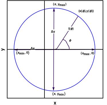
Deviation from circularity measures the amount of deviation from the circular shape of the shadow[93]. It is defined as follows:
| (55) | |||
| (56) | |||
| (57) |
In the above expression is the average radius of the shadow. is the length of the line joining the point on the shadow and the geometric centre (see 2). It must be noted that due to reflection symmetry of the Kerr-Sen metric, the shape of the shadow is symmetric about the -axis, hence the coordinate of the geometric center is 0. The coordinate of the geometric centre is calculated using the formula,
| (58) |
EHT observations of M87*:
The EHT collaboration measured the angular diameter , the axis ratio and the deviation from circularity for the image of M87*, the supermassive black hole candidate at the center of the galaxy M87 [7, 8, 9]. The values reported are given below:
- 1.
- 2.
- 3.
In order to determine the observationally favored Kerr-Sen parameter , we need to theoretically derive the above three observables as functions of the metric parameters and . As evident from 53 a theoretical computation of the angular diameter requires independent measurements of the black hole mass, distance and inclination (required to derive ). We use previously estimated masses and distance of this source to compute the theoretical angular diameter. The distance of M87* as reported from stellar population measurements turns out to be Mpc[107, 108, 109]. The angle of inclination which is the angle between the line of sight and the jet axis (the jet axis is believed to coincide with the spin axis of the black hole) is [110]. The mass of M87* has been measured using different methods. The mass measurement by modelling surface brightness and dispersion in stellar velocity was found to be [8, 111, 112]. Mass measurements from kinematic study of gas disk gives [8, 113]. Mass measured from the image of M87* by the EHT collaboration assuming general relativity turns out to be [7, 8, 9].
EHT observations of SgrA*:
In May 2022 the EHT collaboration released the image of the black hole SgrA* present at the galactic center of the Milky Way galaxy. The angular diameter of the image is found to be [13, 14, 15, 16, 17, 18]. The angular diameter of the shadow is [13, 14, 15, 16, 17, 18].
The mass and distance of SgrA* reported by the Keck collaboration keeping the redshift parameter free, are [114] and pc[114] respectively. Fixing the value of redshift parameter to unity the
mass and distance reported by the Keck team are and pc. The mass and distance of Sgr A* reported by the GRAVITY collaboration are and pc[115, 116] respectively. When systematics due to optical aberrations are taken into account the GRAVITY collaboration constrains the mass and distance of Sgr A* to and pc respectively. Apart from mass and distance we also need to provide independent measurements of the inclination angle to establish observational constrains on . From [117] we take (or equivalently ). When models based on extensive numerical simulations are compared with the the observed image of Sgr A*, one concludes that the inclination angle of the source is .
The estimates for axes ratio and the deviation from circularity for image of SgrA* by EHT collaboration are yet to be released, hence, for SgrA* the observable will only be used for estimating .
To constrain the Kerr-Sen/dilaton parameter using EHT observations, we proceed with the following approach:
- 1.
We derive the outline of the black hole shadow by calculating the impact parameters and for the Kerr-Sen black hole. We obtain the parametric equations of the black hole shadow outline.
- 2.
We fix the value of and vary the spin of black hole in suitable range such that event horizon radius is real and positive.
- 3.
For each combination of we calculate the values of angular diameter , axis ratio and the deviation from circularity . In these calculations we use values of mass , distance and inclination angle from previous measurements as discussed above.
- 4.
Then we repeat steps 2 and 3 for different values of upto . It must be noted that the dilaton parameter varies in the range since the horizon radius (in units of ) is given by which needs to be real and positive.
- 5.
After obtaining values for , and we plot contour plots for angular diameter , density plots for axes ratio and deviation from circularity as functions of and .
- 6.
The values of which are able to reproduce the observationally measured and give us the estimates of based on shadow related measurements.
Constrains on the dilaton parameter from EHT observations of M87* :
Here we discuss the observationally favored magnitude of the dilaton parameter derived from the shadow of M87* released by the Event Horizon Telescope collaboration in April 2019. In order to get an understanding of the observationally preferred value of we theoretically compute the observables, namely, (angular diameter), (axis ratio) and (deviation from circularity) related to the black hole shadow, which have been discussed towards the beginning of this section. It is important to recall that these observables depend on the metric parameters , and the inclination angle . In addition, the theoretically derived requires independent estimates of the mass and the distance of the black hole (see 53). The inclination angle is assumed to be and the distance is taken to be Mpc (obtained from stellar population measurements) throughout this discussion.
In 3a we plot the theoretical angular diameter of M87* as functions of and assuming mass (obtained from gas dynamics studies). We note from 3a that there is no suitable in the range 0 to 2 (obtained from the considerations of a real, positive event horizon) which can reproduce the observed angular diameter of M87* denoted by . Even when the maximum offset of 10% in the angular diameter is considered i.e is taken as the observed value, the mass falls short in addressing the observations. Since the theoretical angular diameter is directly proportional to the mass (53) therefore a larger mass of the source is required to reproduce the observations. Hence, it seems that the mass of M87* measured from gas dynamics studies needs to be revisited.


We next consider calculating the theoretical angular diameter of shadow of M87* keeping the distance fixed to Mpc but using the mass obtained from stellar dynamics measurements. With these values of mass and distance we evaluate the theoretical angular diameter for M87* which is plotted in 3b. From the figure it is evident that no value of can reproduce the observed image diameter . However, when maximum offset of 10% in the angular diameter is considered, is required to explain the observed angular diameter within 1- (, denoted by the red dashed line in 3b). Thus, when angular diameter is calculated with mass a non-zero can only explain the observations within 1- if maximum offset of 10% in the image diameter is allowed.
For completeness we also calculate the theoretical angular diameter with mass which is the mass derived by the EHT collaboration from the observed shadow of M87* assuming general relativity. Since this is the largest among all the three masses, it can explain the the observed image diameter of within 1- (39 denoted by the blue dashed line in 4). If the maximum offset of 10% is allowed then a non-zero dilaton charge can explain the observed shadow diameter (, denoted by the red solid line in 4). However, should not be used to infer the observationally favored magnitude of since this mass is obtained from shadow measurements assuming GR. Therefore, using this mass estimate we cannot constrain another alternative gravity theory.


We now discuss the constrains on from the other two observables and . The theoretical computation of these two observables does not require information about the mass and distance of the source. One however needs to provide the inclination angle of the source (which in the present case in ) to obtain and as functions of and . According to the EHT results, the deviation from circularity [7, 8, 9] or 0.1 for M87*. The density plot of for M87* is shown in 5a.
From the density plot we observe that for all values of spin and or 0.1 is realized. Thus, estimate for M87* does not give any additional bound on the Kerr-Sen parameter .
The EHT collaboration estimates an upper bound on the axis ratio for the image of M87*, i.e, [7, 8, 9]. The density plot for axes ratio in 5b indicate that for all values of and the axes ratio . Thus, EHT estimate of axes ratio for M87* does not provide any additional constrain on the dilaton parameter . It can be said that the axis ratio estimate allows non-zero values of Kerr-Sen parameter, although it does not constrain it.
Constrains on the dilaton parameter from EHT observations of Sgr A*:


The EHT collaboration measured the angular diameter for image of SgrA* to be while the shadow diameter is estimated to be [13, 14, 15, 16, 17, 18]. The theoretical angular diameter depends on the mass , the distance , the inclination angle and the metric parameters and (see 53). As before, we use previously determined masses and distances of the source to compute the theoretical angular diameter which is then compared with the observations to establish constrains on . The angle of inclination has an estimated upper bound obtained by comparing the image of Sgr A* with extensive numerical simulations [13]. Following [117] we fix the inclination angle to be for the present work.
In 6 the contours of theoretical angular diameter of the shadow of Sgr A* are plotted for different estimates of mass and distance. The mass and distance of the source have been well constrained by the Keck team and the GRAVITY collaboration. We first discuss the constrains on assuming distance and mass measurements by the Keck team [114]. Keeping the red-shift parameter free the mass and distance of Sgr A* turns out to be and pc, respectively. When the red-shift parameter is fixed to unity the distance and mass estimates by the Keck team yield pc and . In 6a and 6b we plot the contours of angular diameter of the shadow using the masses and distances estimated by the Keck team. From the figures it is evident that the observed shadow diameter of can be reproduced by (red solid line in 6a and 6b). When the lower 1- interval is considered, i.e., , then, can be as high as unity (red dashed line in 6a and 6b). Since the error bar associated with the shadow diameter is quite high () we do not assign much importance to this result but emphasize that a small but non-trivial value of is required to reproduce the central value of the observed shadow diameter. We further note that can explain the observed image diameter within 1-, (, blue dashed line in 6a and 6b).


We now discuss the constrains on the dilaton parameter from the distance and mass measurements by the GRAVITY collaboration [115, 116]. According to the results of the GRAVITY collaboration the mass and distance of Sgr A* turn out to be and pc[115, 116] respectively. However, when one takes into account the systematics due to optical aberrations, the GRAVITY collaboration constrains the mass and distance of Sgr A* to and pc respectively. In 6c and 6d we plot contours of theoretical angular diameter of shadow of Sgr A* assuming masses and distances reported by the GRAVITY collaboration. From the figures we note that once again a non-zero dilaton parameter is required to explain the central value of the observed shadow diameter of (red solid line in 6c and 6d). To reproduce the central value of the image diameter (blue solid line in 6c and 6d), a smaller but non-zero () is required. The upper 1- interval of the image diameter , (denoted by the blue dashed line in 6c and 6d) can be reproduced by . Therefore, for all mass and distance estimates of Sgr A*, a small positive dilaton charge is required to explain the observed shadow/image diameter. This implies that the observed shadow of Sgr A* can be better explained by the Kerr-Sen scenario.
For completeness we plot in 7 the dependence of the the deviation from circularity and the axis ratio on the metric parameters and . This is a theoretical plot which only requires independent estimate of the inclination of the source, which is taken to be as discussed earlier. EHT has not provided any data related to and for Sgr A*. These results therefore cannot impose additional constrains on the dilaton parameter at present. These plots can however be useful in future when EHT releases data pertaining to and for Sgr A*.
5 Concluding Remarks
In this work we investigate the signatures of Einstein-Maxwell dilaton-axion (EMDA) gravity in the shadows of Sgr A* and M87* observed by the Event Horizon Telescope collaboration. EMDA gravity arises in the low energy effective action of superstring theories and is associated with the dilaton and the axion fields coupled to the Maxwell field and the metric. Exploring the astrophysical implications of such a theory is important as it can potentially provide a possibility to test string inspired models. Moreover, the axion and dilaton fields are often invoked to address the inflationary paradigm or the present accelerated expansion of the universe [68, 69].
EMDA gravity is a scalar-vector-tensor theory of gravity that differs substantially from the standard general relativistic scenario. The stationary and axisymmetric black hole solution of EMDA gravity corresponds to the Kerr-Sen spacetime associated with the dilatonic charge and angular momentum acquired from the axionic field. The Maxwell field imparts electric charge to the Kerr-Sen black hole and in the absence of the Maxwell field the field strengths corresponding to dilaton and axion vanish. In that event the metric reduces to the Kerr background in general relativity. It is important to note that the charge of Kerr-Sen black hole originates from the axion-photon coupling and not from the charged particles falling onto the black hole.
In the present work we aim to constrain the charge of the Kerr-Sen black hole from observations related to black hole shadow. For this purpose we examine the motion of photons in the Kerr-Sen background and analyze the nature of the light rings and spherical photon orbits. These light rings when projected onto the observer’s sky give rise to the black hole shadow which depends sensitively on the background metric. The and coordinates of the shadow are dependent on the inclination angle and the two impact parameters and which denote the distances of the photon from the axis of rotation and the equatorial plane, respectively. These impact parameters in turn depend on the charge , the spin of the black hole and the radius of the spherical photon orbit . Thus, we have and as functions of , , and . The outline of the shadow is obtained by eliminating between and which is often achieved numerically. Since and also depend on , and , the shape and size of the shadow depend sensitively on these three parameters. For example, a rapidly rotating black hole viewed at a high inclination angle casts a non-circular shadow. In fact to observe a deviation from circularity in the shape of the shadow, one needs to have non-zero spin and inclination angle, both. The dilaton parameter on the other hand mainly has an impact on the shadow size. An increase in leads to a decrease in the shadow diameter.
Once the role of the metric on the shadow structure is derived we next compute the various observables associated with the black hole shadow. These include the angular diameter , the axis ratio and the deviation from circularity . Since the shadow is non-circular in general we can define a major axis and a minor axis associated with the shadow and a ratio of the two gives us the axis ratio . In order to theoretically compute these observables one need to provide estimates of the inclination angle of the source. Computation of further requires independent estimates of mass and distance of the compact object. For M87* and Sgr A* the mass, distance and inclination angle have been previously determined. We use these data to theoretically compute the observables pertaining to the shadow of M87* and Sgr A* which are eventually compared with observations to establish constrains on the dilaton parameter .
When the shadow of M87* is computed with predetermined mass , obtained from gas dynamics studies, the observed angular diameter cannot be reproduced for any value of , including which corresponds to the Kerr scenario. This mass measurement therefore possibly needs to be revisited. When mass determined from stellar dynamics measurements () is used, the observed shadow diameter can be reproduced by within 1- only when the maximum offset of 10% is considered. In both cases the distance is taken to be Mpc (obtained from stellar population measurements) to compute the theoretical shadow diameter. For completeness we also compute the shadow diameter with which is the mass reported by the EHT collaboration from the shadow measurements assuming GR. Since this mass is larger than the previous measurements, it can explain the observations better. However, theoretical shadow calculated using this mass should not be used to constrain as such a mass is derived from the observed shadow angular diameter assuming GR. With this mass therefore we cannot constrain another alternate gravity model. We note that with previously estimated masses the theoretical shadow is smaller than the observed one and since an increase in further shrinks the shadow, therefore the Kerr scenario can better explain the image of M87* compared to the Kerr-Sen scenario. It may be worthwhile to mention here that the Kerr solution is not unique to GR but arises even in several other alternative gravity scenarios. For example, the stationary, axisymmetric uncharged black hole solution in string theory resembles the Kerr solution in GR [74, 75]. We further mention that the Kerr scenario also fails to reproduce the observed shadow diameter of . Therefore, it seems that if in an alternate gravity model the shadow is larger than the GR scenario, it will better explain the observations, e.g. the braneworld scenario [96]. This may also be the reason why the mass of M87* obtained by the EHT collaboration is larger than the previous two measurements.
For Sgr A*, the mass and distance have been estimated independently by the Keck team and the GRAVITY collaboration. When the theoretical shadow is computed assuming mass and distance estimates by the Keck team, is required to explain the central value of the observed shadow diameter of . Further, is required to address the observed image diameter () within 1-. On considering mass and distance estimates by the GRAVITY collaboration, is required to reproduce the central value of the observed shadow diameter while is necessary to explain the central value of the observed image diameter. Thus, a small positive dilaton charge is required to address the observed shadow of Sgr A* for both the mass and distance estimates by the Keck team and the GRAVITY collaboration. The general relativistic scenario however can explain the observations when 1- interval is considered in the observed shadow diameter. Thus, the Kerr-Sen scenario better explains the observed shadow of Sgr A* compared to the Kerr scenario.
The charge of Kerr-Sen black hole has been constrained previously from different astrophysical observations, e.g. black hole continuum spectrum [118] and relativistic jets [119]. Comparison of the theoretical spectrum of eighty Palomar Green quasars with their optical observations reveal that best explains the observations. The general relativistic scenario with is however included when 1- interval is considered [118]. When the jet power associated with ballistic jets in microquasars is used to constrain the dilaton parameter, seem to be favored by observations [119]. Thus, we note that astrophysical observations, e.g, shadows, continuum spectra or jets either indicate a small dilatonic charge in black holes or exhibit a preference towards the Kerr scenario. All the observations rule out black holes with large dilaton charge. This is interesting as different astrophysical observations on completely different observational samples consistently indicate the same result. The scope to verify this finding will further increase as EHT releases more black hole images with greater resolution. The present astrophysical observations like quasi-periodic oscillations observed in the power spectrum of black holes or the Fe-line observed in the black hole spectrum can be further used to verify our result. This will be addressed in a future work.
Acknowledgements
Research of I.B. is funded by the Start-Up Research Grant from SERB, DST, Government of India (Reg. No. SRG/2021/000418).
References
- [1] S. Weinberg, Gravitation and Cosmology: Principles and Applications of the General Theory of Relativity. John Wiley and Sons, New York, 1972.
- [2] C. M. Will, “The Confrontation between General Relativity and Experiment,” Living Rev. Rel. 17 (2014) 4, arXiv:1403.7377 [gr-qc].
- [3] C. M. Will, Theory and experiment in gravitational physics. 1993.
- [4] LIGO Scientific, Virgo Collaboration, B. P. Abbott et al., “Observation of Gravitational Waves from a Binary Black Hole Merger,” Phys. Rev. Lett. 116 no. 6, (2016) 061102, arXiv:1602.03837 [gr-qc].
- [5] LIGO Scientific, Virgo Collaboration, B. P. Abbott et al., “GW170817: Observation of Gravitational Waves from a Binary Neutron Star Inspiral,” Phys. Rev. Lett. 119 no. 16, (2017) 161101, arXiv:1710.05832 [gr-qc].
- [6] LIGO Scientific, Virgo Collaboration, B. P. Abbott et al., “GWTC-1: A Gravitational-Wave Transient Catalog of Compact Binary Mergers Observed by LIGO and Virgo during the First and Second Observing Runs,” Phys. Rev. X 9 no. 3, (2019) 031040, arXiv:1811.12907 [astro-ph.HE].
- [7] Event Horizon Telescope Collaboration, K. Akiyama et al., “First M87 Event Horizon Telescope Results. I. The Shadow of the Supermassive Black Hole,” Astrophys. J. Lett. 875 (2019) L1, arXiv:1906.11238 [astro-ph.GA].
- [8] Event Horizon Telescope Collaboration, K. Akiyama et al., “First M87 Event Horizon Telescope Results. VI. The Shadow and Mass of the Central Black Hole,” Astrophys. J. Lett. 875 no. 1, (2019) L6, arXiv:1906.11243 [astro-ph.GA].
- [9] Event Horizon Telescope Collaboration, K. Akiyama et al., “First M87 Event Horizon Telescope Results. V. Physical Origin of the Asymmetric Ring,” Astrophys. J. Lett. 875 no. 1, (2019) L5, arXiv:1906.11242 [astro-ph.GA].
- [10] Event Horizon Telescope Collaboration, K. Akiyama et al., “First M87 Event Horizon Telescope Results. II. Array and Instrumentation,” Astrophys. J. Lett. 875 no. 1, (2019) L2, arXiv:1906.11239 [astro-ph.IM].
- [11] Event Horizon Telescope Collaboration, K. Akiyama et al., “First M87 Event Horizon Telescope Results. III. Data Processing and Calibration,” Astrophys. J. Lett. 875 no. 1, (2019) L3, arXiv:1906.11240 [astro-ph.GA].
- [12] Event Horizon Telescope Collaboration, K. Akiyama et al., “First M87 Event Horizon Telescope Results. IV. Imaging the Central Supermassive Black Hole,” Astrophys. J. Lett. 875 no. 1, (2019) L4, arXiv:1906.11241 [astro-ph.GA].
- [13] Event Horizon Telescope Collaboration, K. Akiyama et al., “First Sagittarius A* Event Horizon Telescope Results. I. The Shadow of the Supermassive Black Hole in the Center of the Milky Way,” Astrophys. J. Lett. 930 no. 2, (2022) L12.
- [14] Event Horizon Telescope Collaboration, K. Akiyama et al., “First Sagittarius A* Event Horizon Telescope Results. II. EHT and Multiwavelength Observations, Data Processing, and Calibration,” Astrophys. J. Lett. 930 no. 2, (2022) L13.
- [15] Event Horizon Telescope Collaboration, K. Akiyama et al., “First Sagittarius A* Event Horizon Telescope Results. III. Imaging of the Galactic Center Supermassive Black Hole,” Astrophys. J. Lett. 930 no. 2, (2022) L14.
- [16] Event Horizon Telescope Collaboration, K. Akiyama et al., “First Sagittarius A* Event Horizon Telescope Results. IV. Variability, Morphology, and Black Hole Mass,” Astrophys. J. Lett. 930 no. 2, (2022) L15.
- [17] Event Horizon Telescope Collaboration, K. Akiyama et al., “First Sagittarius A* Event Horizon Telescope Results. V. Testing Astrophysical Models of the Galactic Center Black Hole,” Astrophys. J. Lett. 930 no. 2, (2022) L16.
- [18] Event Horizon Telescope Collaboration, K. Akiyama et al., “First Sagittarius A* Event Horizon Telescope Results. VI. Testing the Black Hole Metric,” Astrophys. J. Lett. 930 no. 2, (2022) L17.
- [19] R. Penrose, “Gravitational collapse and space-time singularities,” Phys. Rev. Lett. 14 (1965) 57–59.
- [20] S. W. Hawking, “Breakdown of Predictability in Gravitational Collapse,” Phys. Rev. D14 (1976) 2460–2473.
- [21] S. W. Hawking and G. F. R. Ellis, The Large Scale Structure of Space-Time. Cambridge Monographs on Mathematical Physics. Cambridge University Press, 2, 2011.
- [22] R. M. Wald, General Relativity. Chicago Univ. Pr., Chicago, USA, 1984.
- [23] D. Christodoulou, “The formation of black holes and singularities in spherically symmetric gravitational collapse,” Commun. Pure Appl. Math. 44 no. 3, (1991) 339–373.
- [24] C. Rovelli, “Black hole entropy from loop quantum gravity,” Phys. Rev. Lett. 77 (1996) 3288–3291, arXiv:gr-qc/9603063 [gr-qc].
- [25] F. Dowker, “Causal sets and the deep structure of spacetime,” in 100 Years Of Relativity: space-time structure: Einstein and beyond, A. Ashtekar, ed., pp. 445–464. 2005. arXiv:gr-qc/0508109 [gr-qc].
- [26] A. Ashtekar, T. Pawlowski, and P. Singh, “Quantum nature of the big bang,” Phys. Rev. Lett. 96 (2006) 141301, arXiv:gr-qc/0602086 [gr-qc].
- [27] D. Kothawala, “Minimal Length and Small Scale Structure of Spacetime,” Phys. Rev. D88 no. 10, (2013) 104029, arXiv:1307.5618 [gr-qc].
- [28] E. P. Wigner, The Basic Conflict Between the Concepts of General Relativity and of Quantum Mechanics, pp. 350–350. Springer Berlin Heidelberg, Berlin, Heidelberg, 1997. https://doi.org/10.1007/978-3-662-09203-3_33.
- [29] M. Milgrom, “A Modification of the Newtonian dynamics: Implications for galaxies,” Astrophys. J. 270 (1983) 371–383.
- [30] J. Bekenstein and M. Milgrom, “Does the missing mass problem signal the breakdown of Newtonian gravity?,” Astrophys. J. 286 (1984) 7–14.
- [31] M. Milgrom and R. H. Sanders, “MOND and the Dearth of dark matter in ordinary elliptical galaxies’,” Astrophys. J. 599 (2003) L25–L28, arXiv:astro-ph/0309617 [astro-ph].
- [32] T. Clifton, P. G. Ferreira, A. Padilla, and C. Skordis, “Modified Gravity and Cosmology,” Phys. Rept. 513 (2012) 1–189, arXiv:1106.2476 [astro-ph.CO].
- [33] Supernova Cosmology Project Collaboration, S. Perlmutter et al., “Measurements of and from 42 high redshift supernovae,” Astrophys. J. 517 (1999) 565–586, arXiv:astro-ph/9812133.
- [34] Supernova Search Team Collaboration, A. G. Riess et al., “Observational evidence from supernovae for an accelerating universe and a cosmological constant,” Astron. J. 116 (1998) 1009–1038, arXiv:astro-ph/9805201.
- [35] T. P. Sotiriou and V. Faraoni, “f(R) Theories Of Gravity,” Rev. Mod. Phys. 82 (2010) 451–497, arXiv:0805.1726 [gr-qc].
- [36] A. De Felice and S. Tsujikawa, “f(R) theories,” Living Rev. Rel. 13 (2010) 3, arXiv:1002.4928 [gr-qc].
- [37] S. Capozziello and M. De Laurentis, “Extended Theories of Gravity,” Phys. Rept. 509 (2011) 167–321, arXiv:1108.6266 [gr-qc].
- [38] R. Maartens, “Brane world gravity,” Living Rev. Rel. 7 (2004) 7, arXiv:gr-qc/0312059 [gr-qc].
- [39] J. M. Overduin and P. S. Wesson, “Kaluza-Klein gravity,” Phys. Rept. 283 (1997) 303–380, arXiv:gr-qc/9805018.
- [40] T. Kobayashi, “Horndeski theory and beyond: a review,” Rept. Prog. Phys. 82 no. 8, (2019) 086901, arXiv:1901.07183 [gr-qc].
- [41] R. T. Hammond, “Torsion gravity,” Rept. Prog. Phys. 65 (2002) 599–649.
- [42] E. Berti et al., “Testing General Relativity with Present and Future Astrophysical Observations,” Class. Quant. Grav. 32 (2015) 243001, arXiv:1501.07274 [gr-qc].
- [43] D. Psaltis, “Probes and Tests of Strong-Field Gravity with Observations in the Electromagnetic Spectrum,” Living Rev. Rel. 11 (2008) 9, arXiv:0806.1531 [astro-ph].
- [44] S. Nojiri and S. D. Odintsov, “Modified gravity with negative and positive powers of the curvature: Unification of the inflation and of the cosmic acceleration,” Phys.Rev. D68 (2003) 123512, arXiv:hep-th/0307288 [hep-th].
- [45] S. Nojiri and S. D. Odintsov, “Modified f(R) gravity consistent with realistic cosmology: From matter dominated epoch to dark energy universe,” Phys. Rev. D74 (2006) 086005, arXiv:hep-th/0608008 [hep-th].
- [46] S. Capozziello, S. Nojiri, S. D. Odintsov, and A. Troisi, “Cosmological viability of f(R)-gravity as an ideal fluid and its compatibility with a matter dominated phase,” Phys. Lett. B639 (2006) 135–143, arXiv:astro-ph/0604431 [astro-ph].
- [47] C. Lanczos, “Electricity as a natural property of Riemannian geometry,” Rev. Mod. Phys. 39 (1932) 716–736.
- [48] C. Lanczos, “A Remarkable property of the Riemann-Christoffel tensor in four dimensions,” Annals Math. 39 (1938) 842–850.
- [49] D. Lovelock, “The einstein tensor and its generalizations,” Journal of Mathematical Physics 12 no. 3, (1971) 498–501.
- [50] T. Padmanabhan and D. Kothawala, “Lanczos-Lovelock models of gravity,” Phys. Rept. 531 (2013) 115–171, arXiv:1302.2151 [gr-qc].
- [51] T. Shiromizu, K.-i. Maeda, and M. Sasaki, “The Einstein equation on the 3-brane world,” Phys. Rev. D62 (2000) 024012, arXiv:gr-qc/9910076 [gr-qc].
- [52] N. Dadhich, R. Maartens, P. Papadopoulos, and V. Rezania, “Black holes on the brane,” Phys. Lett. B487 (2000) 1–6, arXiv:hep-th/0003061 [hep-th].
- [53] T. Harko and M. K. Mak, “Vacuum solutions of the gravitational field equations in the brane world model,” Phys. Rev. D69 (2004) 064020, arXiv:gr-qc/0401049 [gr-qc].
- [54] T. R. P. Carames, M. E. X. Guimaraes, and J. M. Hoff da Silva, “Effective gravitational equations for braneworld models,” Phys. Rev. D87 no. 10, (2013) 106011, arXiv:1205.4980 [gr-qc].
- [55] T. Kobayashi, T. Shiromizu, and N. Deruelle, “Low energy effective gravitational equations on a Gauss-Bonnet brane,” Phys. Rev. D74 (2006) 104031, arXiv:hep-th/0608166 [hep-th].
- [56] S. Chakraborty and S. SenGupta, “Spherically symmetric brane spacetime with bulk gravity,” Eur. Phys. J. C75 no. 1, (2015) 11, arXiv:1409.4115 [gr-qc].
- [57] S. Chakraborty and S. SenGupta, “Effective gravitational field equations on -brane embedded in n-dimensional bulk of Einstein and gravity,” Eur. Phys. J. C75 no. 11, (2015) 538, arXiv:1504.07519 [gr-qc].
- [58] G. W. Horndeski, “Second-order scalar-tensor field equations in a four-dimensional space,” Int. J. Theor. Phys. 10 (1974) 363–384.
- [59] T. P. Sotiriou and S.-Y. Zhou, “Black hole hair in generalized scalar-tensor gravity,” Phys. Rev. Lett. 112 (2014) 251102, arXiv:1312.3622 [gr-qc].
- [60] E. Babichev, C. Charmousis, and A. Lehébel, “Black holes and stars in Horndeski theory,” Class. Quant. Grav. 33 no. 15, (2016) 154002, arXiv:1604.06402 [gr-qc].
- [61] C. Charmousis and M. Tsoukalas, “Lovelock Galileons and black holes,” Phys. Rev. D92 no. 10, (2015) 104050, arXiv:1506.05014 [gr-qc].
- [62] S. Bhattacharya and S. Chakraborty, “Constraining some Horndeski gravity theories,” Phys. Rev. D95 no. 4, (2017) 044037, arXiv:1607.03693 [gr-qc].
- [63] P. Horava and E. Witten, “Heterotic and type I string dynamics from eleven-dimensions,” Nucl. Phys. B460 (1996) 506–524, arXiv:hep-th/9510209 [hep-th]. [,397(1995)].
- [64] P. Horava and E. Witten, “Eleven-dimensional supergravity on a manifold with boundary,” Nucl. Phys. B475 (1996) 94–114, arXiv:hep-th/9603142 [hep-th].
- [65] J. Polchinski, String theory. Vol. 1: An introduction to the bosonic string. Cambridge Monographs on Mathematical Physics. Cambridge University Press, 2007.
- [66] J. Polchinski, String theory. Vol. 2: Superstring theory and beyond. Cambridge Monographs on Mathematical Physics. Cambridge University Press, 2007.
- [67] A. Sen, “Rotating charged black hole solution in heterotic string theory,” Phys. Rev. Lett. 69 (1992) 1006–1009, arXiv:hep-th/9204046.
- [68] J. Sonner and P. K. Townsend, “Recurrent acceleration in dilaton-axion cosmology,” Phys. Rev. D 74 (2006) 103508, arXiv:hep-th/0608068.
- [69] R. Catena and J. Moller, “Axion-dilaton cosmology and dark energy,” JCAP 03 (2008) 012, arXiv:0709.1931 [hep-ph].
- [70] G. Gibbons and K.-i. Maeda, “Black Holes and Membranes in Higher Dimensional Theories with Dilaton Fields,” Nucl. Phys. B 298 (1988) 741–775.
- [71] D. Garfinkle, G. T. Horowitz, and A. Strominger, “Charged black holes in string theory,” Phys. Rev. D 43 (1991) 3140. [Erratum: Phys.Rev.D 45, 3888 (1992)].
- [72] G. T. Horowitz and A. Strominger, “Black strings and P-branes,” Nucl. Phys. B 360 (1991) 197–209.
- [73] R. Kallosh and T. Ortin, “Charge quantization of axion - dilaton black holes,” Phys. Rev. D 48 (1993) 742–747, arXiv:hep-th/9302109.
- [74] K. S. Thorne, R. Price, and D. Macdonald, eds., BLACK HOLES: THE MEMBRANE PARADIGM. 1986.
- [75] D. Psaltis, D. Perrodin, K. R. Dienes, and I. Mocioiu, “Kerr Black Holes are Not Unique to General Relativity,” Phys. Rev. Lett. 100 (2008) 091101, arXiv:0710.4564 [astro-ph].
- [76] K. Hioki and U. Miyamoto, “Hidden symmetries, null geodesics, and photon capture in the Sen black hole,” Phys. Rev. D 78 (2008) 044007, arXiv:0805.3146 [gr-qc].
- [77] P. Pradhan, “Thermodynamic Products for Sen Black Hole,” Eur. Phys. J. C 76 no. 3, (2016) 131, arXiv:1503.04514 [gr-qc].
- [78] M. Guo, S. Song, and H. Yan, “Observational signature of a near-extremal Kerr-Sen black hole in the heterotic string theory,” Phys. Rev. D 101 no. 2, (2020) 024055, arXiv:1911.04796 [gr-qc].
- [79] R. Uniyal, H. Nandan, and K. D. Purohit, “Null geodesics and observables around the Kerr–Sen black hole,” Class. Quant. Grav. 35 no. 2, (2018) 025003, arXiv:1703.07510 [gr-qc].
- [80] G. N. Gyulchev and S. S. Yazadjiev, “Kerr-Sen dilaton-axion black hole lensing in the strong deflection limit,” Phys. Rev. D 75 (2007) 023006, arXiv:gr-qc/0611110.
- [81] J. An, J. Peng, Y. Liu, and X.-H. Feng, “Kerr-Sen Black Hole as Accelerator for Spinning Particles,” Phys. Rev. D 97 no. 2, (2018) 024003, arXiv:1710.08630 [gr-qc].
- [82] Z. Younsi, A. Zhidenko, L. Rezzolla, R. Konoplya, and Y. Mizuno, “New method for shadow calculations: Application to parametrized axisymmetric black holes,” Phys. Rev. D 94 no. 8, (2016) 084025, arXiv:1607.05767 [gr-qc].
- [83] Y. Mizuno, Z. Younsi, C. M. Fromm, O. Porth, M. De Laurentis, H. Olivares, H. Falcke, M. Kramer, and L. Rezzolla, “The Current Ability to Test Theories of Gravity with Black Hole Shadows,” Nat. Astron. 2 no. 7, (2018) 585–590, arXiv:1804.05812 [astro-ph.GA].
- [84] S. V. M. C. B. Xavier, P. V. P. Cunha, L. C. B. Crispino, and C. A. R. Herdeiro, “Shadows of charged rotating black holes: Kerr–Newman versus Kerr–Sen,” Int. J. Mod. Phys. D 29 no. 11, (2020) 2041005, arXiv:2003.14349 [gr-qc].
- [85] S. Jana and S. Kar, “Shadows in dyonic Kerr-Sen black holes,” arXiv:2303.14513 [gr-qc].
- [86] M. Rogatko, “Positivity of energy in Einstein-Maxwell axion dilaton gravity,” Class. Quant. Grav. 19 (2002) 5063–5072, arXiv:hep-th/0209126.
- [87] C. Ganguly and S. SenGupta, “Penrose process in a charged axion–dilaton coupled black hole,” Eur. Phys. J. C 76 no. 4, (2016) 213, arXiv:1401.6826 [hep-th].
- [88] A. Garcia, D. Galtsov, and O. Kechkin, “Class of stationary axisymmetric solutions of the Einstein-Maxwell dilaton - axion field equations,” Phys. Rev. Lett. 74 (1995) 1276–1279.
- [89] A. Ghezelbash and H. Siahaan, “Hidden and Generalized Conformal Symmetry of Kerr-Sen Spacetimes,” Class. Quant. Grav. 30 (2013) 135005, arXiv:1206.0714 [hep-th].
- [90] C. Bernard, “Stationary charged scalar clouds around black holes in string theory,” Phys. Rev. D 94 no. 8, (2016) 085007, arXiv:1608.05974 [gr-qc].
- [91] S. Yazadjiev, “Exact static solutions in four-dimensional Einstein-Maxwell dilaton gravity,” Int. J. Mod. Phys. D 8 (1999) 635–643, arXiv:gr-qc/9906048.
- [92] S. E. Gralla, D. E. Holz, and R. M. Wald, “Black Hole Shadows, Photon Rings, and Lensing Rings,” Phys. Rev. D100 no. 2, (2019) 024018, arXiv:1906.00873 [astro-ph.HE].
- [93] C. Bambi, K. Freese, S. Vagnozzi, and L. Visinelli, “Testing the rotational nature of the supermassive object M87* from the circularity and size of its first image,” Phys. Rev. D100 no. 4, (2019) 044057, arXiv:1904.12983 [gr-qc].
- [94] K. Hioki and K.-i. Maeda, “Measurement of the Kerr Spin Parameter by Observation of a Compact Object’s Shadow,” Phys. Rev. D80 (2009) 024042, arXiv:0904.3575 [astro-ph.HE].
- [95] S. Vagnozzi and L. Visinelli, “Hunting for extra dimensions in the shadow of M87*,” Phys. Rev. D100 no. 2, (2019) 024020, arXiv:1905.12421 [gr-qc].
- [96] I. Banerjee, S. Chakraborty, and S. SenGupta, “Silhouette of M87*: A New Window to Peek into the World of Hidden Dimensions,” Phys. Rev. D 101 no. 4, (2020) 041301, arXiv:1909.09385 [gr-qc].
- [97] P. V. P. Cunha and C. A. R. Herdeiro, “Shadows and strong gravitational lensing: a brief review,” Gen. Rel. Grav. 50 no. 4, (2018) 42, arXiv:1801.00860 [gr-qc].
- [98] A. de Vries, “The apparent shape of a rotating charged black hole, closed photon orbits and the bifurcation setA4,” Classical and Quantum Gravity 17 no. 1, (Dec, 1999) 123–144. https://doi.org/10.1088%2F0264-9381%2F17%2F1%2F309.
- [99] P. V. P. Cunha, C. A. R. Herdeiro, and M. J. Rodriguez, “Does the black hole shadow probe the event horizon geometry?,” Phys. Rev. D97 no. 8, (2018) 084020, arXiv:1802.02675 [gr-qc].
- [100] R. Roy and U. A. Yajnik, “Evolution of black hole shadow in the presence of ultralight bosons,” arXiv:1906.03190 [gr-qc].
- [101] J. M. Bardeen, “Timelike and null geodesics in the Kerr metric,” in Proceedings, Ecole d’Eté de Physique Théorique: Les Astres Occlus: Les Houches, France, August, 1972, pp. 215–240. 1973.
- [102] B. Carter, “Global structure of the Kerr family of gravitational fields,” Phys. Rev. 174 (1968) 1559–1571.
- [103] N. Tsukamoto, Z. Li, and C. Bambi, “Constraining the spin and the deformation parameters from the black hole shadow,” JCAP 06 (2014) 043, arXiv:1403.0371 [gr-qc].
- [104] L. Balart and E. C. Vagenas, “Regular black holes with a nonlinear electrodynamics source,” Phys. Rev. D 90 no. 12, (2014) 124045, arXiv:1408.0306 [gr-qc].
- [105] M. Amir and S. G. Ghosh, “Shapes of rotating nonsingular black hole shadows,” Phys. Rev. D 94 no. 2, (2016) 024054, arXiv:1603.06382 [gr-qc].
- [106] N. Tsukamoto, “Black hole shadow in an asymptotically-flat, stationary, and axisymmetric spacetime: The Kerr-Newman and rotating regular black holes,” Phys. Rev. D 97 no. 6, (2018) 064021, arXiv:1708.07427 [gr-qc].
- [107] S. Bird, W. E. Harris, J. P. Blakeslee, and C. Flynn, “The Inner Halo of M87: A First Direct View of the Red-Giant Population,” Astron. Astrophys. 524 (2010) A71, arXiv:1009.3202 [astro-ph.GA].
- [108] J. P. Blakeslee, A. Jordan, S. Mei, P. Cote, L. Ferrarese, L. Infante, E. W. Peng, J. L. Tonry, and M. J. West, “The ACS Fornax Cluster Survey. V. Measurement and Recalibration of Surface Brightness Fluctuations and a Precise Value of the Fornax–Virgo Relative Distance,” Astrophys. J. 694 (2009) 556–572, arXiv:0901.1138 [astro-ph.CO].
- [109] M. Cantiello et al., “A Precise Distance to the Host Galaxy of the Binary Neutron Star Merger GW170817 Using Surface Brightness Fluctuations,” Astrophys. J. 854 no. 2, (2018) L31, arXiv:1801.06080 [astro-ph.GA].
- [110] R. Craig Walker, P. E. Hardee, F. B. Davies, C. Ly, and W. Junor, “The Structure and Dynamics of the Subparsec Jet in M87 Based on 50 VLBA Observations over 17 Years at 43 GHz,” Astrophys. J. 855 no. 2, (2018) 128, arXiv:1802.06166 [astro-ph.HE].
- [111] K. Gebhardt and J. Thomas, “The Black Hole Mass, Stellar M/L, and Dark Halo in M87,” Astrophys. J. 700 (2009) 1690–1701, arXiv:0906.1492 [astro-ph.CO].
- [112] K. Gebhardt et al., “A Relationship between nuclear black hole mass and galaxy velocity dispersion,” Astrophys. J. 539 (2000) L13, arXiv:astro-ph/0006289 [astro-ph].
- [113] J. L. Walsh, A. J. Barth, L. C. Ho, and M. Sarzi, “The M87 Black Hole Mass from Gas-dynamical Models of Space Telescope Imaging Spectrograph Observations,” Astrophys. J. 770 (2013) 86, arXiv:1304.7273 [astro-ph.CO].
- [114] T. Do et al., “Relativistic redshift of the star S0-2 orbiting the Galactic center supermassive black hole,” Science 365 no. 6454, (2019) 664–668, arXiv:1907.10731 [astro-ph.GA].
- [115] GRAVITY Collaboration, R. Abuter et al., “Mass distribution in the Galactic Center based on interferometric astrometry of multiple stellar orbits,” Astron. Astrophys. 657 (2022) L12, arXiv:2112.07478 [astro-ph.GA].
- [116] GRAVITY Collaboration, R. Abuter et al., “Detection of the Schwarzschild precession in the orbit of the star S2 near the Galactic centre massive black hole,” Astron. Astrophys. 636 (2020) L5, arXiv:2004.07187 [astro-ph.GA].
- [117] Török, G., Abramowicz, M. A., Klu´zniak, W., and Stuchlík, Z., “The orbital resonance model for twin peak khz quasi periodic oscillations in microquasars,” A&A 436 no. 1, (2005) 1–8. https://doi.org/10.1051/0004-6361:20047115.
- [118] I. Banerjee, B. Mandal, and S. SenGupta, “Implications of Einstein–Maxwell dilaton–axion gravity from the black hole continuum spectrum,” Mon. Not. Roy. Astron. Soc. 500 no. 1, (2020) 481–492, arXiv:2007.13980 [gr-qc].
- [119] I. Banerjee, B. Mandal, and S. SenGupta, “Signatures of Einstein-Maxwell dilaton-axion gravity from the observed jet power and the radiative efficiency,” Phys. Rev. D 103 no. 4, (2021) 044046, arXiv:2007.03947 [gr-qc].