Formation of the warped debris disc around Pictoris2023Formation of the warped debris disc around Pictoris–B
Abstract
In light of the recent confirmation of an eccentric orbit giant planet, Pic c, I revisit the formation and evolution of the warped debris disc in the system. Pic c is interior to Pic b, and the debris disc is exterior to both planets. Previous -body simulations have shown that Pic b is responsible for exciting the inclination of the debris disc. With hydrodynamical simulations, I model a protoplanetary gas disc misaligned with the planets. I find that the gas disc does not exhibit significant long lasting inclination excitation from the planets even for the observed disc size. The warp that is excited by the planets propagates through the entire disc with a timescale much less than the gas disc lifetime. Therefore, the observed warp in the debris disc must be produced after the gas disc has dispersed. With analytical secular theory calculations, I show that two secular resonances are exterior to Pic b, located at and . This agrees with my -body simulations that show that these secular resonances shape the inner edge of the Pic debris disc at a radius that agrees with observations.
Keywords:
stars: Pictoris – planet-disc interactions – protoplanetary discs1 Introduction
Planetary systems that house debris discs are exceptional laboratories for studying the effects of planetary dynamics. Studying the composition and structure of debris discs can lead to information on exoplanets, such as the compositions, masses, and orbits (Hughes et al. 2018). The occurrence rate of debris discs around A and F stars is estimated at per cent, while the rate is per cent around G and K type stars (Su et al. 2006; Hillenbrand et al. 2008; Trilling et al. 2008; Sibthorpe et al. 2018). Studying debris disc evolution and structure will shed light on the origin of planetary systems.
One such planetary system that has been widely studied is the Pictoris (Pic) system. Pic is a young A6V-type star with an age of (Shkolnik et al. 2012; Binks & Jeffries 2014; Bell et al. 2015; Miret-Roig et al. 2020) at a distance of 19.45 ± 0.05 pc (van Leeuwen 2007). The mass of Pic is estimated to be (Wang et al. 2016), with a stellar diameter of (Defrère et al. 2012) and a projected rotation velocity of (Royer et al. 2007).
Pic b was one of the first exoplanets to be discovered using direct imaging (Lagrange et al. 2009; Lagrange et al. 2010, e.g.,). Further observations of this planet include photometry spanning the near-infrared (Quanz et al. 2010; Bonnefoy et al. 2011; Currie et al. 2011; Bonfils et al. 2013; Males et al. 2014; Morzinski et al. 2015), low-resolution spectroscopy (Chilcote et al. 2015; Chilcote et al. 2017), and medium-resolution spectroscopy (Snellen et al. 2014; Gravity Collaboration et al. 2020). The dynamical mass measurements of Pic b were derived from the observations from Hipparcos (van Leeuwen 2007) and Gaia (Gaia Collaboration et al. 2016; Lindegren et al. 2018). Lagrange et al. 2020 refined the mass measurements using SPHERE, GRAVITY, and RV data. Recently, the works of Nowak et al. 2020 and Brandt et al. 2021 estimate a planet mass of with a semi-major axis of . The recent confirmation of a second planet in the Pic system, Pic c (Lagrange et al. 2019; Nowak et al. 2020), has now fueled further investigation of the planetary dynamics occurring in this system. Pic c has a dynamical mass of with a semi-major axis of (Nowak et al. 2020; Brandt et al. 2021). Table 1 shows the orbital elements for Pic b and Pic c from the work of Brandt et al. 2021. Both planets are on eccentric orbits with eccentricities of and for Pic b and Pic c, respectively. Moreover, the planets are coplanar to one another and viewed nearly in an edge-on geometry.
| Planet Parameters | Symbol | Pictoris b | Pictoris c | Unit |
|---|---|---|---|---|
| Semi-major axis | ||||
| Eccentricity axis | – | |||
| Inclination | ||||
| PA of ascending node | ||||
| Argument of periastron | ||||
| Planet mass | ||||
| Period |
A bright edge-on circumstellar debris disc around Pic was first imaged in the mid-1980’s (Smith & Terrile 1984). On top of this, spectroscopic observations reveal a high rate of transits of small evaporating exocomets (Kiefer et al. 2014). The presence of Pic b is thought to explain the infalling exocomets, given that the planet has a nonzero eccentricity (Beust & Morbidelli 1996; Beust & Morbidelli 2000, e.g.,). Adaptive optics coronographic images of the Pic disc detected the disc in the near-infrared (NIR) through scattered light down to from the star (Mouillet et al. 1997b). The Hubble Space Telescope (HST) also resolved the disc down to (Burrows et al. 1995; Lecavelier Des Etangs et al. 1997). The observed outer radius of the debris disc may extend out to of au (Janson et al. 2021). The most intriguing structural anomaly of the debris disc is a major asymmetric feature found at around . The disc displays a warp at this location where there is a offset between the warped inner disc and the outer main disc (Kalas & Jewitt 1995; Wahhaj et al. 2003; Weinberger et al. 2003; Golimowski et al. 2006; Nielsen et al. 2014). Kraus et al. 2020 investigated the spin-orbit alignment of the planetary orbit of Pic b. To accomplish this, they measured the mutual inclination angle between the angular momentum vectors of the stellar photosphere and the planetary orbit. They found that the planetary orbit for Pic b is inclined by . Moreover, recent observations estimated that the orbit of Pic c is nearly coplanar to Pic b (Nowak et al. 2020; Brandt et al. 2021). Misalignment of a planet to the spin-axis of the central star can arise from dynamical mechanisms, including planet-planet scattering (Chatterjee et al. 2008). Alternatively, the protoplanetary disc around a single star may be misaligned during the planet formation stage (Bate et al. 2010; Lai et al. 2011; Rogers & Lin 2013; Fielding et al. 2015, e.g.,).
An inclined planet was proposed to trigger the warp structure in the debris disc (Mouillet et al. 1997a). Dawson et al. 2011 investigated the warp in the Pic debris disc utilizing –body simulations and secular theory. At this time, only Pic b was known. They found that the low-inclination planet, Pic b, causes a forced inclination excitation within the debris disc at around . They concluded that the inclination of the observed inner disc is solely due to Pic b because if Pic b were aligned with the flat outer disc (which observations suggested), it would prevent another planet from creating a warp. More recently, Dong et al. 2020 ran numerical simulations comparing the pic debris disc structure under the influence of one and two planets. They found that the inclusion of Pic C does not significantly affect the warped debris disc structure.
In this work, I further investigate how the dynamics of the newly confirmed inner planet and the outer planet in the Pic system affect the debris disc. I consider the dynamics of the protoplanetary gas disc that the planets and the debris disc would have originally formed in and the dynamics of the observed debris disc. The main point I want to address is whether the warp in the debris disc could have formed during the protoplanetary disc phase. In Section 2, I discuss the setup for my hydrodynamical and –body simulations. In Section 3, I show the results of my hydrodynamical simulations. In Section 4, I apply a secular resonance model to estimate the location of secular resonances, and compare that to the –body simulations. Finally, I draw my conclusions in Section 5.
2 Numerical Methods
To simulate the Pic system, I use both hydrodynamical and –body simulations. The former is used to model the gas disc phase, and the latter is used to model the debris disc phase.
2.1 Hydrodynamical setup
I use the 3-dimensional smoothed particle hydrodynamics (SPH) code phantom (Price et al. 2018) to model a gas-only protoplanetary disc around Pic. I consider a gas disc in the bending-wave regime, where the disc aspect ratio is larger than the viscosity coefficient. The gas disc initially consists of equal-mass Lagrangian particles that are distributed between the inner disc radius, and the outer disc radius, . The inner disc radius is selected based on the observed data, in that there is little material detected at (Burrows et al. 1995; Lecavelier Des Etangs et al. 1997). In the simulation, material is able to flow inwards. In order to save computational time and increase resolution, I initially truncate the outer edge of the gas disc. I note that the truncated outer radius maintains the angular momentum equilibrium, meaning that the outer disc still bears most of the angular momentum. I also simulate two larger radial discs, and . To ensure that these extended disc sizes have the same resolution as the narrow disc, I increase the number of particles to for and for . Note that the observed disc size around Pic may be on the order of (Janson et al. 2021).
The gas surface density profile is initially set as a power law distribution given by
| (1) |
where is the density normalization and is the power law index. Note that the density normalization is set from the total disc mass, . I select a value of . The disc mass is set at . Observational study of the CO gas in the primordial debris disc derives an upper mass of (Hales et al. 2019), however, I expect the mass of the primordially gaseous circumstellar disc to be higher. The equation of state is locally isothermal and scaled to the thickness of the disc with sound speed given by
| (2) |
where and is the sound speed. I take and the disc aspect ratio is set to at . The physical disc viscosity is modelled using the artificial viscosity , implemented in phantom (Lodato & Price 2010), given by
| (3) |
where is the mean smoothing length on particles in a cylindrical ring at a given radius (Artymowicz & Lubow 1994; Murray 1996; Lodato & Pringle 2007). I assume a value of disc viscosity , which gives . With this value of , the disc is resolved with a shell-averaged smoothing length per scale height of . Using the above values for and ensures that the disc is uniformly resolved, meaning that and consequently are constant over the radial extent of the disc (Lodato & Pringle 2007, e.g.,).
The central star is modelled as a sink particle with an accretion radius of . This accretion radius is considered a hard boundary, where particles that penetrate this radius are per cent accreted, and the mass and angular momentum of the particles are added to the star. Furthermore, I include the two eccentric Pic planets, Pic b and Pic c. The planets have an initial semi-major axis, eccentricity, and mass given in Table 1 using the observations of Brandt et al. 2021. The planets both begin at apastron. The semi-major axes of the planets are interior to inner disc edge, and thus are not embedded within the disc. However, the inner edge of the disc will subsequently viciously extend inward during the simulation and will begin interacting will the planets (see Appendix A for more details). Observational estimates of the present-day tilts of the planets are (Kraus et al. 2020, e.g.,). Planets on inclined orbits will damp back to coplanar due to viscous interactions with the disc (Tanaka et al. 2002, e.g.,). I simulate two scenarios where the initial mutual inclination between the planets’ and disc’s angular momentum vectors are and , which are larger than the present-day misalignment. The planetary accretion radius is equal to the central star to speed up computational time. When , the simulation in considered unresolved. Therefore, I stop the simulation once at the inner disc edge, which equates to a run time of , where is the orbital period of planet b. Note that , giving a total simulation time of , which is much shorter than the average gas disc lifetime.
To analyse the data from the SPH simulations, I divide the protoplanetary gas disc into bins in spherical radius, , which ranges from to for , to for , and to for . Within each bin, I calculate the particles’ mean properties, such as the surface density, inclination, eccentricity, and longitude of the ascending node, in the centre-of-mass frame. The inclination and longitude of the ascending node are measured relative to the system’s total angular momentum. The inclination is denoted as , and the average initial misalignment of an object’s angular momentum vector to the total angular momentum vector of the system is denoted as . To compare the results of the simulations, I measure the quantity . An object is considered coplanar when its angular momentum vector is aligned with the total angular momentum vector, .
2.2 –body simulation setup
To model the evolution of a debris disc, I use the hybrid symplectic integrator in the orbital dynamics package, mercury, which uses –body integrations to calculate the orbital dynamics of objects in the gravitational potential of a star (Chambers 1999). I simulate the motion of the eccentric giant planets, Pic b and Pic c, and a distribution of test particles orbiting Pic. The test particles only interact gravitationally with the planets and the central star. I can model the debris disc as a population of test particles and neglect the particle-particle interactions because some of the largest asteroids have collisional timescales that are of the order of the age of the Solar system (Dohnanyi 1969). I calculate the system evolution for a duration of or , which is equivalent to the age of the system (Miret-Roig et al. 2020).
The orbits of Pic b and Pic c are taken from Table 1, using the parameters from Brandt et al. 2021. Therefore, the planets are inclined by roughly with respect to the debris disc. The debris belt contains test particles with a semi-major axis, , randomly distributed between to . I select a disc aspect ratio of so that the disc opening angle is initially less than the initial planetary tilts. Each particle initially begins with an eccentricity randomly allocated between to . The remaining orbital elements, the longitude of the ascending node (), the argument of perihelion (), and the mean anomaly () are all randomly allocated in the range . The orbital elements from the –body simulations are measured in the same fashion as the SPH simulations for consistency.


3 Hydrodynamical simulations
I explore the evolution of a protoplanetary disc around Pic, along with the two observed eccentric orbit giant planets. I consider two initial planetary tilts, and , with various disc sizes. Below, I describe the disc and warp structure from the hydrodynamical simulations.


3.1 Disc structure
I first analyse the simulations with initial planetary tilts and with an outer disc radius . The top left and right panels in Fig. 1 show the evolution of the disc surface density and tilt for and , respectively. I show the disc structure at times , where is the orbital period of Pic b. Over time, the surface density profile slowly evolves. The inner part of the disc accretes onto the central star, and the outer portion of the disc viscously spreads outwards. In each scenario, a warp is generated in the inner disc region seen at , then the warp propagates across the entire disc. After the warp dissipates, the disc maintains a coherent flat structure throughout the simulation, seen at . The tilt of the disc gradually aligns with the system’s total angular momentum. There is no evidence of a long-lasting warp produced by the inclined planets during the gas disc phase.
Next, I examine the simulation with a more extended disc outer edge, and . Note that is the observed outer disc radius (Janson et al. 2021). In these simulations, the planets’ have an initial tilt . The evolution of the surface density and tilt are shown in the bottom left and right panels in Fig. 1 for and , respectively. Again, I show the disc structure at times . For , the surface density profile slowly evolves, where the inner part of the disc accretes onto the central star, and the outer portion of the disc viscously spreads outwards. Similar to the narrow disc simulation, a warp is generated within the disc, seen at . At , the warp has propagated across the entire disc, forcing the disc to evolve as a rigid body. For , the disc surface density evolves in a similar fashion, where the inner regions of the disc accrete onto the central star, while the outer regions of the disc viscously spread outwards over time. The warp that is excited in the disc remains for the duration of the simulation. However, the warp propagates further than , which is the present location of the observed warp. I estimate the warp propagation timescale for this particular disc size in the following section.
The top left and right panels in Fig. 2 show the planetary tilt as a function of time, as well as the disc tilt at three different radii for the truncated disc simulations (). The evolution of the remaining orbital elements for the Pic planets for each simulation are given in Appendix B. The tilt of the planets oscillates in time, driven by the interaction with the gas disc. For the truncated disc simulations, I probe the disc at radii (inner disc region), (observed warp region), (outer disc region). The planets and gas disc begin to align to the total angular momentum of the system. For each simulation, the inner and outer disc regions align on the same timescale at , indicating that the disc is not warped.
The bottom left and right panels in Fig. 2 show the planetary and disc tilt as a function of time for the more extended disc simulations, and . For , the disc is warped for a longer period of time, but eventually, the whole disc undergoes alignment as a rigid body. For , the disc can maintain a warp within the simulation time domain, but the warp has propagated past . The torque applied by the planets is the same between each simulation, regardless of disc size. Since the torque and angular momentum are related by a rate of change, applying the same torque to a disc with different angular momentum will result in a different alignment timescale. Therefore, it is expected that the disc with the larger angular momentum takes longer to align, which is consistent with the results displayed in Figs. 1 & 2. I only simulate one value of the disc aspect ratio , but for larger values of , the disc will align on a faster timescale (Lubow & Martin 2018, e.g.,).


3.2 Warp propagation
Two regimes govern the propagation of warps, the bending-wave regime () and the diffusion regime () (Papaloizou & Pringle 1983). In the case of my hydrodynamical simulations of a protoplanetary disc around Pic, the misalignment between the planets and disc will induce a warp that travels from the inner disc edge to the outer disc edge. Since my simulations are in the regime where , the warp propagates as a bending wave with a propagation speed of half the sound speed (Papaloizou & Lin 1995). For the simulations with an initial planetary tilt of , I estimate the warp propagation timescale for the different disc sizes, , , and . The sound speed, is given by
| (4) |
where is the disc aspect ratio evaluated at the initial inner disc edge, is the gravitational constant, is the central star mass, is the disc radius, and is the initial inner disc edge. The warp propagation velocity is then
| (5) |
Figure 3 shows the warp propagation velocity from Eq. (5) as a function of radius for three different disc aspect ratio values, (used in the hydrodynamical simulations), , and . The warp propagates faster near the inner edge of the disc, then slows down as the warp approaches the outer disc edge. The warp will have a higher propagation velocity for a disc with a larger disc aspect ratio. Figure 4 shows the inverse of the warp propagation velocity as a function of radius for the three different disc aspect ratio values. The time it takes for the warp to propagate to a given radius can be determined by integrating the curve. Using , the time it takes the warp to propagate to , , and is , , and , respectively. The warp will propagate across the entire disc within the gas disc lifetime, even for the observed disc size of , which is consistent with the results from Figs 1 & 2. A more detailed look at the tilt for this disc size () is given in Figure 5, which shows the disc tilt evolution as a function of time on the –axis and disc radius on the –axis. The warp is still propagating outward at but has fully propagated beyond the observed warp radii of . This means the outermost planet likely produces the observed warp during the debris disc phase.
3.3 Limitations
By definition, in SPH, all the material accreted by a sink particle is added to the planet’s mass. However, in actual fact, a fraction of the accreted mass may end up in an unresolved circumplanetary disc that aids in softening the accretion of material onto the planet. Therefore, the computed planetary mass evolution will be an upper limit. Moreover, since the planets in the hydro simulations are initially interior to the inner disc edge, the region around the planets will be unresolved due to the lack of SPH particles viscously drifting inwards. The unresolved accretion flow onto the planets may impact how quickly the planetary orbits damp to coplanar.
4 –body and Secular Resonance Models
In the previous section, I found that the inclined Pic planets do not excite a lost-lasting warp in the gaseous protoplanetary disc. Therefore, the warp observed in the debris disc should be produced after the gas disc has dispersed. In this section, I further investigate the dynamics of the warp during the debris disc phase utilizing –body integrations with updated orbital parameters for Pic b and the newly confirmed inner planet, Pic c. In addition, I determine the location and strength of apsidal secular resonances in the Pic system. I first consider the apsidal eigenfrequency of each planet and then find the free precession rate of a test particle in the system. The location where the free precession rate is equal to an eigenfrequency is an apsidal resonance location. Finally, I calculate the forced eccentricity of a test particle. The analytical model I use is linear in eccentricity and inclination and calculates the secular perturbations to second order in eccentricity. I then compare the secular theory results to the –body simulations.
4.1 –body Simulations
Figure 6 shows the inclination (upper panel) and eccentricity (lower panel) distributions of test particles as a function of semi-major axis. I compare the results of the simulation between one planet ( Pic b, magenta dots) and two planets ( Pic b + Pic c, black dots). The warp is present when using the updated orbital parameters of Pic b from Brandt et al. 2021, and is consistent with the orbital parameters in the simulations conducted by Dawson et al. 2011. I obtain a similar warp structure when I include the inner planet, Pic c. The width of the extended outer tail of the distribution is similar in both cases. Recently, Dong et al. 2020 ran numerical simulations comparing the Pic debris disc structure under the influence of one and two planets. They found that the inclusion of the inner planet does not significantly affect the warped debris disc structure. However, the previous works did not look at the eccentricity growth in the debris disc. When the two-planet system is modelled, there is additional eccentricity growth in the outer regions of the disc that is not present when only the outer planet is simulated. Moreover, the inner edge of the disc is truncated when two planets are present versus only the outer-most planet is modelled. In the following subsections, I propose that secular resonances are the reason for the truncation of the inner edge.

4.2 Apsidal Eigenfrequency
Here, I calculate the apsidal eigenfrequencies of a planetary system with a total of planets orbiting a star with mass . I write my equations generally, but for the model of Pic I take and (Wang et al. 2016). Each planet has semi-major axis , eccentricity , mass , longitude of the perihelion (which is defined as the addition of the argument of pericenter () and the longitude of the ascending node ()), and orbital frequency , where .
The apsidal eigenfrequency of each planet is found by calculating the eigenvalues of the matrix associated with the generalized form of the secular perturbation theory
| (6) |
for and otherwise
| (7) |
(Murray & Dermott 2000; Minton & Malhotra 2011; Malhotra 2012; Smallwood et al. 2018a; Smallwood et al. 2018b; Smallwood et al. 2021), where the Laplace coefficient is given by
| (8) |
and the coefficients and are defined as
| (9) |
and
| (10) |
| Planet | ||||
|---|---|---|---|---|
| () | (deg.) | |||
| Pic c () | ||||
| Pic b () | ||||
I find that the apsidal eigenfrequency for Pic c and Pic b are and , respectively. The outermost planet, Pic b, has the largest apsidal eigenfrequency, while the innermost planet, Pic c, has the lowest. The resulting components of the eigenvectors, , from the apsidal eigenfrequencies are initially unscaled. I scale the components of the eigenvectors so that
| (11) |
where denotes the scaling constant (Murray & Dermott 2000, see Chapter of). I define the initial vertical and horizontal components of the eccentricity vectors with
| (12) |
and
| (13) |
where and can be determined by the initial conditions shown in Table 1 (using the parameters from Brandt et al. 2021). The vertical and horizontal components at are defined by
| (14) |
and
| (15) |
where represents the phase angle. I therefore have two sets of two simultaneous linear equations, from equations (14) and (15), with four unknowns, and , with . By solving these linear equations, I can find a value for both the scaling constants and the phases . The scaled eigenvector components along with the phase angles are shown in columns of Table 2.

4.3 Planetesimal Free Precession Rate
I now calculate the free precession rate of a test particle in the potential of the Pic planetary system. The free precession rate is given by
| (16) |
where is the orbital frequency of the test particle (Murray & Dermott 2000, e.g.). The variables and are defined as
| (17) |
and
| (18) |
where is the semimajor axis of the test particle.
The solid line in Fig. 7 shows the free precession rate of a test particle as a function of semimajor axis. The horizontal lines show the apsidal eigenfrequencies of the two planets. The intersection of the test particle’s free precession rate with an apsidal eigenfrequency marks the location of an apsidal secular resonance (Minton & Malhotra 2011; Haghighipour & Winter 2016; Smallwood et al. 2018a; Smallwood et al. 2018b; Smallwood et al. 2021). There are two such secular resonances that arise exterior to the orbit of Pic b at and . I denote the location of the innermost intersection of the test particle’s free precession rate with the eigenfrequency of as the secular resonance, while the outermost intersection as the the secular resonance.
4.4 Eccentricity Excitation
To determine the strength of each of the two secular resonances in the Pic planetary system, I compute the forced eccentricity of a test particle as a function of semimajor axis. If the forced eccentricity is large, debris may be ejected from the system or collide with a larger object. I begin with the secular resonant disturbing function, , from Murray & Dermott 2000 that describes the secular theory for planets including a test particle with mean motion, , eccentricity, , inclination, , and longitude of the perihelion, , given by
| (19) |
Since I consider a coplanar system, equation (19) can be simplified to include only the terms involving the eccentricity
| (20) |
where is the test particle free precession rate given in equation (16) and
| (21) |
The forced eccentricity is given by
| (22) |
where
| (23) |
and
| (24) |
The constants are determined from the initial boundary conditions (see Table 2), and is given by
| (25) |
where are the scaled eigenvector components corresponding to the eigenfrequencies calculated using equations (6) and (7).

Figure 8 shows the forced eccentricity of a test particle given by equation (22) as a function of semi-major axis at time , which corresponds to present day conditions. Each of the planets’ eccentricities are denoted by the red dots. The wider the region with high forced eccentricity, the more planetesimals can potentially undergo secular resonant perturbations. In this figure, I also include the initial particle distribution and the distribution at of my –body simulation. The particles are cleared out near the location of the analytically derived secular resonances. Therefore, the secular resonances are responsible for shaping the inner edge of the Pic debris disc.
5 Conclusions
In this work, I modelled a protoplanetary gas disc and a debris disc under the influence of the known outer planet, Pic b, and the newly confirmed inner planet, Pic c. Unlike previous simulations of this system, I use the updated planetary system parameters from Brandt et al. 2021. Observations revealed a strong warp of the debris disc, where the ’inner disc’ is inclined by with respect to the outer portions of the ’outer disc.’ My hydrodynamical simulations reveal that inclined planets do not perturb the gas disc in such a way as to produce a long lasting warp, even when modeling the observed disc size. The warp will propagate across the entire disc with a timescale that is much less than the gas disc lifetime. Therefore, the observed warp must be generated after the gas disc disperses. With –body simulations, I found that the inner debris disc edge is truncated when the two planets are included. Since both planets have a nonzero eccentricity, I found that two secular resonances are present exterior to the orbit of Pic b. These secular resonances cause the clearing of material from , which is responsible for truncating the inner edge of the Pic debris disc.
Acknowledgements
JLS thanks the anonymous referee for helpful suggestions that positively impacted the work. JLS acknowledges funding from the ASIAA Distinguished Postdoctoral Fellowship. JLS thanks Rebecca G. Martin, Lorin Matthews, and Ruobing Dong for insightful discussions that improved the manuscript’s quality.
Data Availability
The data supporting the plots within this article are available on reasonable request to the corresponding author. A public version of the phantom and mercury codes are available at https://github.com/danieljprice/phantom and https://github.com/4xxi/mercury, respectively.
References
- Artymowicz & Lubow (1994) Artymowicz P., Lubow S. H., 1994, ApJ, 421, 651
- Bate et al. (2010) Bate M. R., Lodato G., Pringle J. E., 2010, MNRAS, 401, 1505
- Bell et al. (2015) Bell C. P. M., Mamajek E. E., Naylor T., 2015, MNRAS, 454, 593
- Beust & Morbidelli (1996) Beust H., Morbidelli A., 1996, Icarus, 120, 358
- Beust & Morbidelli (2000) Beust H., Morbidelli A., 2000, Icarus, 143, 170
- Binks & Jeffries (2014) Binks A. S., Jeffries R. D., 2014, MNRAS, 438, L11
- Bonfils et al. (2013) Bonfils X., et al., 2013, A&A, 549, A109
- Bonnefoy et al. (2011) Bonnefoy M., et al., 2011, A&A, 528, L15
- Brandt et al. (2021) Brandt G. M., Brandt T. D., Dupuy T. J., Li Y., Michalik D., 2021, AJ, 161, 179
- Burrows et al. (1995) Burrows C. J., Krist J. E., Stapelfeldt K. R., WFPC2 Investigation Definition Team 1995, in American Astronomical Society Meeting Abstracts. p. 32.05
- Chambers (1999) Chambers J. E., 1999, MNRAS, 304, 793
- Chatterjee et al. (2008) Chatterjee S., Ford E. B., Matsumura S., Rasio F. A., 2008, ApJ, 686, 580
- Chilcote et al. (2015) Chilcote J., et al., 2015, ApJ, 798, L3
- Chilcote et al. (2017) Chilcote J., et al., 2017, AJ, 153, 182
- Currie et al. (2011) Currie T., Thalmann C., Matsumura S., Madhusudhan N., Burrows A., Kuchner M., 2011, ApJ, 736, L33
- Dawson et al. (2011) Dawson R. I., Murray-Clay R. A., Fabrycky D. C., 2011, ApJ, 743, L17
- Defrère et al. (2012) Defrère D., et al., 2012, A&A, 546, L9
- Dohnanyi (1969) Dohnanyi J. S., 1969, J. Geophys. Res., 74, 2531
- Dong et al. (2020) Dong J., Dawson R. I., Shannon A., Morrison S., 2020, ApJ, 889, 47
- Fielding et al. (2015) Fielding D. B., McKee C. F., Socrates A., Cunningham A. J., Klein R. I., 2015, MNRAS, 450, 3306
- Gaia Collaboration et al. (2016) Gaia Collaboration et al., 2016, A&A, 595, A1
- Golimowski et al. (2006) Golimowski D. A., et al., 2006, AJ, 131, 3109
- Gravity Collaboration et al. (2020) Gravity Collaboration et al., 2020, A&A, 633, A110
- Haghighipour & Winter (2016) Haghighipour N., Winter O. C., 2016, Celestial Mechanics and Dynamical Astronomy, 124, 235
- Hales et al. (2019) Hales A. S., Gorti U., Carpenter J. M., Hughes M., Flaherty K., 2019, ApJ, 878, 113
- Hillenbrand et al. (2008) Hillenbrand L. A., et al., 2008, ApJ, 677, 630
- Hughes et al. (2018) Hughes A. M., Duchêne G., Matthews B. C., 2018, ARA&A, 56, 541
- Janson et al. (2021) Janson M., Brandeker A., Olofsson G., Liseau R., 2021, A&A, 646, A132
- Kalas & Jewitt (1995) Kalas P., Jewitt D., 1995, AJ, 110, 794
- Kiefer et al. (2014) Kiefer F., Lecavelier des Etangs A., Boissier J., Vidal-Madjar A., Beust H., Lagrange A. M., Hébrard G., Ferlet R., 2014, Nature, 514, 462
- Kraus et al. (2020) Kraus S., et al., 2020, ApJ, 897, L8
- Lagrange et al. (2009) Lagrange A. M., et al., 2009, A&A, 493, L21
- Lagrange et al. (2010) Lagrange A. M., et al., 2010, Science, 329, 57
- Lagrange et al. (2019) Lagrange A. M., et al., 2019, Nature Astronomy, 3, 1135
- Lagrange et al. (2020) Lagrange A. M., et al., 2020, A&A, 642, A18
- Lai et al. (2011) Lai D., Foucart F., Lin D. N. C., 2011, MNRAS, 412, 2790
- Lecavelier Des Etangs et al. (1997) Lecavelier Des Etangs A., et al., 1997, A&A, 325, 228
- Lindegren et al. (2018) Lindegren L., et al., 2018, A&A, 616, A2
- Lodato & Price (2010) Lodato G., Price D. J., 2010, MNRAS, 405, 1212
- Lodato & Pringle (2007) Lodato G., Pringle J. E., 2007, MNRAS, 381, 1287
- Lubow & Martin (2018) Lubow S. H., Martin R. G., 2018, MNRAS, 473, 3733
- Males et al. (2014) Males J. R., et al., 2014, ApJ, 786, 32
- Malhotra (2012) Malhotra R., 2012, Encyclopedia of Life Support Systems by UNESCO, 6, 55
- Minton & Malhotra (2011) Minton D. A., Malhotra R., 2011, ApJ, 732, 53
- Miret-Roig et al. (2020) Miret-Roig N., et al., 2020, A&A, 642, A179
- Morzinski et al. (2015) Morzinski K. M., et al., 2015, ApJ, 815, 108
- Mouillet et al. (1997a) Mouillet D., Larwood J. D., Papaloizou J. C. B., Lagrange A. M., 1997a, MNRAS, 292, 896
- Mouillet et al. (1997b) Mouillet D., Lagrange A. M., Beuzit J. L., Renaud N., 1997b, A&A, 324, 1083
- Murray (1996) Murray J. R., 1996, MNRAS, 279, 402
- Murray & Dermott (2000) Murray C. D., Dermott S. F., 2000, Solar System Dynamics
- Nielsen et al. (2014) Nielsen E. L., et al., 2014, ApJ, 794, 158
- Nowak et al. (2020) Nowak M., et al., 2020, A&A, 642, L2
- Papaloizou & Lin (1995) Papaloizou J. C. B., Lin D. N. C., 1995, ApJ, 438, 841
- Papaloizou & Pringle (1983) Papaloizou J. C. B., Pringle J. E., 1983, MNRAS, 202, 1181
- Price et al. (2018) Price D. J., et al., 2018, Publ. Astron. Soc. Australia, 35, e031
- Quanz et al. (2010) Quanz S. P., et al., 2010, ApJ, 722, L49
- Rogers & Lin (2013) Rogers T. M., Lin D. N. C., 2013, ApJ, 769, L10
- Royer et al. (2007) Royer F., Zorec J., Gómez A. E., 2007, A&A, 463, 671
- Shkolnik et al. (2012) Shkolnik E. L., Anglada-Escudé G., Liu M. C., Bowler B. P., Weinberger A. J., Boss A. P., Reid I. N., Tamura M., 2012, ApJ, 758, 56
- Sibthorpe et al. (2018) Sibthorpe B., Kennedy G. M., Wyatt M. C., Lestrade J. F., Greaves J. S., Matthews B. C., Duchêne G., 2018, MNRAS, 475, 3046
- Smallwood et al. (2018a) Smallwood J. L., Martin R. G., Lepp S., Livio M., 2018a, MNRAS, 473, 295
- Smallwood et al. (2018b) Smallwood J. L., Martin R. G., Livio M., Lubow S. H., 2018b, MNRAS, 480, 57
- Smallwood et al. (2021) Smallwood J. L., Martin R. G., Livio M., Veras D., 2021, MNRAS, 504, 3375
- Smith & Terrile (1984) Smith B. A., Terrile R. J., 1984, Science, 226, 1421
- Snellen et al. (2014) Snellen I. A. G., Brandl B. R., de Kok R. J., Brogi M., Birkby J., Schwarz H., 2014, Nature, 509, 63
- Su et al. (2006) Su K. Y. L., et al., 2006, ApJ, 653, 675
- Tanaka et al. (2002) Tanaka H., Takeuchi T., Ward W. R., 2002, ApJ, 565, 1257
- Trilling et al. (2008) Trilling D. E., et al., 2008, ApJ, 674, 1086
- Wahhaj et al. (2003) Wahhaj Z., Koerner D. W., Ressler M. E., Werner M. W., Backman D. E., Sargent A. I., 2003, ApJ, 584, L27
- Wang et al. (2016) Wang J. J., et al., 2016, AJ, 152, 97
- Weinberger et al. (2003) Weinberger A. J., Becklin E. E., Zuckerman B., 2003, ApJ, 584, L33
- van Leeuwen (2007) van Leeuwen F., 2007, A&A, 474, 653
Appendix A Planet-disc interaction
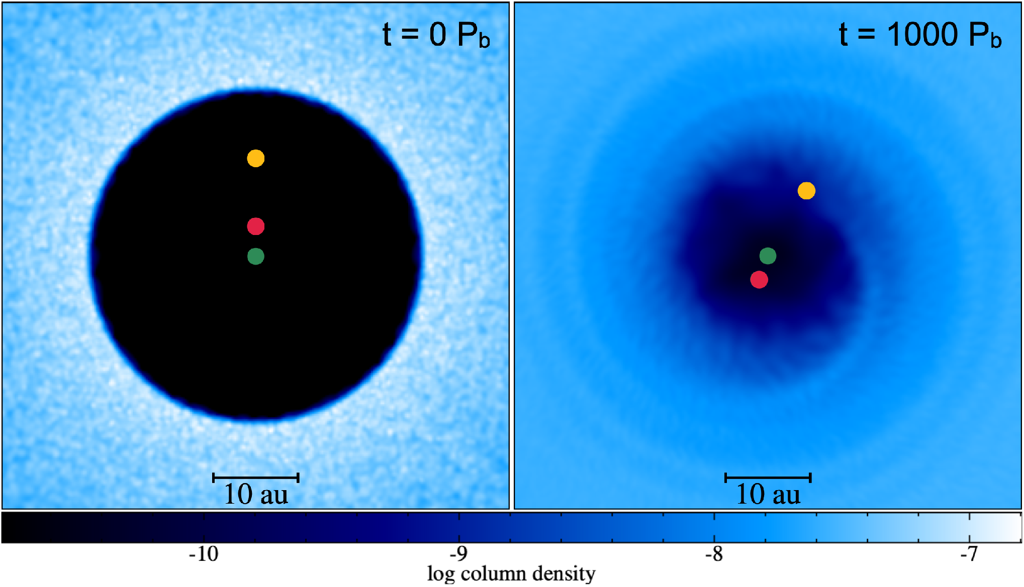
In the hydrodynamical simulations, the planets are initially interior to the initial disc edge. However, the inner edge of the disc will viscously spread inwards, eventually interacting with the planets. The left panel in Fig. 9 shows the initial setup where Pic b (yellow dot) and Pic c (red dot) are initially interior to the inner disc edge. The right panel in Fig. 9 shows the disc structure at a . At this time, the inner edge of the disc interacts with the planets.
Appendix B Planetary evolution

I examine the evolution of the two eccentric planets, Pic b and Pic c, in all hydrodynamical simulations. Fig. 10 shows the evolution of the semi-major axis (, row 1), tilt (, row 2), eccentricity (, row 3), longitude of the ascending node (, row 4), the argument of the pericentre (, row 5), and planetary mass (, row 6) as a function of time. Each column denotes a different simulation with the initial parameters given at the top of each column. The left-most column shows a simulation with no gas disc present with initial planetary tilts . The only significant difference in the planetary parameters is that there are no tilt oscillations since there is no gas disc perturbing the planetary orbits. In each case, both planets remain at nearly their initial separation from the central star. The planets undergo tilt oscillations driven by the gas disc, which are out of phase with one another. As the angular momentum of the disc increases (larger disc sizes), the tilt of the planetary orbits decreases at a slower rate as they align to the total angular momentum of the system. The eccentricities of the inner and outer planets also oscillate in time, with the amplitude of the outer planet’s eccentricity larger than the inner planet. Since the model is for a low-mass disc and the change in planetary tilt is small, the planets precess extremely slowly. However, as shown in the fifth panel, the eccentric planets undergo apsidal precession. The inner planet apsidally precesses faster than the outer planet. Finally, the masses of planets b and c increase slowly over time due to the accretion of material.