Masked Bayesian Neural Networks :
Theoretical Guarantee and its Posterior Inference

Let $\mathbb{R}$ and $\mathbb{N}$ be the sets of real numbers and natural numbers, respectively. For an integer $n\in\mathbb{N}$, we denote $[n]:=\{1,\dots,n\}$. A capital letter denotes a random variable or matrix interchangeably whenever its meaning is clear, and a vector is denoted by a bold letter, e.g. $\bm{x}:=(x_{1},\dots,x_{d})^{\top}$. For a $d$-dimensional vector $\bm{x}\in\mathbb{R}^{d}$, we denote $|\bm{x}|_{p}:=(\sum_{j=1}^{d}|x_{j}|^{p})^{1/p}$ for $1\leq p<\infty$, $|\bm{x}|_{0}:=\sum_{j=1}^{d}\mathbb{I}(x_{j}\neq 0)$ and $|\bm{x}|_{\infty}:=\max_{j\in[d]}|x_{j}|$. For a real-valued function $f:\mathcal{X}\to\mathbb{R}$ and $1\leq p<\infty$, we denote $||f||_{p,n}:=(\sum_{i=1}^{n}f(\bm{x}_{i})^{p}/n)^{1/p}$ and $||f||_{p,\mathrm{P}_{\bm{X}}}:=\left(\int_{\bm{X}\in\mathcal{X}}f(\bm{X})^{p}d\mathrm{P}_{\bm{X}}\right)^{1/p}$ where $\mathrm{P}_{\bm{X}}$ is a probability measure defined on input space $\mathcal{X}$. Moreover, we define $||f||_{\infty}=\operatorname{sup}_{\bm{x}\in\mathcal{X}}|f(\bm{x})|.$ For $b_{1}\leq b_{2}$, we define $f_{[b_{1},b_{2}]}(\cdot):=\min(\max(f(\cdot),b_{1}),b_{2})$ which is a truncated version of $f$ on $b_{1}$ and $b_{2}$. We denote $\circ$ and $\odot$ as the composition of functions and element-wise product of vectors or matrices, respectively. For a probability vector $\bm{q}\in\mathbb{R}^{r}$, we denote $\operatorname{Cat}(\bm{q})$ as the categorical distribution with the probabilities of each category being $\bm{q}$ and $\operatorname{Multi}_{\left(N,\bm{q}\right)}$ as the distribution of N many selected balls without replacement from the jar containing $r$ many balls whose selection probabilities are $\bm{q}$. For technical simplicity, we assume $\mathcal{X}=[-1,1]^{d}$.

We consider two supervised learning problems : regression and classification. In regression problems, the input vector $\bm{X}$ and the response variable $Y\in\mathbb{R}$ are generated from the model

where $\mathrm{P}_{\bm{X}}$ is the probability measure defined on $\mathcal{X}.$ Here, $f_{0}:\mathcal{X}\to\mathbb{R}$ and $\sigma_{0}^{2}>0$ are the unknown true regression function and unknown variance of the noise, respectively.

For $K$-class classification problems, the input vector $\bm{X}$ and the response variable $Y\in[K]$ are generated from the model

where $\mathrm{P}_{\bm{X}}$ is the probability measure defined on $\mathcal{X}$ and $\bm{f}_{0}:\mathcal{X}\to\mathbb{R}^{K}$ is the logit of the unknown true conditional class probability function.

For $L\in\mathbb{N}$ and $\bm{p}=(p^{(0)},p^{(1)},...,p^{(L)},p^{(L+1)})^{\top}\in\mathbb{N}^{L+2}$, DNN with the $(L,\bm{p})$ architecture is a DNN model which has $L$ hidden layers and $p^{(l)}$ many nodes at the $l$-th hidden layer for $l\in[L].$ The input and output dimensions are $p^{(0)}$ and $p^{({L+1})},$ respectively. The output of the DNN model can be written as

where $A_{l}:\mathbb{R}^{p^{(l-1)}}\mapsto\mathbb{R}^{p^{(l)}}$ for $l\in[L+1]$ is an affine map defined as $A_{l}(\bm{x}):=W_{l}\bm{x}+\bm{b}_{l}$ with $W_{l}\in\mathbb{R}^{p^{(l)}\times p^{(l-1)}}$ and $\bm{b}_{l}\in\mathbb{R}^{p^{(l)}}$ and $\rho$ is the RELU activation function. The DNN model is parameterized by $\bm{\theta}$ which is the concatenation of the weight matrices and bias vectors, that is

For a given standard DNN, the corresponding masked DNN (mDNN) is constructed by simply adding masking parameters to the standard DNN model. For $l\in[L]$, the mDNN model screens the nodes at the $l$-th hidden layer using the binary masking vector $\bm{m}^{(l)}\in\{0,1\}^{p^{(l)}}$. When $\left(\bm{m}^{(l)}\right)_{j}=0,$ the $j$-th node at the $l$-th hidden layer becomes inactive. The output of the mDNN model with the $(L,\bm{p})$ architecture can be written as

where $A_{l}$ for $l\in[L+1]$ is the affine map defined in (3) and $\rho_{\bm{m}^{(l)}}:\mathbb{R}^{p^{(l)}}\to\mathbb{R}^{p^{(l)}}$ for $l\in[L]$ is the masked-RELU activation function defined as

The model is parameterized by $\bm{M}$ and $\bm{\theta}$, where $\bm{M}\in\{0,1\}^{\sum_{l=1}^{L}p^{(l)}}$ is the concatenate of the all masking vectors

and $\bm{\theta}$ is the concatenation of the weight matrices and the bias vectors in the standard DNN model.

Note that the mDNN is nothing but a standard DNN with the architecture $(L,\tilde{\bm{p}})$ where $(\tilde{\bm{p}})_{l}=\left|\bm{m}^{(l)}\right|_{0}.$ That is, the mDNN is a reparameterization of the standard DNN using the masking vectors. This reparameterization, however, allows us to develop an efficient MCMC algorithm, in particular for searching good architectures (i.e. good masking vectors).

We adopt a data-dependent prior $\Pi_{n}$ on the parameters $\bm{M}$ and $\bm{\theta}$ (as well as $\sigma^{2}$ for regression problems). We consider a data-dependent prior to ensure the optimal posterior concentration rate and adaptiveness. We assume that a priori $\bm{M}$ and $\bm{\theta}$ (as well as $\sigma^{2}$ for regression problems) are independent.

For $\bm{M},$ we use the following hierarchical prior. For each $\bm{m}^{(l)}$ with $l\in[L]$, let $s^{(l)}:=|\bm{m}^{(l)}|_{0}$ be the sparsity of the masking vector $\bm{m}^{(l)}$. We put a prior mass on $s^{(l)}$ by

where $\lambda>0$ is a hyper-parameter. Note that the prior on $s^{(l)}$ regularizes the width of the network, and more strong regularization is enforced as more data are accumulated. Given the sparsity level $s^{(l)}$, the masking vector $\bm{m}^{(l)}$ is sampled from the set $\{\bm{m}^{(l)}\in\{0,1\}^{p^{(l)}}:|\bm{m}^{(l)}|_{0}=s^{(l)}\}$ uniformly. In other words,

and the prior of $\bm{m}^{(l)}$ is the product of (4) and (5)

For the prior of $\bm{\theta},$ we assume that

where $T:=\sum_{l=0}^{L}(p^{(l)}+1)p^{(l+1)}$ is the length of the vector $\bm{\theta},$ and choose $\mathfrak{p}$ carefully to ensure desirable theoretical properties. For high-dimensional linear regression problems, Castillo & van der Vaart 2012 and Castillo et al. 2015 notice that using a heavy-tailed distribution for the prior of the regression coefficients is essential for theoretical optimality. Motivated by these observations, we consider a heavy-tailed distribution for $\mathfrak{p}.$ Let $\mathfrak{P}$ be the class of polynomial tail distributions on $\mathbb{R}$ defined as

Examples of polynomial tail distributions are the Cauchy distribution and Student’s t-distribution. On the other hand, the Gaussian and Laplace distributions do not belong to $\mathfrak{P}.$ We assume that $\mathfrak{p}$ belongs to $\mathfrak{P}.$ We will show in Section 4 that any prior in $\mathfrak{P}$ yields the optimal posterior concentration rate.

For the prior of $\sigma^{2}$ in regression problems, a standard distribution such as the inverse-gamma distribution can be used. Any distribution whose density is positive at the true $\sigma^{2}_{0}$ works for theoretical optimality.

The idea of masking nodes in DNN has been already used in various algorithms. Dropout (Srivastava et al. 2014) and MC-dropout (Gal & Ghahramani 2016) are two representative examples, where they randomly mask the nodes of DNN during the training phase. While Dropout abolishes the masking vectors and uses the scaled-down version of the trained weights in the prediction phase, MC-dropout uses the trained weights obtained in the training phase multiplied by a random masking vectors. Since the masking vectors is treated as a random vectors following its posterior distribution at the prediction phase, our mBNN is similar to MC-dropout. A key difference between the mBNN and MC-dropout, however, is that the mBNN learns the distribution of the masking vectors from data via the posterior distribution but MC-dropout does not. That is, the mBNN learns the architecture of DNN from data, which makes the mBNN have good theoretical and empirical properties.

We consider the nonparametric regression model (1). We assume the true regression function $f_{0}$ belongs to the $\beta$-Hölder class $\mathcal{H}_{d}^{\beta}$.¹¹ 1 Theoretical results for hierarchical composition functions are provided in Appendix B. Here, the $\beta$-Hölder class $\mathcal{H}_{d}^{\beta}$ is given as

where $||f||_{\mathcal{H}^{\beta}}$ denotes the Hölder norm defined by

For inference, we consider the probabilistic model

where $f_{\bm{M},\bm{\theta}}^{\operatorname{mDNN}}(\bm{X}_{i})$ has the $(L_{n},\bm{p}_{n})$ architecture with $L_{n}$ and $\bm{p}_{n}$ given as

for positive constants $C_{L}$ and $C_{p}$ that are defined in Lemma A.1. Then, the likelihood $\mathcal{L}(w|\mathcal{D}^{(n)})$ of $w:=(\bm{M},\bm{\theta},\sigma^{2})$ is expressed as

and the corresponding posterior distribution is given as

where $\Pi_{n}$ is the prior defined on Section 3.3.

In the following theorem, we show that the mBNN model achieves the optimal (up to a logarithmic factor) posterior concentration rate to the true regression function.

The convergence rate $n^{-\beta/(2\beta+d)}$ is known to be minimax lower bound when estimating the $\beta$-Hölder smooth function (Tsybakov 2009). Our concentration rate is near optimal up to a logarithmic factor and adaptive to the smoothness of the true model.

Theoretical results for regression problem can be extended to classification problem. We consider the classification problem (2) with $K=2$, and denote $f_{0}:=\left(\bm{f}_{0}\right)_{2}-\left(\bm{f}_{0}\right)_{1}.$ We assume that $f_{0}$ belongs to the $\beta$-Hölder class $\mathcal{H}_{d}^{\beta}$. For inference, we consider the probabilistic model

where $\phi$ is the sigmoid function and $f_{\bm{M},\bm{\theta}}^{\operatorname{mDNN}}$ has the $(L_{n},\bm{p}_{n})$ architecture with $L_{n}$ and $\bm{p}_{n}$ given as (7) and (8). Then, the likelihood $\mathcal{L}(w|\mathcal{D}^{(n)})$ of $w:=(\bm{M},\bm{\theta})$ is expressed as

In the following theorem, we prove that the mBNN model achieves the optimal (up to a logarithmic factor) posterior concentration rate to the true conditional class probability adaptive to the smoothness of the true model.

Not only the fast concentration rate, the mBNN achieves the optimal sparsity too. Theorem 4.3, which is a by-product of the proofs for Theorems 4.1 and 4.2, gives the level of sparsity of the mBNN.

Yarotsky 2017 proves that the lower bound of the sparsity of DNNs to approximate functions in $\mathcal{H}_{d}^{\beta}$ is equal to $\mathfrak{s}_{n}$ up to a logarithmic factor. That is, the mBNN automatically learns the optimal sparsity from data.

The proposed MCMC algorithm samples $\bm{\theta}$ (and $\sigma^{2}$) given $\bm{M}$ and $\mathcal{D}^{(n)}$ and then samples $\bm{M}$ given $\bm{\theta}$ (and $\sigma^{2}$) and $\mathcal{D}^{(n)}$, and iterates these two samplings until convergence.

There are various efficient sampling algorithms for $\bm{\theta}$ (and $\sigma^{2}$) given $\bm{M}$ and $\mathcal{D}^{(n)}$ such as Hamiltonian Monte Carlo (HMC) (Neal et al. 2011), Stochastic Gradient Langevin Dynamics (SGLD) (Welling & Teh 2011) and Stochastic Gradient HMC (SGHMC) (Chen et al. 2014). In practice, we select a sampling algorithm among those depending on the sizes of data and model.

For generating $\bm{M}$ from its conditional posterior, we consider the Metropolis-Hastings (MH) algorithm. The hardest part is to design a good proposal distribution since the dimension of $\bm{M}$ is quite large and all entries are binary. In the next subsection, we propose an efficient proposal distribution for $\bm{M}.$

Essentially, sampling $\bm{M}$ is equivalent to sampling a large dimensional binary vector. A well known strategy for sampling a large dimensional binary vector is to use the MH algorithm with the locally informed proposal (Umrigar 1993; Zanella 2020) given as

where $l(\bm{M})$ is the log-posterior of $\bm{M}$ and $H(\bm{M})$ is the Hamming ball of a certain size around $\bm{M}$. The key point of (9) is to give more probability to $\bm{M}^{\star}$ whose posterior probability is high. While powerful, this locally informed proposal requires to compute $l(\bm{M}^{\star})$ for every $\bm{M}^{\star}\in H(\bm{M}),$ which is time consuming. To resolve this problem, we propose a proposal distribution which only uses the information of the current $\bm{M}$.

First, we select either birth or death, where birth makes some inactive nodes become active and death makes some active nodes become inactive. When death is selected, motivated by the pruning algorithms (Lee et al. 2018; Tanaka et al. 2020), our strategy is to prune less sensitive nodes. That is, we delete nodes which do not affect much to the current DNN model when their values are changed. On the other hand, when birth is selected, we choose some of inactive nodes with equal probabilities and make them active. We use equal probabilities because the posterior of the edges connected to the inactive nodes is the same as the prior and thus there is no reason to prefer certain inactive nodes more. Moreover, the proposal with equal probabilities for birth is helpful for increasing the acceptance rate of death to result in fast mixing.

To be more specific, we first select the move $u\in\{0,1\}$ with probability 1/2, where $u=0$ and $u=1$ indicates birth and death, respectively. In addition, we select an inteager $N$ from $[N_{\max}]$ uniformly, where $N_{\max}$ is a prespecified positive integer. Then, we select randomly $N$ nodes among the nodes whose masking values are $u$ following $\operatorname{Multi}_{\left(N,\bm{Q}_{u}\right)}$, where

Even though $l(\bm{M})$ is defined only on binary vectors, the gradient $\nabla l(\bm{M})=\partial l(\bm{M})/\partial\bm{M}$ of $l(\bm{M})$ can be defined by extending the domain of $l(\bm{M})$ appropriately. Finally, we flip the masking values of the selected nodes to have a new proposal $\bm{M}^{*}.$ To sum up, the proposal distribution first selects a set of nodes $\{i_{1},\dots,i_{N}\}$ following $\operatorname{Multi}_{\left(N,\bm{Q}_{u}\right)}$ and changes their mask values to $(1-\bm{M}_{i_{1}},\dots,1-\bm{M}_{i_{N}})$. Then, we accept the new proposal $\bm{M}^{*}$ with probability

where

and $\bm{Q}^{\star}_{1-u}$ is the selection probability vector defined by (10) or (11) with the mask vectors $\bm{M}^{\star}.$ Note that some inactive nodes become active when $u=0$ (i.e. birth of nodes) and some active nodes become inactive when $u=1$ (i.e. death of nodes). The proposed MH algorithm is summarized in Algorithm 1.

One may consider a linear approximation of $l$ in (9) using the gradient information at $\bm{M}$, as is suggested by Grathwohl et al. 2021 and Zhang et al. 2022. However, we found that the linear approximation is not accurate for the mBNN, which is partly because the corresponding DNN is not locally smooth enough. In section 6.5, we provide the results of the experiment for comparing several proposal distributions which support the choice of (10) and (11).

We obtain the predictive distribution when the true regression function is the noisy polynomial regression problem considered in Hernández-Lobato & Adams 2015. Inputs $x_{i}$ are sampled from $x_{i}\sim\operatorname{Uniform}(-4,4)$ and the corresponding outputs $y_{i}$ are obtained by $y_{i}=x_{i}^{3}+\epsilon_{i}$, where $\epsilon_{i}\sim N(0,9)$. We generate 20 training examples and compare the predictive distribution of the mBNN with that of BNN by generating 1000 MCMC samples from each model. For each model, the two hidden layer MLP with the layer sizes (1000,1000) is used.

The mean and 95% predictive intervals of the predictive distributions of BNN and the mBNN are presented in Figure 1. The figure illustrates that BNN quantifies uncertainty on a data sparse region overly to have a too wide predictive interval. Note that the true regression function is assumed to smooth and hence it is possible to transfer information on data dense regions to data sparse regions. Thus, proper uncertainty quantification even on data sparse regions could be possible. The coverage probability of the predictive interval of the mBNN is 95.3%, which is obtained by generating additional 1000 test sample, while that of BNN is 98.6%. The results indicate that deleting unnecessary nodes is important not only for fast convergence rates but also proper uncertainty quantification.

We evaluate BNN, node-sparse VI (NS-VI) (Louizos et al. 2017) and the mBNN on four UCI regression datasets (Boston, Concrete, Energy, Yacht). For each dataset, we construct 20 random 90-to-10 train-test splits to provide the standard errors. For each method, the two hidden layer MLP with the layer sizes (1000,1000) is used. We select 20 models from several thousands MCMC samples and compare the predictive distributions obtained by the selected 20 models in terms of generalization and uncertainty quantification.

In Table 1, we report the means and standard errors of the performance measures on the 20 repeated experiments. For the performance measures, the coverage probability of the 95% predictive interval (Coverage), the root mean square error (RMSE) of the Bayes estimator, the negative log-likelihood (NLL) and continuous ranked probability score (CRPS) (Gneiting & Raftery 2007) on test data are considered.

It is obvious that the mBNN outperform the other two competitors with respect to all of the four measures. That is, the mBNN is good at not only estimating the regression function and but also uncertainty quantification. It is noticeable that NS-VI performs too badly, which suggests that full Bayesian analysis of DNN is must. More detailed results such as the sparsity and the sensitivity to the hyper-parameter selection are provided in Appendix E.

Bayesian structural time series (BSTS) models (Scott & Varian 2014; Qiu et al. 2018) provide a useful tool for time series forecasting, nowcasting, inferring causal relationships and anomaly detection (Brodersen et al. 2015; Feng & Tian 2021). The key of BSTS is the state space model, which is given as

where $\bm{x}_{t}\in\mathbb{R}^{d}$, $y_{t}\in\mathbb{R}$ and $\mu_{t}\in\mathbb{R}$ denote observed input variables, output variable and unobserved local trend at time $t$, respectively. For inference and prediction, MCMC algorithm using Kalman filter (Welch et al. 1995; Durbin & Koopman 2002) is mainly used.

In many cases, the linear component $\bm{\beta}^{\top}\bm{x}_{t}$ may not be insufficient to explain complicate relations between inputs and outputs, and DNN can be considered instead. In turn, the mBNN is a useful inferential tool for this nonlinear BSTS. To illustrate that the mBNN works well for BSTS, we analyze a real dataset consisting of daily search volumes of several keywords collected by a Korea search platform company. The dataset consists of daily search volumes of keywords in year 2021 associated with a pre-specified product (eg. shampoo). The aim is to predict the search volume of the pre-specified product based on the search volumes of other related keywords.

We apply the three BSTS models corresponding to the three regression components - linear, BNN and the mBNN. For BNN and the mBNN, the two hidden layer MLP with the layer sizes (100,100) is used. The predictive intervals with the NLL and RMSE values on the data from $t=241$ to $t=365$ obtained by the posterior distribution inferred on the data from $t=1$ to $t=240$ are presented in figure 2. It is clearly observed that the mBNN is superior in both nowcasting ability and uncertainty quantification. It is interesting that the predictive intervals of the linear and BNN models are much wider than those of the mBNN, which amply indicates that the choice of an appropriate architecture of DNN is crucial for desirable uncertainty quantification. More details about the dataset, methodology and additional experimental results are provided in Appendix D.3.

We also extend the mBNN to masked Bayesian convolution neural network (mBCNN) for image dataset. We construct a masked CNN (mCNN) by adding masking vectors to the CNN model. See Appendix C.2 for details of the mBCNN.

We evaluate compression ability of the mBCNN on image datasets. For comparison, we use node-sparse versions of approximated Bayesian methodologies : NS-VI, node-sparse Deep ensemble (NS-Ens) and node-sparse MC-dropout (NS-MC). Detail description of competitors are provided in Appendix D.4. For each methods, ResNet18 (He et al. 2016) architecture is used. For fair comparison, we use five networks for inference in all the methods. We repeat the experiments 3 times with different seeds.

In Table 2, we report the means and standard errors of the performance measures on the repeated experiments. For the performance measures, accuracy of the Bayes estimator, NLL, expected calibration error (ECE) (Kumar et al. 2019) of test data are considered. In addition, we report inferential costs (FLOPs) and the numbers of nonzero parameters (Capacity) relative to the non-sparse model. The results in Table 2 show that mBCNN provides better generalization and uncertainty quantification with less inferential cost and model capacity compared to the other competitors. That is, the mBNN is a useful tool for compressing complex DNNs without hampering uncertainty quantification much.

To illustrate the efficiency of our proposal distribution in Algorithm 1, we conduct a comparative experiment. As an alternative to the proposal distribution with selection probability (10) for birth and (11) for death, we consider the following candidates for the selection probability of either birth or death:

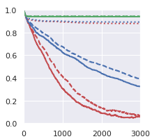
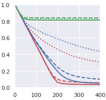
While (13) gives the same selection probability on each active (or inactive) node, (14) and (15) put proposals depending on the role of each node. The proposal of (14) is devised to select less sensitive nodes more by giving proposal probabilities reciprocally proportional to $|\nabla l(\bm{M})|$, and (15) uses a linear approximation of $l$ in (9) (Grathwohl et al. 2021).

We compare the speeds of convergence of the MCMC algorithm with the 9 proposal distributions which are all $3^{2}$ combinations of the three candidates (13), (14) and (15) and the two moves for birth and death. Figure 3 presents how the ratios of the activated nodes relative to the largest DNN decrease in the burn-in phase of the MCMC algorithm. It is obvious that our proposal (the red solid lines) is most fast to eliminate unnecessary nodes. Note that the proposals involving the linear approximation of $l(\bm{M})$ do not work well, which suggests that DNNs are not smooth enough to be approximated linearly.

References

- Bai et al. (2020) Bai, J., Song, Q., and Cheng, G. Efficient variational inference for sparse deep learning with theoretical guarantee. Advances in Neural Information Processing Systems, 33:466–476, 2020.
- Banbura et al. (2010) Banbura, M., Giannone, D., and Reichlin, L. Nowcasting. 2010.
- Brodersen et al. (2015) Brodersen, K. H., Gallusser, F., Koehler, J., Remy, N., and Scott, S. L. Inferring causal impact using bayesian structural time-series models. The Annals of Applied Statistics, pp. 247–274, 2015.
- Castillo & van der Vaart (2012) Castillo, I. and van der Vaart, A. Needles and straw in a haystack: Posterior concentration for possibly sparse sequences. The Annals of Statistics, 40(4):2069–2101, 2012.
- Castillo et al. (2015) Castillo, I., Schmidt-Hieber, J., and Van der Vaart, A. Bayesian linear regression with sparse priors. The Annals of Statistics, 43(5):1986–2018, 2015.
- Chen et al. (2014) Chen, T., Fox, E., and Guestrin, C. Stochastic gradient hamiltonian monte carlo. In International conference on machine learning, pp. 1683–1691. PMLR, 2014.
- Chérief-Abdellatif (2020) Chérief-Abdellatif, B.-E. Convergence rates of variational inference in sparse deep learning. In International Conference on Machine Learning, pp. 1831–1842. PMLR, 2020.
- Chin et al. (2020) Chin, T.-W., Ding, R., Zhang, C., and Marculescu, D. Towards efficient model compression via learned global ranking. In Proceedings of the IEEE/CVF conference on computer vision and pattern recognition, pp. 1518–1528, 2020.
- Cranmer et al. (2021) Cranmer, M., Tamayo, D., Rein, H., Battaglia, P., Hadden, S., Armitage, P. J., Ho, S., and Spergel, D. N. A bayesian neural network predicts the dissolution of compact planetary systems. Proceedings of the National Academy of Sciences, 118(40), 2021.
- Deng et al. (2019) Deng, W., Zhang, X., Liang, F., and Lin, G. An adaptive empirical bayesian method for sparse deep learning. Advances in neural information processing systems, 2019:5563, 2019.
- Durbin & Koopman (2002) Durbin, J. and Koopman, S. J. A simple and efficient simulation smoother for state space time series analysis. Biometrika, 89(3):603–616, 2002.
- Feng & Tian (2021) Feng, C. and Tian, P. Time series anomaly detection for cyber-physical systems via neural system identification and bayesian filtering. In Proceedings of the 27th ACM SIGKDD Conference on Knowledge Discovery & Data Mining, pp. 2858–2867, 2021.
- Filos et al. (2019) Filos, A., Farquhar, S., Gomez, A. N., Rudner, T. G., Kenton, Z., Smith, L., Alizadeh, M., De Kroon, A., and Gal, Y. A systematic comparison of bayesian deep learning robustness in diabetic retinopathy tasks. arXiv preprint arXiv:1912.10481, 2019.
- Frankle & Carbin (2018) Frankle, J. and Carbin, M. The lottery ticket hypothesis: Finding sparse, trainable neural networks. In International Conference on Learning Representations, 2018.
- Gal & Ghahramani (2016) Gal, Y. and Ghahramani, Z. Dropout as a bayesian approximation: Representing model uncertainty in deep learning. In international conference on machine learning, pp. 1050–1059. PMLR, 2016.
- Gan et al. (2015) Gan, Z., Chen, C., Henao, R., Carlson, D., and Carin, L. Scalable deep poisson factor analysis for topic modeling. In International Conference on Machine Learning, pp. 1823–1832. PMLR, 2015.
- Ghosal & Van Der Vaart (2007) Ghosal, S. and Van Der Vaart, A. Convergence rates of posterior distributions for noniid observations. The Annals of Statistics, 35(1):192–223, 2007.
- Ghosh et al. (2019) Ghosh, S., Yao, J., and Doshi-Velez, F. Model selection in bayesian neural networks via horseshoe priors. J. Mach. Learn. Res., 20(182):1–46, 2019.
- Giannone et al. (2008) Giannone, D., Reichlin, L., and Small, D. Nowcasting: The real-time informational content of macroeconomic data. Journal of monetary economics, 55(4):665–676, 2008.
- Gneiting & Raftery (2007) Gneiting, T. and Raftery, A. E. Strictly proper scoring rules, prediction, and estimation. Journal of the American statistical Association, 102(477):359–378, 2007.
- Gomez et al. (2019) Gomez, A. N., Zhang, I., Kamalakara, S. R., Madaan, D., Swersky, K., Gal, Y., and Hinton, G. E. Learning sparse networks using targeted dropout. arXiv preprint arXiv:1905.13678, 2019.
- Grathwohl et al. (2021) Grathwohl, W., Swersky, K., Hashemi, M., Duvenaud, D., and Maddison, C. Oops i took a gradient: Scalable sampling for discrete distributions. In International Conference on Machine Learning, pp. 3831–3841. PMLR, 2021.
- Györfi et al. (2002) Györfi, L., Kohler, M., Krzyżak, A., and Walk, H. A distribution-free theory of nonparametric regression, volume 1. Springer, 2002.
- Han et al. (2015) Han, S., Pool, J., Tran, J., and Dally, W. Learning both weights and connections for efficient neural network. Advances in neural information processing systems, 28, 2015.
- Harvey et al. (2017) Harvey, N., Liaw, C., and Mehrabian, A. Nearly-tight vc-dimension bounds for piecewise linear neural networks. In Conference on learning theory, pp. 1064–1068. PMLR, 2017.
- He et al. (2016) He, K., Zhang, X., Ren, S., and Sun, J. Deep residual learning for image recognition. In Proceedings of the IEEE conference on computer vision and pattern recognition, pp. 770–778, 2016.
- He et al. (2017) He, Y., Zhang, X., and Sun, J. Channel pruning for accelerating very deep neural networks. In Proceedings of the IEEE international conference on computer vision, pp. 1389–1397, 2017.
- Hernández-Lobato & Adams (2015) Hernández-Lobato, J. M. and Adams, R. Probabilistic backpropagation for scalable learning of bayesian neural networks. In International conference on machine learning, pp. 1861–1869. PMLR, 2015.
- Hoffman et al. (2014) Hoffman, M. D., Gelman, A., et al. The no-u-turn sampler: adaptively setting path lengths in hamiltonian monte carlo. J. Mach. Learn. Res., 15(1):1593–1623, 2014.
- Izmailov et al. (2021) Izmailov, P., Vikram, S., Hoffman, M. D., and Wilson, A. G. G. What are bayesian neural network posteriors really like? In International Conference on Machine Learning, pp. 4629–4640. PMLR, 2021.
- Jantre et al. (2021) Jantre, S., Bhattacharya, S., and Maiti, T. Layer adaptive node selection in bayesian neural networks: Statistical guarantees and implementation details. arXiv preprint arXiv:2108.11000, 2021.
- Kingma & Ba (2014) Kingma, D. P. and Ba, J. Adam: A method for stochastic optimization. arXiv preprint arXiv:1412.6980, 2014.
- Kingma et al. (2015) Kingma, D. P., Salimans, T., and Welling, M. Variational dropout and the local reparameterization trick. Advances in neural information processing systems, 28:2575–2583, 2015.
- Kohler & Langer (2021) Kohler, M. and Langer, S. On the rate of convergence of fully connected deep neural network regression estimates. The Annals of Statistics, 49(4):2231–2249, 2021.
- Kumar et al. (2019) Kumar, A., Liang, P. S., and Ma, T. Verified uncertainty calibration. Advances in Neural Information Processing Systems, 32, 2019.
- Lakshminarayanan et al. (2017) Lakshminarayanan, B., Pritzel, A., and Blundell, C. Simple and scalable predictive uncertainty estimation using deep ensembles. Advances in neural information processing systems, 30, 2017.
- Lee & Lee (2022) Lee, K. and Lee, J. Asymptotic properties for bayesian neural network in besov space. In Advances in Neural Information Processing Systems, 2022. URL https://openreview.net/forum?id=y5ziOXtKybL.
- Lee et al. (2018) Lee, N., Ajanthan, T., and Torr, P. Snip: Single-shot network pruning based on connection sensitivity. In International Conference on Learning Representations, 2018.
- Louizos et al. (2017) Louizos, C., Ullrich, K., and Welling, M. Bayesian compression for deep learning. Advances in neural information processing systems, 30, 2017.
- MacKay (1992) MacKay, D. J. A practical bayesian framework for backpropagation networks. Neural computation, 4(3):448–472, 1992.
- Molchanov et al. (2017) Molchanov, D., Ashukha, A., and Vetrov, D. Variational dropout sparsifies deep neural networks. In International Conference on Machine Learning, pp. 2498–2507. PMLR, 2017.
- Nalisnick et al. (2019) Nalisnick, E., Hernández-Lobato, J. M., and Smyth, P. Dropout as a structured shrinkage prior. In International Conference on Machine Learning, pp. 4712–4722. PMLR, 2019.
- Neal (2012) Neal, R. M. Bayesian learning for neural networks, volume 118. Springer Science & Business Media, 2012.
- Neal et al. (2011) Neal, R. M. et al. Mcmc using hamiltonian dynamics. Handbook of markov chain monte carlo, 2(11):2, 2011.
- Polson & Ročková (2018) Polson, N. G. and Ročková, V. Posterior concentration for sparse deep learning. In Proceedings of the 32nd International Conference on Neural Information Processing Systems, pp. 938–949, 2018.
- Qiu et al. (2018) Qiu, J., Jammalamadaka, S. R., and Ning, N. Multivariate bayesian structural time series model. J. Mach. Learn. Res., 19(1):2744–2776, 2018.
- Schmidt-Hieber (2020) Schmidt-Hieber, J. Nonparametric regression using deep neural networks with relu activation function. The Annals of Statistics, 48(4):1875–1897, 2020.
- Scott & Varian (2014) Scott, S. L. and Varian, H. R. Predicting the present with bayesian structural time series. International Journal of Mathematical Modelling and Numerical Optimisation, 5(1-2):4–23, 2014.
- Shin et al. (2021) Shin, M., Cho, H., Min, H.-s., and Lim, S. Neural bootstrapper. Advances in Neural Information Processing Systems, 34:16596–16609, 2021.
- Srivastava et al. (2014) Srivastava, N., Hinton, G., Krizhevsky, A., Sutskever, I., and Salakhutdinov, R. Dropout: a simple way to prevent neural networks from overfitting. The journal of machine learning research, 15(1):1929–1958, 2014.
- Tanaka et al. (2020) Tanaka, H., Kunin, D., Yamins, D. L., and Ganguli, S. Pruning neural networks without any data by iteratively conserving synaptic flow. Advances in Neural Information Processing Systems, 33:6377–6389, 2020.
- Tsybakov (2009) Tsybakov, A. B. Introduction to nonparametric estimation, 2009.
- Umrigar (1993) Umrigar, C. Accelerated metropolis method. Physical review letters, 71(3):408, 1993.
- van der Vaart & van Zanten (2008) van der Vaart, A. W. and van Zanten, J. H. Rates of contraction of posterior distributions based on gaussian process priors. The Annals of Statistics, 36(3):1435–1463, 2008.
- Wang et al. (2019) Wang, C., Grosse, R., Fidler, S., and Zhang, G. Eigendamage: Structured pruning in the kronecker-factored eigenbasis. In International Conference on Machine Learning, pp. 6566–6575. PMLR, 2019.
- Wang et al. (2015) Wang, H., Wang, N., and Yeung, D.-Y. Collaborative deep learning for recommender systems. In Proceedings of the 21th ACM SIGKDD international conference on knowledge discovery and data mining, pp. 1235–1244, 2015.
- Wang et al. (2021) Wang, Y., Deng, W., and Lin, G. Bayesian sparse learning with preconditioned stochastic gradient mcmc and its applications. Journal of Computational Physics, 432:110134, 2021.
- Welch et al. (1995) Welch, G., Bishop, G., et al. An introduction to the kalman filter. 1995.
- Welling & Teh (2011) Welling, M. and Teh, Y. W. Bayesian learning via stochastic gradient langevin dynamics. In Proceedings of the 28th international conference on machine learning (ICML-11), pp. 681–688. Citeseer, 2011.
- Wen et al. (2016) Wen, W., Wu, C., Wang, Y., Chen, Y., and Li, H. Learning structured sparsity in deep neural networks. Advances in neural information processing systems, 29:2074–2082, 2016.
- Wenzel et al. (2020) Wenzel, F., Roth, K., Veeling, B., Swiatkowski, J., Tran, L., Mandt, S., Snoek, J., Salimans, T., Jenatton, R., and Nowozin, S. How good is the bayes posterior in deep neural networks really? In International Conference on Machine Learning, pp. 10248–10259. PMLR, 2020.
- Wilson & Izmailov (2020) Wilson, A. G. and Izmailov, P. Bayesian deep learning and a probabilistic perspective of generalization. Advances in neural information processing systems, 33:4697–4708, 2020.
- Wu et al. (2022) Wu, T.-Y., Rachel Wang, Y., and Wong, W. H. Mini-batch metropolis–hastings with reversible sgld proposal. Journal of the American Statistical Association, 117(537):386–394, 2022.
- Xie & Xu (2020) Xie, F. and Xu, Y. Adaptive bayesian nonparametric regression using a kernel mixture of polynomials with application to partial linear models. Bayesian Analysis, 15(1):159–186, 2020.
- Yarotsky (2017) Yarotsky, D. Error bounds for approximations with deep relu networks. Neural Networks, 94:103–114, 2017.
- Zanella (2020) Zanella, G. Informed proposals for local mcmc in discrete spaces. Journal of the American Statistical Association, 115(530):852–865, 2020.
- Zhang et al. (2019) Zhang, R., Li, C., Zhang, J., Chen, C., and Wilson, A. G. Cyclical stochastic gradient mcmc for bayesian deep learning. In International Conference on Learning Representations, 2019.
- Zhang et al. (2020) Zhang, R., Cooper, A. F., and De Sa, C. M. Asymptotically optimal exact minibatch metropolis-hastings. Advances in Neural Information Processing Systems, 33:19500–19510, 2020.
- Zhang et al. (2022) Zhang, R., Liu, X., and Liu, Q. A langevin-like sampler for discrete distributions. In International Conference on Machine Learning, pp. 26375–26396. PMLR, 2022.
Appendix A Proofs for Main Theorems
A.1 Additional notations
In this section, we describe additional notations not mentioned earlier.
We define as the function class of truncated DNNs with architecture :
In a similar fashion, we define as the function class of truncated mDNNs with architecture :
and as
For a real number , we denote . For a vector and dimensional index vector , we denote as the sub-vector whose elements are consist of th index of . Let , . For a real-valued function and , we denote and where is a probability measure defined on input space .
For two positive sequences and , we denote if there exists a positive sequence such that for all . We denote if and hold. We use the little notation, that is, we write if .
Let be a set of functions and be a semimetric defined on . We denote and as the -covering number and -packing number of w.r.t. , respectively. Also, we denote as the VC dimension of the set .
A.2 Auxiliary lemmas
First, we describe a lemma that approximates Hölder smooth functions as DNN functions.
Lemma A.1 (Theorem 2 of Kohler & Langer 2021).
There exists and only depending on such that for every with , there exist with