Detection of Non-uniformity in Parameters for Magnetic Domain Pattern Generation by Machine LearningPreprint: AON/050511
Abstract
We estimate the spatial distribution of heterogeneous physical parameters involved in the formation of magnetic domain patterns of polycrystalline thin films by using convolutional neural networks. We propose a method to obtain a spatial map of physical parameters by estimating the parameters from patterns within a small subregion window of the full magnetic domain and subsequently shifting this window. To enhance the accuracy of parameter estimation in such subregions, we employ large-scale models utilized for natural image classification and exploit the benefits of pretraining. Using a model with high estimation accuracy on these subregions, we conduct inference on simulation data featuring spatially varying parameters and demonstrate the capability to detect such parameter variations.
I Introduction
Magnetic thin films are utilized in recordingmagnetic_media1; magnetic_media2 media such as magnetic tapes and hard disks, as well as in optical insulatorsmurayama2006nanoscale; 502265 and switching elementsalbert2000spin; sato2001fecobn. Advancements in these technologies can be expected by controlling the properties of magnetic thin films. However, various factors are associated with these properties, including the type and ratio of elements, temperature, and pressure during the manufacturing process. It is difficult to determine the conditions producing magnetic thin films with the desired properties, and hence, progress has relied on the experimenter’s empirical rules and trial and error.
Against this background, research aimed at using machine learning to assist in the creation of magnetic thin films with desired properties has been progressing. For instance, methods have been tried that directly optimize the fabrication conditions using Bayesian optimizationdoi:10.1063/1.5123019doi:10.1080/27660400.2022.2094698 or reinforcement learningTran:22, and there are techniques that accelerate screening by estimating difficult-to-measure properties of thin films from relatively easily measurable features, such as material element ratiosarticle331851690 and demagnetization curvesDENGINA2022114797.
In recent years, attempts have been made to estimate difficult-to-measure physical parameters of thin films from magnetic domain pattern images. Various methods have been employed for this purpose, including topological data analysis article_persistenthomology, convolutional neural networks (CNN) article_348428914; 10.1038/s41524-020-00485-2, and statistical metrics based on human visual cognition doi:10.7566/JPSJ.90.044705. These methods have been used to estimate physical parameters related to magnetic domain pattern generation and have enabled quantitative evaluations of labyrinthine and island structures. Specifically, the use of CNNs has yielded notable results. For instance, our research group article_348428914 successfully estimated the anisotropy parameter in the time-dependent Ginzburg-Landau equation, while Kawaguchi et al. 10.1038/s41524-020-00485-2 estimated the Dzyaloshinskii-Moriya parameter and magnetic anisotropy dispersion in the Landau-Lifshitz-Gilbert equation from simulation data. Additionally, Kawaguchi et al. successed in estimating the Dzyaloshinskii-Moriya parameter from actual data.
Investigations utilizing machine learning to estimate parameters of magnetic domain patterns typically employ artificial magnetic domain patterns synthesized by micromagnetic simulations, as training data for machine learning models. Micromagnetic simulations reproduce the microscale behaviors of magnetic materials. Factors at the mesoscale, such as crystal size, composition at the grain boundaries, and particle orientation, have been noted to exert a tangible influence upon macroscopic magnetism, rendering micromagnetic simulations a potentially vital contribution to the comprehension and development of magnetic materials. Furthermore, given the existence of real samples where these mesostructures are not spatially homogeneous, there is significance in estimating parameters that are spatially dependent. The magnetic domain patterns synthesized via micromagnetic simulations has been confirmed to resemble those within actual materials possessing analogous parametersNakatani_1989. Additionally, micromagnetic simulations are capable of replicating memory effects and topological melting effects in the formation process of real magnetic domain patterns PhysRevE.70.046204, thereby providing a compelling rationale for considering magnetic domain patterns synthesized by micromagnetic simulations as meaningful training data for machine learning models.
In this study, we estimate the spatial distribution of non-uniform physical parameters for the analysis of polycrystalline thin films by using a CNN. For the entire magnetic domain pattern, we estimated the physical parameters from patterns within a small subregion of the window and estimate the spatial distribution of physical parameters by shifting this window. Our previous research showed that the accuracy of parameter estimation deteriorates when the pattern area is small. Here, we significantly improve the estimation accuracy of the estimation from small subregion patterns compared with the preceding model and achieved the above objective through the following methods:
- •
Large-scale models - Large-scale models have many model parameters. Although they require larger computational resources and are more prone to overfitting when training data is scarce, they can handle more complex data if sufficient training data is available.
- •
Pretraining - Pretrainingpan2009survey; 9134370, also referred to as transfer learning, involves initially training the model on data from a different domain before training it on the target domain data. This accelerates learning and prevents overfitting for models with many parameters. Pretraining is particularly useful when the cost of obtaining target domain data is high. Pretraining is often done on ImageNetdeng2009imagenet, which is a dataset of natural images used for image classification. Pretraining with ImageNet has also been applied in medical research, such as for CTdoi:10.1148/ryai.2019180066 and ultrasoundcancers13040738 images, as well as in material science for predicting the physical properties of magnets 8955506 and classifying defects in metal materials pretrained_cnn_defects.
The previous research by Kawaguchi et al.10.1038/s41524-020-00485-2 and our own workarticle_348428914 used small-scale CNN models designed without pretraining. In this study, we examined the usefulness of large-scale CNN models and pretraining in predicting the properties of magnetic thin films and obtained positive results. Our contributions are as follows:
- •
We performed inference on test data with spatially varying parameters and demonstrated that we could detect changes in those parameters.
- •
We showed that large-scale models, which are designed for natural image classification, are effective for estimating small-region simulation parameters, and that pretraining with natural images is useful.
This paper is organized as follows. Sect.II gives an overview of teh numerical experiments. Sect.II.2 explains the simulation model used to generate the magnetic domain pattern data. Sect.II.3.2 describes the machine-learning model that we developed to analyze the magnetic domain patterns. Sect III evaluates the effectiveness of our model by verifying if the learning model can correctly infer the parameter changes. Sect.IV presents the results and discussion of each numerical experiment. Sect.V concludes this paper.
II numerical experiments
II.1 Overview of Numerical Experiments
The numerical experiments conducted in this study are composed of two sequential experiments, as depicted in Fig. 1. Experiment I utilizes data obtained from simulations that were executed with spatially uniform parameters, and it aims to train the model to estimate parameters, noise coefficient and the exchange interaciton coefficient described in Sect. IIB. Experiment II employs the machine learning model trained in Experiment I. The machine learning model infers the spatial distribution of and based on data from simulations in which was spatially varied while was fixed. Experiment II aims to investigate wheter the machine learning model can detect spatial change in simulation parameter and, even in the presence of such spatial variations in parameter , wheter it can reliably infer the fixed parameter .

The flow chart depicts the outline of two sequential experiments. Experiment I is for training and model selection. Experiment II is for inference of spatial distribution of parameters with the machine learning model trained in Experiment I.
II.2 Simulation and Magnetic Domain Pattern Acquisition
We modeled the average value of the -component of the spin in a small area at on a magnetic thin film placed on the xy plane as and simulated the hysteresis process of the thin film by using time dependent Ginzburg-Landau10.1103/physrevb.72.094406 equation
| (1) |
Here, is the time-dependent external magnetic field, is the magnetic anisotropy coefficient, is spatially independent and time-invariant noise following a standard normal distribution, is the noise coefficient, is the dipole interaction coefficient, and is the exchange interaction coefficient. We initialized with random values from a uniform distribution . The time step width was set to 0.1.
The external magnetic field was varied according to the following equation.
| (2) |
Here, is the maximum value of the external magnetic field during the hysteresis process. In this setting, the change in the external magnetic field is very slow compared with the change in Eq. 1.; thus, Eq. 1 can always be considered as representing a stationary state. Under the conditions, the hysteresis process shows a closed hysteresis loop, as shown in Fig. 2.
II.2.1 Generation of spatially uniform data
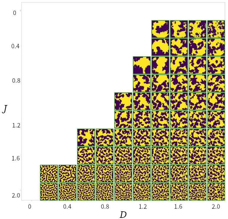
In the simulation, the space was discretized into pixels, and periodic conditions were set. To obtain a variety of hysteresis processes, we conducted simulations with different values of and . We fixed the other parameters , and , as in the previous research10.1103/physrevb.72.094406. We varied both and in the range from 0.1 to 2.0 in steps of 0.1. When both and were small, the calculation became unstable, so we excluded such combinations from the datasets. The combinations of and in the dataset are listed in the Appendix.
In the hysteresis process illustrated in Fig. 2, the magnetic domain pattern utilized for machine learning was acquired at the moment the average value of throughout the entire system attained zero for a second time following its initial time. The values of tend to approximate either +1 or -1. The values of are binarized to take either +1 or -1 with a threshold of 0. Examples of the obtained magnetic domain patterns are shown in Figs. 3 and 4.

A representative example of the hysteresis simulation used in this study. The vertical axis represents the average value of magnetization () of the entire system at each time step, and the horizontal axis represents the external magnetic field (). The initial state is at the origin, and the time evolution is shown by the black arrows. The magnetic domain pattern at the point where the average magnetization becomes zero for the second time, indicated by the red star, was used to estimate the simulation parameters.

We performed 12 simulations with random seeds for the initial values, where , for each combination of and and created a dataset.
II.2.2 Generation of Spatially Inhomogeneous Data
We conducted an numerical experiment to confirm whether the model learned with the data collected in II.2 could detect changes in the parameter from domain patterns generated from simulations with spatially varying . We discretized the simulation space into pixels, set periodic boundary conditions, and called the region within 192 pixels from the boundary the outer, and the rest the inner. We fixed the value of in the outer at 1.0 and changed the value of in the inner from 0.1 to 1.9 in increments of 0.3, and performed the hysteresis process simulations. We refer to the value of in the inner . The other parameters were fixed . Fig. 5 shows a schematic diagram of the spatial variation in .
As described in Sect.II.2.1, we obtained magnetic domain patterns in the hysteresis process with an average magnetization of zero under these conditions. Examples of these magnetic domain patterns are shown in Fig. 6.

Magnetic domain patterns were generated in the simulation by varying the value of in the inner region () and fixing the value in the outer region to . We determined whether the value of can be estimated from the magnetic domain patterns within a sliding window defined by Algorithm 1 and whether this change in could be detected.

Examples of magnetic domain patterns found by varying in the inner region and setting in the outer region. The image’s side length is 512 pixels.
II.2.3 Computational Environment
The simulation program was written in Fortran. The generation of spatially homonegeous data as described in Sect.II.2.1 required approximately 10 hours per pattern on a signle core of AMD Ryzen 3950X CPU. Moreover, for generating spatially the inhomogeneous data as outlined in Sect.II.2.2, the spatial resolution was increased from the 256 256 pixels used in Sect.II.2.1 to 512 512 pixels; this took roughly 40 hours per pattern. Approximately 3,000 magnetic domain patterns were needed, so a computational cluster consisting of 17 nodes was constructed. Batch job management was performed using the Slurm Workload Manager 10.1007/10968987_3. Computation of all patterns took approximately 10 days in total.
II.3 Machine Learning
II.3.1 Structure of Learning Model
We developed two CNNs to simultaneously estimate and . The first was a small-scale CNN model (Model0-6, mod) based on our previous researcharticle_348428914. The second was a large-scale CNN model (reg) based on the natural image classification model RegNetX-16GFhttps://doi.org/10.48550/arxiv.2101.00590. The models shared core components, including convolutional layers, batch NormalizationDBLP:journals/corr/IoffeS15, and ReLU activation functionsagarap2018deep. Model0-6 consisted of seven convolutional layers and a maximum of 36 channels, while RegNetX-16GF comprised 60 convolutional layers with a maximum of 912 channels and incorporated techniques such as skip connectionHe2016DeepRL and group convolutionNIPS2012_c399862d.
Table I presents the number of parameters for each model and their respective accuracy at natural image (ImageNet) classification. Model0-6 had a significantly fewer parameters, approximately compared with RegNetX-16GF, which rendered it unable to cope with the complexity of ImageNet. Consequently, its accuracy was 73.3% lower in comparison to RegNetX-16GF.
| Number of Parameters | ImageNet Accuracy (%) | |
|---|---|---|
| Model0-6 | 16000 | 6.2 |
| RegNetX-16GF | 3.92 | 80.1 |
We also conducted numerical experiments with RegNetX-16GF using the ImageNet pretraining (reg_pret). For Model0-6, there were no significant difference in and in terms of learning and inference with or without pretraining, so we only considered the case without pretraining.
To make a regression model, the original model’s penultimate layer was replaced with a layer containing only two neurons for estimating and . We implemented the models using the deep learning library PyTorchNEURIPS2019_9015.
We used input images consisting pixels. In our previous researcharticle_348428914, we evaluated the relationship between input size and parameter estimation accuracy for Model0-6’s input magnetic domain pattern images. The estimation accuracy for pixel input images was found to decrease by 60% compared with the accuracy of pixel images halving 16 times the resolution.
In addition to RegNet, we conducted numerical experiments with several well-known deep-learning models, including MobilenetV3-Largemobilenetv3, EfficientNet-B3efficientnet, MnasNet1-0mnasnet, and ResNext50resnext. RegNet achieved the highest accuracy, so we conducted a detailed examination of it. The numerical experimental results for these deep-learning models are shown in Appendix B. The pretrained weights of the deep learning models, other than Model0-6, were downloaded from Torchvisiontorchvision2016 codebase. RegNet model’s pretraining procedure following Torchvision’s training recipetraining_recipe was as follows.
The model was trained on ImageNet dataset for 100 epochs with a batch size of 64, a weight decay of 0.00005, and an initial learning rate of 0.4. The learning rate was scheduled according to a cosine annealing scheduleDBLP:journals/corr/LoshchilovH16a, with a linear warmup over 5 epochs and a post-warmup decay of 0.1. The training is distributed over multiple processes, with 8 processes per node. The mod model was trained following the same recipe described above, where we used single node and single process. Training recipes for other models are also in public on Torchvision codebase.
II.3.2 Experiment I: Training and testing with uniform data
The training data were the spatially uniform data described in Sect.IIB1. number of the random seeds were randomly selected from , and images generated with the selected seeds were used in training. For training, as described above the data were prepared for each combination of and shown in Table III of Appendix A. During training, data augmentation was employed by randomly cropping pixel patches from the original pixel images and applying random rotations of degrees. The mean absolute error was used as the loss function, and the optimization was executed with momentum stochastic gradient descent, where the initial learning rate was set to 0.001, and was gradually reduced by a factor of 0.8 every 500 steps. Training was terminated when the validation error with a patch of the seed failed to decrease for three consecutive epochs or when 100 epochs had elapsed. Then, the trained model was tested with the central pixels of the image of the seed which was rotated with the four angles of 0, 90, 180 and 270 degrees. The final test error was calculated as the average of the four prediction errors obtained from these rotation images. This random seeds selection, training, and testing procedure was repeated 20 times for each combination of model {mod, reg, reg_pret} and {1, 4}.
II.3.3 Experiment II: Inference of nonuniform parameter
In Experiment II, the distributions of and was estimated from the spatially non-uniform data described in Sect.IIB2. The trained models in Experiment I were employed in the sliding window approach given in Algorithm 1. This approach constructs the estimation map of and by shifting the pixel window one pixel at a time, cropping a pixel patch from the target image by the window and inferring the values of and from the patch. When constructing the estimation map using the sliding window approach on one individual images with 512 × 512 pixels, the inference was repeated approximately 250 thousands times (). This calculation using a single NVIDIA RTX A4000 Graphical Processing Unit, necessitated an approximate duration of 500 seconds.
are pixel arrays, where represents the input magnetic domain pattern and stores the inference results. The colon symbol denotes array slicing, and is a pixel sub-region extracted from the th row to the st row and the th column to the st column of . Since the simulation had periodic boundary conditions, the periodicity in the column direction of A is introduced as
The periodicity in the row direction of A is also introduced as the same manner. represents the inference model.
j = j + 1
i = i + 1
III Results
III.1 Experiment I: Parameter Estimation for Spatially Uniform Data
Here, we conducted training and testing of the models, reg, reg_pret and mod for spatially uniform data described in Sect.IIA1. As explained in Sect. IIC2, the training and testing procedure was repeated 20 times for each combination of model mod, reg, reg_pret and , and 20 test errors for each combination were evaluated as follows.

The distribution of the mean absolute error (mae) for reg, reg_pret, and mod is shown in boxplots. The comparison is between the cases of and .
| Model | target | |||
| 1 | 4 | 1 | 4 | |
| reg | 0.171 | 0.162 | 0.265 | 0.247 |
| reg_pret | 0.157 | 0.151 | 0.223 | 0.212 |
| mod | 0.208 | 0.210 | 0.278 | 0.287 |

The horizontal axis represents the true values of the target variables, and the vertical axis represents the predicted values for each model. The distribution of predicted values with respect to true values is shown in boxplots. The green line is the line . The top row and bottom row correspond to the target variables and , respectively, and the columns from left to right represent reg, reg_pret, and mod. In the top row, middle column panel, two of the outliers whose true values are and are marked with red square and diamond.

(a): The patch of test data that has truth value and predicted to be around 0.2; corresonds to diamond marker in Fig. 8. (b): The patch of test data that has truth value and predicted to be around 1.3; corresponds to square marker in Fig. 8. (c): The patch of learning data similar to (b) that has truth value .
III.1.1 Estimation Accuracies for and Across Models
Fig. 7 displays the distribution of mean absolute errors for the estimation of target variables and in each model, and Table II shows the median values of these distributions. When , the reg_pret model performed the best at estimating both and , with errors of 0.212 and 0.151, respectively, Regardless of the target variable or , the reg_pret model produced the smallest errors, while mod model consistently yielded the largest. Additionally, the error for was noticeably larger than that for , regardless of the model.
Fig. 8 shows boxplots representing the distribution of predicted values for each model with respect to true values. As indicated in Fig. 8, for , all models were able to infer the correct order of magnitude for the target variables; however, their estimation accuracies differed. The reg_pret model exhibited the lowest error, while the mod model performed noticeably worse. In the mod model, when the true value of was 0.1, the median estimated value was 0.9, and when the true value of was 2.0, the median estimated value was 1.4. Thus, the relationship between the estimated and true values of deviated significantly from the green line.
III.1.2 Comparison of Models with and without Pretraining
A comparison of the mean absolute errors of the reg and reg_pret models in Fig. 7 and Table II, makes it clear that the reg_pret model achieved higher estimation accuracy under all conditions. The greatest improvement in accuracy was observed for the target variable when , with the median of mean absolute errors decreasing by 0.042 due to pretraining. Even when in the case of target variable , which had the smallest improvement margin, pretraining led to a 0.011 decrease in the median of the mean absolute errors.
III.1.3 Comparison of Amounts of Training Data,
Comparing the mean absolute errors for and in Fig. 7 and Table II, makes it evident that the estimation accuracy was higher for under all conditions for both reg and reg_pret models. Therefore, increasing the amount of training data led to an improvement in the accuracy of these models. In contrast, the mod model exhibited a larger median of mean absolute errors for compared with , with increases of 0.002 for 0.009 for .
III.1.4 Outliers and Related Domain Patterns
In Fig. 8, the red square and diamond markers denote the outlier estimations for the true values of 0.7 and 1.3, respectively. Figs. 9 (a) and (b) display pixel patches of test data that led to these outliers, while Fig. 9(c) presents a patch of training data with true value of 1.3 that looks similar to the patch in Fig. 9(b). Out of twenty reg_pret models trained using different randomly selected inital random seeds(see Sect. IIC2), one of the twenty trained models estimated the patch in Fig. 9(a) as the outlier, and eight of the twenty trained models estimated the patch in Fig. 9(b) as the outlier.

Top row: input images which are the same as Fig. 6. Middle row: estimation map of . Bottom row: prediction and ground truth of along the horizontal line through the center of images.

(a) The schematics of the separated regions. The inner region is separated into R1 and R2, while the outer region is separated into R3 and R4. (b) The distribution of estimation values with respect to is shown as boxplots. The green lines indicate ground truth values in the separated regions.
III.2 Experiment II: Detection of Variations in Parameters from Spatially Nonuniform Data
Here, using the sliding window approach described in Sect.IIC3, we estimated the distributions of and from the spatially non-uniform data described in Sect.IIA2 as follows.
Fig. 10 shows the magnetic domain patterns generated by the simulations in which was spatially varied while was fixed as described in Sect.IIB2, as well as the estimation map of obtained using and the sliding window approach with the reg_pret model trained in Experiment I. In the magnetic domain patterns shown in Fig. 10, the value of in the inner region varies from 0.1 to 1.9, while in the outer region it is fixed at . The center region of the estimation map in Fig. 10 shows an increasing trend as increases.
For the spatially non-uniform data described in Sect.IIA2, the nonuniformity of values in the image was sought to be detected using the sliding window approach. Fig. 10 shows the magnetic domain patterns generated by the simulations under the heterogeneous conditions for described in Sect.II.2.2, as well as the map of the estimated values of obtained using the reg_pret model and the sliding window method described in Sect.II.3.3. In the magnetic domain pattern samples shown in Fig. 10, the value of in the center region varies from 0.1 to 1.9, while the outer region it is fixed at . The center region of the estimated map in Fig. 10 shows an increasing trend for .
Next, in order to apprise how the inference accuracy is influenced by the boundary between the inner and outer regions, we splitted the inner region into R1 and R2 and the outer region into R3 and R4 as shown in Fig 11(a). Moreover we evaluated the difference in accuracy on the spitted regions depending on the distance from the boundary.
Fig. 11(b) shows how estimated values are distributed relative to the true value of . In both R1 and R2, as depicted in the figures, the center of the distribution of the estimated values ascends in alignment with the green line, whereas the error on R2 from the true value of is larger than that of R1. On the other hand, in both R3 and R4, the distribution of inference values are around the green line, though the error on R3 from the true value of is larger than that of R1 for and . Therefore, though the errors on R2 and R4 near the boundary are larger than those of R1 and R4, the inference values on R2 and R4 are distributed around the true values.

The ROC curve and AUC are shown for the binary classification where the distribution of estimated values in the region with larger true is the positive instance and that with smaller true is the negative instance.
To quantitatively evaluate the separability of estimated values in the inner and outer regions, we performed a receiver operating characteristic (ROC) analysis as shown in Fig. 12. The ROC curve and AUC are shown for the binary classification where the distributions of estimated values in the region with larger is the positive instance and that of the estimated values in the region with smaller true is the negative instance. Fig. 12 indicates that the larger the difference between the inner and outer , the higher the AUC score becomes. The AUC score was the lowest (0.798) when .

Top row: input images. Middle row: estimation map of . Bottom row: prediction and ground truth of along the horizontal line through the center of images.
As descibed above, the magnetic domain patterns were generated under the condion that was spatially varied while was fixed. In order to check the model’s stability for estimating when estimaing the spatialy varied value of , the distribution of estimated values of is shown in Fig. 13. When , the estimated values of were nearby the true value of 2.0. However, when and in the inner region, the estimated value come to around 1.5, in spite the truth value was J = 2.0.
IV Discussion
IV.1 Difficulty in Estimating and
As shown in Fig. 7 and Table II, the estimation error for was higher than that for in all models. Let us discuss the reasons for this observation. Looking at Fig. 3, the magnetic domains tend to become finer as and increase. For , when and , there is one large island-shaped magnetic domain and a few small ones, while at , numerous small island-shaped magnetic domains or labyrinthine domains appear, indicating a significant trend of finer magnetic domains. This pattern change is more pronounced for than for , as can be seen in Fig. 3. On the other hand, for , the labyrinthine structure observed at and collapses as increases, resulting in numerous disordered island-shaped magnetic domains, but the degree of change is not as pronounced for as it is for . From this subjective evaluation, it can be understood that estimating from magnetic domain patterns is more challenging than estimating .
IV.2 Utility of Large-Scale Models
The mod model had lower estimation accuracy compared with reg and reg_pret models; particularly the difference was pronounced in inference of . As shown in Fig. 8, mod was insensitive to changes in , overestimating the value when was small () and underestimating it when was large (). This can be attributed to the limited number of parameters in the mod model, which prevented it from fully learning the complexity of the magnetic domain patterns (underfitting) and causing the model to estimate values close to the average value of in the training data, 1.38. This tendency was also observed in the reg and reg_pret models, but to a lesser extent, demonstrating that large-scale models (reg and reg_pret) can better handle the complexity of the task. This leads us to conclude that large-scale models can achieve higher estimation accuracy than small-scale models when learning the magnetic domain patterns addressed in this research.
IV.3 Utility of Pretraining
The error of the reg_pret model with pretraining was consistently smaller than that of reg model without pretraining. The improvement in accuracy was particularly large for and the target variable where it increased by 0.042, a larger improvement than when transitioning from the mod model to the reg model (0.023). Even in the case with the smallest improvement, with and the target variable , accuracy improved by 0.011. These results demonstrate the usefulness of pretraining with natural images for the analyzing magnetic domain patterns.
Moreover, when , the accuracy improvement due to pretraining was 0.042 for and 0.014 for , while for , the respective values were 0.035 and 0.012. The accuracy improvements were more significant when the data was limited, which is consistent with the empirical rule that pretraining is particularly effective when data is scarce.
IV.4 Comparison Based on the Amount of Training Data,
Both the reg and reg_pret models improved in accuracy as the amount of training data increased. By comparison, the mod model experienced a slight decrease in accuracy as the data volume increased. This numerical experimental result is consistent with the empirical rule that larger models benefit more from increased training data. The mod model, in contrast, had very few parameters, and as a result, its error did not decrease even when it used more data than . The error in both and cases was nearly identical, while the slightly higher median error for is believed to be attributable to random variations in the data.
IV.5 Causes of outliers
Even the best model reg_pret had some significant outliears as marked by the red square and diamond markers in top row, middle column pannel of Fig. 8. Fig.9 showcases the two patches of test data responsible for these outliers. We identified the two patches where with the true value of , the estimated value was 1.3 (Fig. 9(a)), and where with the true value of , the estimated value was 0.2 (Fig. 9(b)). The reason of the former outler is speculated that it is difficult to predict the parameter from the entire black patch. On the other hand, the reason of the latter is speculated that there exists the resemble learning patch whose true value of is 1.3 (Fig. 9(c)). Because the pixel patches cropped from the pixel images are used for training and estimation, the cropped small patch might not contain the features significant for parameter estimation (Fig. 9(a)), and might be similar to a domain pattern generated by other parameters (Fig. 9(c)). Therefore, there is a possibility that our framework induces outliers by these factors. To overcome the issues, we need to increase the field of view of input image while we should keep the locality of estimation as described below.
IV.6 Challenges in Detecting Spatial Variations of Parameters
As demonstrated in Sect.III.2, our method can detect changes in simulation parameters from the magnetic domain patterns. As shown in the ROC analysis of the estimated value distribution in Fig. 12, even when the difference between the inner and outer values was 0.3, the AUC score was 0.798. According to the conventional criterion that indicates a classifier as good if its AUC score is above 0.75, we can conclude that our method is capable of detecting this change. However, the estimated values have an interquartile range of approximately 0.3, making it difficult to detect parameter changes with a resolution below this value. Thus, the accuracy still has to be improved in order to detect parameter changes at a higher resolution.
As described in Sect IIIB, when estimaing the spatialy varied value of , the estimation for other parameter was influenced by the great change in (at ). Therefore, we need to improve the estimation stability of target parameters to be independent of values of other parameters.
As discussed in Sect IV E, to realize the sliding window approach, the field of view of the input image to the models was limited to pixel small region, which resulted in the outliers. Thus, we need to reduce the outliers caused by limited field-of-view.
To overcome the above three issues in estimating spatial varying parameters, we need to increase the field of view of input image while we should keep the locality of estimation. The fully-convolutional model7298965, which can perform the pixel-wise segmentation or regression from the full size input image, can be used for achieving this purpose. The fully-convolutional model offers a benefit of no requirement to crop small patches from the whole image, unlike the sliding window approach, allowing pixel-wise learning and inference on the full-size images. Thereore, the fully-convolutional model might detect parameter changes at higher resolution, and might be less likely to detect the outliers. Moreover, this model might stably estimate target parameters independent of other parameter changes due to wide field-of-view of input image. In addition, while the sliding window approach must repeat inference as many time as the number of pixels within the image, the fully-convolutional model estimates parameters across the entire image at once, providing a computational time advantage.
Additionally, even when the simulation model parameters change discontinuously, magnetic domain patterns continuously change due to the exchange and dipole interactions. Thus, as shown in Fig. 11, the parameter estimation from continuous changing patterns around the boundary is challenging. To improve the estimation ability around the boundary, Bayesian inference, which outputs both the estimate of the parameter and its confidence simultaneously or segmentation models that estimate the boundary of parameter changes can be applied.
IV.7 Applicability of the Proposed Method to Real-World Data
The parameters estimated in this study are the material noise parameter and the macroscale exchange interaction parameter . The noise parameter represents defects that emerge during material fabrication, particularly those leading to changes in magnetic anisotropy. In screening actual materials, it might be possible to identify fabrication conditions that result in fewer defects by investigating conditions that produce materials with minimal defects. Materials with strong exchange interactions tend to exhibit ferromagnetic properties, and the exchange interaction plays a role in determining the Curie temperaturearticle_coe, which relates to the material’s practicality. While strong exchange interactions are desirable for permanent magnets, weaker exchange interactions are more suitable for applications such as optical isolators. At the atomic level, the exchange interaction is determined by the type and combination of elements in the materialdoi:10.1021/ic961448x. However, to the best of our knowledge, no method has been established for designing exchange interactions at larger, macroscale levels.
The simulations used in this study employed a sufficiently large length scale in order to disregard the atomic structure of the material. If the proposed method can estimate the exchange interaction on the macroscopic scale, it may potentially contribute to the development of materials with exchange interaction parameters suitable for specific applications.
The measurement of the exchange interaction in magnetic thin films is frequently conducted through ferromagnetic resonance spectroscopy and Brillouin light scattering. These techniques, while comprehensive, are time-consuming for the measurement process itself, and moreover are necessitating additional computational time for postexperimental data analysis. On the other hand, our proposed method is assumed to be applied to images acquired with Kerr effect microscopy which allows rapid capturing of magnetic thin-film domain patterns. Due to the rapidity of the imaging with the microscopy and the inference with our proposed method, it facilitates the expeditious estimation of thin film physical parameters including the exchange interaction, compared to the conventional methods described above. Espeticially, the advantage becomes significantly pronounced if our method is applied to capture parameters more difficult to measure such as the Dzyaloshinskii-Moriya interaction. While the procurement of simulation data and the training of the models with the procured data are time-intensive endeavors, the sharing of the trained models can significantly reduce the introduction cost of our method.
V Conclusion
This study aimed to estimate the spatial distribution of non-uniform physical parameters by using CNNs for the analysis of polycrystalline thin films. For all magnetic domain patterns, the physical parameters were estimated from the patterns within small subregions within a window, and the spatial distribution of physical parameters was estimated by shifting this window. To improve the accuracy of the parameter estimation in these small subregions, we demonstrated the effectiveness of large-scale models used in natural image classification and the usefulness of pretraining. Using a model with improved estimation accuracy in small subregions (reg_pret), we performed inference on simulation data with spatially varying parameters and demonstrated the detection of parameter changes.
This finding suggests the potential for determining thin-film characteristics from small subregion magnetic domain patterns and detecting spatial changes in thin-film properties. By further developing this research, it could advance magnetic thin film materials. Future work should involve applying this method to more realistic polycrystalline simulation data and real material data. At the same time, it will be necessary to improve the accuracy of parameter estimation and address the interpretability issues common to CNNs.
The proposed method is not limited to the analysis of magnetic domain patterns in the hysteresis process of magnetic thin films. Thus, we can also expect this method to be useful for analyzing patterns in other phenomena, like polycrystalline growth in metals.
VI Appendix
VI.1 Combinations of and used in the dataset
Some combinations of and resulted in diverging calculations, making it impossible to perform hysteresis process simulations. We excluded such combinations from the dataset. The combinations of and used in the dataset are shown in Table III.
| 2.0 | 0.1, …, 2.0 | 1.0 | 0.9, …, 2.0 |
|---|---|---|---|
| 1.9 | 0.1, …, 2.0 | 0.9 | 1.2, …, 2.0 |
| 1.8 | 0.1, …, 2.0 | 0.8 | 1.3, …, 2.0 |
| 1.7 | 0.1, …, 2.0 | 0.7 | 1.4, …, 2.0 |
| 1.6 | 0.1, …, 2.0 | 0.6 | 1.4, …, 2.0 |
| 1.5 | 0.1, …, 2.0 | 0.5 | 1.6, …, 2.0 |
| 1.4 | 0.1, …, 2.0 | 0.4 | 1.7, …, 2.0 |
| 1.3 | 0.1, …, 2.0 | 0.3 | 1.8, …, 2.0 |
| 1.2 | 0.5, …, 2.0 | 0.2 | 1.8, …, 2.0 |
| 1.1 | 0.6, …, 2.0 | 0.1 | 2.0 |
VI.2 Accuracies of various deep learning models

For spatially uniform data, we performed 20 rounds of training and inference using the same method as described in Sect.II. The mean absolute errors are presented them in a box-and-whisker plot.
In addition to the detailed Model0-6(mod) and RegNet(reg), we also conducted numerical experiments on MobilenetV3-Large(Mob), EfficientNet-B3(eff), MnasNet1-0(mna), and ResNext-50(res). ResNext is a model that incorporates residual blocks to address the vanishing gradient problemHe2016DeepRL and split-transform-merge7298594 that branches the input features of the residual blocks, transforms them individually, and then merges them. MnasNet is a model designed to achieve both a fast computation and high recognition accuracy on mobile devices such as smartphones. It incorporating residual blocks, split-transform-merge, and squeeze-and-excitationDBLP:journals/corr/abs-1709-01507, and it learns and infers weights for each feature channel. Here, reinforcement learning methods are used to achieve good inference accuary. MobilenetV3 is based on MnasNet. It achieves speed and accuracy improvements by performing a more granular parameter search by using NetAdaptDBLP:journals/corr/abs-1804-03230. EfficientNet-B3 is also based on MnasNet and has achieved efficient and high recognition accuracy models by carefully examining the relationship between accuracy and model scaling. Regnet explores models in a higher degree of freedom search space than these models and has improved accuracy over EfficientNet for large-scale models.
We trained and performed inference on these models on spatially uniform data following the same procedure as in Sect.II.3.2. The results are shown in Fig. 14. The median error for the res model’s inference was slightly worse at 0.004 when it was pretrained, but in all other cases, the pretrained models performed better. Furthermore, all pretrained models had higher accuracy than the small-scale mod model, supporting the conclusions of this paper on the usefulness of large-scale models and pretraining.
References
- [1] T. Hayashi, S. Hirono, M. Tomita, S. Umemura, and J.-J. Delaunay. Magnetic thin films of cobalt nanocrystals encapsulated in graphite-like carbon. MRS Online Proceedings Library (OPL), 475:33, 1997.
- [2] W.A. Challener, Chubing Peng, A. Itagi, Duane Karns, Wei Peng, Yingguo Peng, XiaoMin Yang, Xiaobin Zhu, Nils Gokemeijer, Yiao-Tee Hsia, Ganping Ju, Robert Rottmayer, Michael Seigler, and Edward Gage. Heat-assisted magnetic recording by a near-field transducer with efficient optical energy transfer. Nature Photonics, 3, 05 2009.
- [3] A Murayama and M Sakuma. Nanoscale magnet for semiconductor spintronics. Applied physics letters, 88(12), 2006.
- [4] M. Levy, R.M. Osgood, H. Hegde, F.J. Cadieu, R. Wolfe, and V.J. Fratello. Integrated optical isolators with sputter-deposited thin-film magnets. IEEE Photonics Technology Letters, 8(7):903–905, 1996.
- [5] FJ Albert, JA Katine, RA Buhrman, and DC Ralph. Spin-polarized current switching of a co thin film nanomagnet. Applied Physics Letters, 77(23):3809–3811, 2000.
- [6] Toshiro Sato, Kiyohito Yamasawa, Hiroshi Tomita, Tetsuo Inoue, and Tetsuhiko Mizoguchi. Fecobn magnetic thin film inductor for mhz switching micro dc-dc converters. IEEJ Transactions on Industry Applications, 121(1):84–89, 2001.
- [7] Yuki K. Wakabayashi, Takuma Otsuka, Yoshiharu Krockenberger, Hiroshi Sawada, Yoshitaka Taniyasu, and Hideki Yamamoto. Machine-learning-assisted thin-film growth: Bayesian optimization in molecular beam epitaxy of srruo3 thin films. APL Materials, 7(10):101114, 2019.
- [8] Daigo Furuya, Takuya Miyashita, Yoshio Miura, Yuma Iwasaki, and Masato Kotsugi. Autonomous synthesis system integrating theoretical, informatics, and experimental approaches for large-magnetic-anisotropy materials. Science and Technology of Advanced Materials: Methods, 2(1):280–293, 2022.
- [9] Vinh The Tran, Huy Van Mai, Hue Minh Nguyen, Dung Chi Duong, Viet Hoang Vu, Nghia Nhan Hoang, Minh Van Nguyen, Tuan Anh Mai, Hien Duy Tong, Hung Quoc Nguyen, Quang Nguyen, and Thuat Nguyen-Tran. Machine-learning reinforcement for optimizing multilayered thin films: applications in designing broadband antireflection coatings. Appl. Opt., 61(12):3328–3336, Apr 2022.
- [10] Zhufeng Hou, Yoshiki Takagiwa, Yoshikazu Shinohara, Yibin Xu, and Koji Tsuda. Machine-learning-assisted development and theoretical consideration for the al2fe3si3 thermoelectric material. ACS Applied MaterialsInterfaces, 11:11545–11554, 03 2019.
- [11] E. Dengina, A. Bolyachkin, H. Sepehri-Amin, and K. Hono. Machine learning approach for evaluation of nanodefects and magnetic anisotropy in fept granular films. Scripta Materialia, 218:114797, 2022.
- [12] T. YAMADA, Y. SUZUKI, Chiharu Mitsumata, K. ONO, T. UENO, I. OBAYASHI, Y. HIRAOKA, and M. KOTSUGI. Visualization of topological defect in labyrinth magnetic domain by using persistent homology. Vacuum and Surface Science, 62:153–160, 03 2019.
- [13] Naoya Mamada, Masaichiro Mizumaki, Ichiro Akai, and Toru Aonishi. Obtaining underlying parameters from magnetic domain patterns with machine learning. Journal of the Physical Society of Japan, 90:014705–1, 01 2021.
- [14] Masashi Kawaguchi, Kenji Tanabe, Keisuke Yamada, Takuya Sawa, Shun Hasegawa, Masamitsu Hayashi, and Yoshinobu Nakatani. Determination of the Dzyaloshinskii-Moriya interaction using pattern recognition and machine learning. npj Computational Materials, 7(1):20, 2021.
- [15] Ryo Murakami, Masaichiro Mizumaki, Yusuke Hamano, Ichiro Akai, and Hayaru Shouno. Texture analysis of magnetic domain images using statistics based on human visual perception. Journal of the Physical Society of Japan, 90(4):044705, 2021.
- [16] Yoshinobu Nakatani, Yasutaro Uesaka, and Nobuo Hayashi. Direct solution of the landau-lifshitz-gilbert equation for micromagnetics. Japanese Journal of Applied Physics, 28(12R):2485, dec 1989.
- [17] E. A. Jagla. Numerical simulations of two-dimensional magnetic domain patterns. Phys. Rev. E, 70:046204, Oct 2004.
- [18] Sinno Jialin Pan and Qiang Yang. A survey on transfer learning. IEEE Transactions on knowledge and data engineering, 22(10):1345–1359, 2009.
- [19] Fuzhen Zhuang, Zhiyuan Qi, Keyu Duan, Dongbo Xi, Yongchun Zhu, Hengshu Zhu, Hui Xiong, and Qing He. A comprehensive survey on transfer learning. Proceedings of the IEEE, 109(1):43–76, 2021.
- [20] Jia Deng, Wei Dong, Richard Socher, Li-Jia Li, Kai Li, and Li Fei-Fei. Imagenet: A large-scale hierarchical image database. In 2009 IEEE conference on computer vision and pattern recognition, pages 248–255. Ieee, 2009.
- [21] Anushri Parakh, Hyunkwang Lee, Jeong Hyun Lee, Brian H. Eisner, Dushyant V. Sahani, and Synho Do. Urinary stone detection on ct images using deep convolutional neural networks: Evaluation of model performance and generalization. Radiology: Artificial Intelligence, 1(4):e180066, 2019. PMID: 33937795.
- [22] Gelan Ayana, Kokeb Dese, and Se-woon Choe. Transfer learning in breast cancer diagnoses via ultrasound imaging. Cancers, 13(4), 2021.
- [23] Zijiang Yang, Tetsushi Watari, Daisuke Ichigozaki, Kei Morohoshi, Yoshinori Suga, Wei-keng Liao, Alok Choudhary, and Ankit Agrawal. Data-driven insights from predictive analytics on heterogeneous experimental data of industrial magnetic materials. In 2019 International Conference on Data Mining Workshops (ICDMW), pages 806–813, 2019.
- [24] J.Heidari. Classifying material defects with convolutional neural networks and image processing. 2019.
- [25] E. A. Jagla. Hysteresis loops of magnetic thin films with perpendicular anisotropy. Physical Review B, 72(9):094406, 2005.
- [26] Andy B. Yoo, Morris A. Jette, and Mark Grondona. Slurm: Simple linux utility for resource management. In Dror Feitelson, Larry Rudolph, and Uwe Schwiegelshohn, editors, Job Scheduling Strategies for Parallel Processing, pages 44–60, Berlin, Heidelberg, 2003. Springer Berlin Heidelberg.
- [27] Jing Xu, Yu Pan, Xinglin Pan, Steven Hoi, Zhang Yi, and Zenglin Xu. Regnet: Self-regulated network for image classification, 2021.
- [28] Sergey Ioffe and Christian Szegedy. Batch normalization: Accelerating deep network training by reducing internal covariate shift. CoRR, abs/1502.03167, 2015.
- [29] Abien Fred Agarap. Deep learning using rectified linear units (relu). arXiv preprint arXiv:1803.08375, 2018.
- [30] Kaiming He, X. Zhang, Shaoqing Ren, and Jian Sun. Deep residual learning for image recognition. 2016 IEEE Conference on Computer Vision and Pattern Recognition (CVPR), pages 770–778, 2016.
- [31] Alex Krizhevsky, Ilya Sutskever, and Geoffrey E Hinton. Imagenet classification with deep convolutional neural networks. In F. Pereira, C.J. Burges, L. Bottou, and K.Q. Weinberger, editors, Advances in Neural Information Processing Systems, volume 25. Curran Associates, Inc., 2012.
- [32] Adam Paszke, Sam Gross, Francisco Massa, Adam Lerer, James Bradbury, Gregory Chanan, Trevor Killeen, Zeming Lin, Natalia Gimelshein, Luca Antiga, Alban Desmaison, Andreas Kopf, Edward Yang, Zachary DeVito, Martin Raison, Alykhan Tejani, Sasank Chilamkurthy, Benoit Steiner, Lu Fang, Junjie Bai, and Soumith Chintala. Pytorch: An imperative style, high-performance deep learning library. In H. Wallach, H. Larochelle, A. Beygelzimer, F. d'Alché-Buc, E. Fox, and R. Garnett, editors, Advances in Neural Information Processing Systems 32, pages 8024–8035. Curran Associates, Inc., 2019.
- [33] Andrew Howard, Mark Sandler, Grace Chu, Liang-Chieh Chen, Bo Chen, Mingxing Tan, Weijun Wang, Yukun Zhu, Ruoming Pang, Vijay Vasudevan, Quoc V. Le, and Hartwig Adam. Searching for mobilenetv3, 2019.
- [34] Mingxing Tan and Quoc V. Le. Efficientnet: Rethinking model scaling for convolutional neural networks. 2019.
- [35] Mingxing Tan, Bo Chen, Ruoming Pang, Vijay Vasudevan, Mark Sandler, Andrew Howard, and Quoc V. Le. Mnasnet: Platform-aware neural architecture search for mobile. 2018.
- [36] Saining Xie, Ross Girshick, Piotr Dollár, Zhuowen Tu, and Kaiming He. Aggregated residual transformations for deep neural networks, 2016.
- [37] TorchVision maintainers and contributors. Torchvision: Pytorch’s computer vision library. https://github.com/pytorch/vision, 2016.
- [38] Image classification reference training scripts. accessed on 31 July 2023.
- [39] Ilya Loshchilov and Frank Hutter. SGDR: stochastic gradient descent with restarts. CoRR, abs/1608.03983, 2016.
- [40] Jonathan Long, Evan Shelhamer, and Trevor Darrell. Fully convolutional networks for semantic segmentation. In 2015 IEEE Conference on Computer Vision and Pattern Recognition (CVPR), pages 3431–3440, 2015.
- [41] Chuanjian Wu, Zhong Yu, Ke Sun, Jinlan Nie, Rongdi Guo, Hai Liu, Xiaona Jiang, and Zhongwen Lan. Calculation of exchange integrals and curie temperature for la-substituted barium hexaferrites. Scientific Reports, 6:36200, 10 2016.
- [42] Alessandro Bencini, Federico Totti, Claude A. Daul, Karel Doclo, Piercarlo Fantucci, and Vincenzo Barone. Density functional calculations of magnetic exchange interactions in polynuclear transition metal complexes. Inorganic Chemistry, 36(22):5022–5030, 1997.
- [43] Christian Szegedy, Wei Liu, Yangqing Jia, Pierre Sermanet, Scott Reed, Dragomir Anguelov, Dumitru Erhan, Vincent Vanhoucke, and Andrew Rabinovich. Going deeper with convolutions. In 2015 IEEE Conference on Computer Vision and Pattern Recognition (CVPR), pages 1–9, 2015.
- [44] Jie Hu, Li Shen, and Gang Sun. Squeeze-and-excitation networks. CoRR, abs/1709.01507, 2017.
- [45] Tien-Ju Yang, Andrew G. Howard, Bo Chen, Xiao Zhang, Alec Go, Vivienne Sze, and Hartwig Adam. Netadapt: Platform-aware neural network adaptation for mobile applications. CoRR, abs/1804.03230, 2018.