A New Window into Gravitationally Produced Scalar Dark MatterPreprint: DESY-23-065
Abstract
Conventional scenarios of purely gravitationally produced dark matter with masses below the Hubble parameter at the end of inflation are in tension with Cosmic Microwave Background (CMB) constraints on the isocurvature power spectrum. We explore a more general scenario with a nonminimal coupling between the scalar dark matter field and gravity, which allows for significantly lighter scalar dark matter masses compared to minimal coupling predictions. By imposing relic abundance, isocurvature, Lyman-, and Big Bang Nucleosynthesis (BBN) constraints, we show the viable parameter space for these models. Our findings demonstrate that the presence of a nonminimal coupling expands the parameter space, yielding a dark matter mass lower bound of .
Introduction.—
The nature and origin of dark matter (DM) remain one of the greatest unsolved mysteries in fundamental physics. Galaxy rotation curve observations, cosmic structure analyses, and gravitational lensing studies Workman et al. 2022; Rubin and Ford 1970 contribute to our understanding of dark matter, but reveal minimal information about its inherent characteristics. Furthermore, the lack of detection from indirect DM and terrestrial experiments, coupled with the stringent limitations imposed by direct DM detection searches such as XENON1T Aprile et al. 2018, LUX Akerib et al. 2017, PandaX Meng et al. 2021, and LZ Aalbers et al. 2022, challenges the conventional weakly interacting massive particle (WIMP) paradigm without providing new insights into the composition of the universe’s invisible component. This discrepancy necessitates exploring alternative dark matter models Arcadi et al. 2018; Escudero et al. 2016; Mambrini 2021.
One of the most well-motivated and notably minimalistic models involves the gravitational production of hidden sector particles during the transition from the inflationary quasi-de Sitter phase to a matter-dominated (MD) or radiation-dominated (RD) universe Parker 1968; Parker 1969; Ford 1987; Ema et al. 2018; Chung et al. 1999. During the reheating phase, when the inflaton coherently oscillates about a minimum, the space-time curvature
also oscillates, leading to additional particle production Garcia et al. 2023a; Ema et al. 2015; Ema et al. 2016. However, for nearly 20 years, it has been known that the CMB bounds on the amplitude of the isocurvature power spectrum imply that the purely gravitationally produced dark matter must be superheavy, i.e. close to the Hubble scale at the end of inflation Chung et al. 2005; Chung and Yoo 2013; Chung and Yoo 2015; Herring et al. 2020; Padilla et al. 2019; Ling and Long 2021; Redi and Tesi 2022. In the present work, we demonstrate that when the spectator dark matter field couples nonminimally to gravity Cosme et al. 2018a; Cosme et al. 2018b; Alonso-Álvarez and Jaeckel 2018; Fairbairn et al. 2019; Alonso-Álvarez et al. 2020; Kolb et al. 2023, such models avoid the isocurvature constraints Chung et al. 2005; Cosme et al. 2018a, opening up the parameter space even for light dark matter with masses significantly below the Hubble scale at the end of inflation. These models exhibit numerous notable properties, and for the first time, a detailed consideration of the purely gravitational production and how the dark matter phase space distribution (PSD) changes in the presence of nonminimal coupling is presented. By imposing relic abundance, isocurvature, Big Bang Nucleosynthesis, and Lyman- limits, we constrain the values of the nonminimal coupling and demonstrate that it opens up a significant portion of the allowed spectator dark matter parameter space.
Framework.— In this Letter, we use natural units and the signature for the spacetime metric .11 1 We use the convention for the metric, Riemann tensor and Einstein equation according to the Misner-Thorne-Wheeler classification Misner et al. 1973. We consider the homogeneous and isotropic Friedmann-Robertson-Walker (FRW) metric , where represents the scale factor and is the conformal time. The general action of our theory is given by
| (1) |
Here represents the determinant of the metric, denotes the reduced Planck mass, is the Ricci scalar, is the nonminimal coupling of the dark matter field to gravity, with and corresponding to minimal and conformal couplings, respectively. is the inflaton field, where is the corresponding potential, and is the spectator scalar dark matter field whose bare mass is denoted by . The symmetry of the dark matter potential ensures its stability.
Introducing the canonically normalized field , and varying the action (A New Window into Gravitationally Produced Scalar Dark Matter) with respect to , we obtain the equation of motion
| (2) |
During inflation, one can approximate the Ricci scalar as equal to its de Sitter value, , with the Hubble parameter, and the effective mass with minimal coupling () becomes , whereas with conformal coupling (), it becomes . This implies that light scalars minimally coupled to gravity would experience a tachyonic phase during inflation with . Problematically, during inflation, the tachyonic instability of light DM modes can efficiently generate isocurvature perturbations at the second order and lead to an unsuppressed isocurvature spectrum for long-wavelength (IR) modes Chung et al. 2005; Chung and Yoo 2013; Ling and Long 2021; Garcia et al. 2023b, in disagreement with the current isocurvature power spectrum constraints from Planck observations Akrami et al. 2020. Nevertheless, when the conformal coupling is sufficiently large, one can approximate the effective mass as , which implies that the dark matter effective mass is very large during inflation but becomes much smaller at the end of inflation when the Hubble parameter drops to lower values, successfully avoiding the current isocurvature bound.
Since the FRW metric is spatially homogeneous, one can perform a Fourier expansion of the dark matter field :
| (3) |
where is the comoving momentum, with , and and are the annihilation and creation operators, respectively, which obey the canonical commutation relations and . The canonical commutation relations between the field, , and its momentum conjugate, , are satisfied if the Wronskian condition is imposed. If we substitute the Fourier decomposed field (3) into the equation of motion (2), we find that the equation of motion together with the angular frequency are given by
| (4) |
Gravitational Production of Dark Matter.— To compute the gravitational production of dark matter during inflation and reheating stages, one must specify the initial conditions and solve the mode equations (4). In the early-time asymptotic limit, , it leads to a flat Minkowski space, with and . Thus, in this limit, the modes that satisfy are deep inside the horizon, and the mode frequency can be approximated as . This motivates the choice of the Bunch-Davies vacuum initial condition, given by . The comoving number density of gravitationally produced scalar dark matter, , can be computed using the following expression Kofman et al. 1997; Garcia et al. 2022; Ling and Long 2021:
| (5) |
where is the scale factor at the end of inflation, and is the comoving number density spectrum expressed as a function of the DM phase space distribution, .22 2 The DM phase space distribution can also be expressed in terms of the Bogoliubov coefficients . Here, we have introduced an IR cutoff, , where is the present-day scale factor and represents the present-day Hubble parameter. We note that represents the present comoving scale, assuming that inflation started when this mode was inside the horizon. Modes with lower wavenumbers are outside of our cosmological horizon and, as a result, contribute to the homogeneous background Starobinsky and Yokoyama 1994. It can be shown both analytically and numerically that the phase space distribution in the long-wavelength (IR) regime scales as (), where for real . If we assume that the dark matter scalar is light, with , we find that (, flat spectrum) for minimal coupling and () for conformal coupling Herring et al. 2020; Ling and Long 2021; Kaneta et al. 2022; Garcia et al. 2023a. The comoving number density (5) contains an IR divergence for , which is regulated by . However, the integral is convergent for and becomes IR insensitive approximately when , which is close to the conformal coupling value .
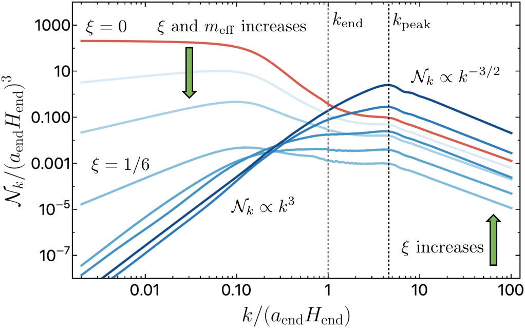
We illustrate the characteristic dependence of the comoving number density spectrum on in Fig. 1. We note that typically peaks at , where is the mode that reenters the horizon at the end of inflation.
The mode , and the short-wavelength (UV) tail of the spectrum, correspond to modes that remain inside the horizon during inflation. For , the spectrum scales as (), independently of the value of . The amplitude of at increases with increasing value of the coupling .
For a large coupling , the effective mass (2) increases, along with the parameter , and the spectrum becomes suppressed in the IR. The same effect occurs in the case of direct DM-inflaton coupling Garcia et al. 2023a; Garcia et al. 2023b. The dominant contribution to gravitational particle production occurs when the standard adiabaticity condition is violated, . When the coupling is very large, , and the transition from quasi-dS to a matter- or radiation-dominated universe causes the effective mass to change rapidly, leading to substantial particle production. Furthermore, when becomes very large (and is imaginary), we find that ().
To determine the present DM relic abundance, one must compute the comoving number density (5) beyond the end of the reheating epoch. We define reheating to occur at time , when the inflaton energy density equals the energy density of the produced radiation, . The reheating temperature is then computed through the corresponding expression Garcia et al. 2021
| (6) |
where represents the effective number of relativistic degrees of freedom at reheating, is the reheating temperature, and is the inflaton perturbative decay rate, with corresponding to an effective Yukawa-like coupling and is the inflaton mass.
Assuming that reheating occurs significantly after the end of inflation, with , and that the total entropy is conserved after the end of reheating, and using Eq. (5), we find that the DM relic density can be expressed as Garcia et al. 2023a
| (7) |
Here, is the rescaled dimensionless comoving momentum, with , is the present Hubble parameter, is the present critical energy density, with Aghanim et al. 2020, and the present comoving scale (IR cutoff) is given by Martin and Ringeval 2010; Liddle and Leach 2003; Ellis et al. 2015; Garcia et al. 2023a. We must ensure that the measured DM relic abundance satisfies the experimental value Aghanim et al. 2020, and it is obtained at some reheating temperature in the range with the BBN temperature of and , which is the theoretical maximum temperature, corresponding to the instantaneous conversion of the total inflaton energy density to radiation at the end of inflation.
Resonant Dark Matter Production.— When the nonminimal coupling is large, with , the mode equation (4) takes the form of a Mathieu equation, which features parametric instabilities. These instabilities give rise to exponential quasi-stochastic excitations of modes , as discussed further in the Supplementary Material. To account for such effects, one must rely on full numerical solutions to the mode equation. Our analysis incorporates parametric resonance effects up to . For larger values, namely , such an extensive excitation corresponds to a dark matter energy density that exceeds one percent of the inflaton energy density. This would lead to the fragmentation of the inflaton condensate and backreaction on the scalar curvature . To account for these effects, one must employ more advanced tools, such as lattice simulations, as explored in Ref. Figueroa et al. 2021; Lebedev et al. 2023. However, the lattice studies lie beyond the scope of this work and we do not consider them here.
Thermal Production of Dark Matter.— Since the transition from a matter-dominated to radiation-dominated universe can be slow, one must also account for the thermal production of DM through the gravitational scattering of Standard Model (SM) particles from the thermal bath Bernal et al. 2018; Mambrini and Olive 2021; Clery et al. 2022a; Clery et al. 2022b; Haque and Maity 2021. In this case, dark matter is generated via freeze-in during the reheating phase. The dark matter density can be inferred by solving the system of coupled differential equations describing the inflaton decay and reheating,
| (8) | ||||
| (9) | ||||
| (10) |
where and are the energy density of the inflaton and radiation, respectively, and is the temperature-dependent thermal production rate. By considering this rate to be subdominant compared to the inflaton decay rate, we have neglected the corresponding term accounting for DM production on the right-hand side of the second equation, only mildly affecting the radiation energy density. The radiation temperature can be estimated by solving the first two equations. The equation for the DM number density can be determined by solving the Boltzmann equation expressed in terms of the comoving number density ,
| (11) |
We find that the total thermal production rate induced by all gravitational scattering processes is given by
| (12) |
and the thermally-produced DM relic abundance is
| (13) |
We note that for couplings and the thermal rate is identical and reduces to the result found in Clery et al. 2022a. When the nonminimal coupling is large, the rate becomes . The detailed calculations are given in the Supplemental Material (SM).
Isocurvature Constraints.— When a light scalar dark matter field (spectator field) is excited during inflation, it inevitably leads to large isocurvature perturbations Chung et al. 2005; Chung and Yoo 2013. The rapid increase in dark matter energy density is primarily driven by the quadratic fluctuations that substantially contribute to the variance Chung et al. 2005; Chung and Yoo 2015; Ling and Long 2021; Redi and Tesi 2022. Our analysis assumes no initial misalignment for the dark matter scalar field at the beginning of inflation, with , (and ) Starobinsky and Yokoyama 1994; Garcia et al. 2023b. Notably, when , the dark matter inhomogeneities do not directly affect the curvature perturbation, and they can be treated as pure isocurvature fluctuations in the comoving gauge Chung and Yoo 2013; Chung et al. 2005. The second-order contribution to the isocurvature power spectrum is given by Liddle and Mazumdar 2000; Chung et al. 2005; Ling and Long 2021
| (14) |
where and denote the DM energy density and its fluctuation, respectively. The current constraints on the isocurature power spectrum provided by are at the 95% C.L. for the pivot scale , where is the curvature power spectrum Akrami et al. 2020. This imposes an upper limit on the isocurvature power spectrum . To understand the isocurvature suppression intuitively, one can compute the variance averaged over the superhorizon modes, with , and regard such long-wavelength contribution as coherent oscillations of the DM field Ema et al. 2018; Tenkanen 2019. Approximating that the field displacement at the end of inflation is given by , with the energy density given by , the isocurvature power spectrum becomes proportional to ; it becomes more suppressed as , and in turn , increases. However, to account for the full spectrum evolution including the transitions, one must evaluate numerically Eq. (14).
For purely gravitational dark matter production, the isocurvature constraints from Planck require that , where is the Hubble scale at the horizon exit. For a minimal coupling (), this constraint becomes Garcia et al. 2023b. Assuming a very light bare dark matter mass, with , we find that the isocurvature limits are always avoided for . This implies that even a very small value of a nonminimal coupling is sufficient to satisfy Planck isocurvature limits, and the conformal coupling case always satisfies the constraint.
Lyman- Forest Constraints.— In contrast to the conventional WIMP scenario, light dark matter particles produced in an out-of-equilibrium state may possess a considerable pressure component, resulting in the suppression of overdensities on galactic scales and subsequently implying a cutoff in the matter power spectrum for scales larger than the free-streaming horizon wavenumber . Lyman- forest measurements constrain such cutoff scale to be around . This can be translated into a lower limit on the mass of a generic warm dark matter (WDM) candidate decoupling from the thermal bath Narayanan et al. 2000; Viel et al. 2005; Viel et al. 2013; Baur et al. 2016; Irsic et al. 2017; Palanque-Delabrouille et al. 2020; Garzilli et al. 2019
For DM produced in an out-of-equilibrium state, one can translate the Lyman- bound into a constraint on the DM mass by matching the corresponding equation of state parameters. This process leads to the following bound Ballesteros et al. 2021; Garcia et al. 2023a
| (15) |
where is the WDM temperature saturating the dark matter abundance 33 3 This quantity only depends on , see Ref. Ballesteros et al. 2021 for details.. is the characteristic energy scale of the produced DM, and the normalized second moment of the dark matter phase space distribution function defined by
| (16) |
For a WDM candidate, this quantity is approximately . We argue that large values of nonminimal coupling allow the scalar dark matter to be very light, and the values of can be constrained by the structure formation limits, as detailed in our parameter space analysis below.
Results and Discussion.— To impose the model constraints and demonstrate the effect of a nonminimal coupling , we consider the T-model inflationary potential Kallosh and Linde 2013
| (17) |
where the potential can be normalized using the approximation Garcia et al. 2021. For a nominal choice of -folds, we obtain , the spectral tilt , and the tensor-to-scalar ratio , which is highly favored by current CMB measurements Akrami et al. 2020; Ellis et al. 2021. The parameter determines the inflaton mass at the potential minimum , with . The Hubble parameter at the horizon exit is given by (with ), and at the end of inflation, .
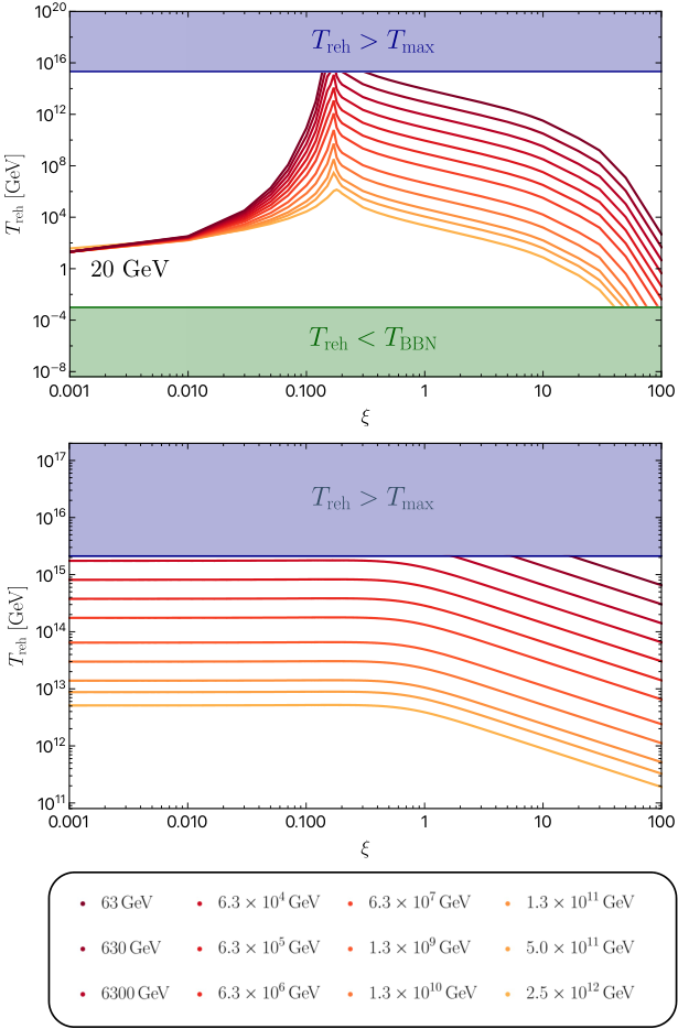
To determine how gravitational particle production depends on the nonminimal coupling and the reheating temperature , we compute the DM relic density using Eq. (7) and impose the observational value Aghanim et al. 2020. Since the relic abundance depends on the reheating temperature, we apply the reheating temperature limits , where the BBN temperature is and . We illustrate in the top panel of Fig. 2 the reheating temperature as a function of for a range of masses varying from to . We find that when , as a universal limit is reached, with . As increases, the reheating temperature peaks in the range of , and the conformal coupling lies in this domain. Intuitively, this result can be better understood from Fig. 1: when the nonminimal coupling is close to the conformal coupling value of , both the long-wavelength (IR) and the short-wavelength (UV) modes become suppressed in the comoving number density spectrum , and the total gravitationally-produced DM abundance is significantly reduced, which necessitates a very high reheating temperature to match the experimental value of . However, as increases to larger values, the short-wavelength (UV) modes become the dominant contribution in the spectrum, and the required reheating temperatures now decrease exponentially. We find that for , the reheating temperature function can be fitted with the expression , where and .
Next, we use the thermal DM relic density expression (13) and display in the bottom panel of Fig. 2. As can be observed, the thermally produced DM requires an extremely large reheating temperature close to . However, when comparing it with the purely gravitational particle production (top panel), we can see that the thermal production remains subdominant throughout the entire parameter space. Lastly, when evaluating cosmological parameters, it is important to adhere to the validity of the low-energy theory. The cutoff of this theory, which in this instance is the reheating temperature, can be approximated as Bezrukov et al. 2011. From our numerical analysis, we find that this constraint is always less stringent than the constraint.
To impose the isocurvature constraints, we numerically compute the isocurvature power spectrum (14) while imposing an experimental upper bound Aghanim et al. 2020. We find that the fully numerical results are in excellent agreement with our given analytical approximations presented above. For minimal coupling, we find that , which agrees with the well-known results that a scalar dark matter field with minimal coupling must be superheavy Chung et al. 2005; Chung and Yoo 2013; Ling and Long 2021; for a conformal coupling , we find that the isocurvature constraints are always satisfied, and in the massless limit we find that .
Finally, we estimate the Lyman- bound (15). We find that the dark matter bound increases as a function of , with when , and it plateaus around , with the bound given by . The details of our derivation can be found in the Supplementary Material sections.
We show our combined parameter space in Fig. 3. In general, the nonminimal coupling is constrained to , with the lower bound resulting from the isocurvature constraint and the upper value from the BBN constraint. We note that we have not studied the superheavy region , which would also have constraints arising from and , and we plan to investigate this in future work. We found that Lyman- constraints give the lower bound . The strongest constraint arises from in the range of .
In this Letter, we have explored a simple and compelling scenario involving a spectator DM scalar field that couples nonminimally to gravity. Our study demonstrates that the presence of nonminimal coupling opens up a broad parameter space, subject to constrains arising from maximum reheating temperature, BBN temperature, isocurvature, Lyman- limits. We look forward to forthcoming experiments such as the Simons Observatory Ade et al. 2019, CMB-S4 Abazajian et al. 2019, and LiteBIRD Hazumi et al. 2019, which could potentially detect B-modes in the CMB, provide more comprehensive scalar power spectrum analysis, and either strengthen isocurvature mode constraints or detect it. Since in this scenario, the DM field contains a blue-tilted isocurvature component, it predicts an enhancement in the power spectrum at small scales, making it amenable for being further constrained by improved structure formation and spectral distortion data Newton et al. 2021; Kogut et al. 2011; Fu et al. 2021. We plan to extend our study and examine the superheavy mass regime and DM self-interaction effects in the upcoming work.
Acknowledgements.
We thank Mustafa Amin, Veronica Guidetti, Oleg Lebedev, Andrew Long, Konstantin Matchev, Michele Redi, and Jong-Hyun Yoon for helpful discussions. MG is supported by the DGAPA-PAPIIT grant IA103123 at UNAM, and the CONAHCYT “Ciencia de Frontera” grant CF-2023-I-17. MP acknowledges support by the Deutsche Forschungsgemeinschaft (DFG, German Research Foundation) under Germany’s Excellence Strategy – EXC 2121 “Quantum Universe” – 390833306. The work of S.V. was supported in part by DOE grant DE-SC0022148.References
- Workman et al. (2022) R. L. Workman et al. (Particle Data Group), “Review of Particle Physics,” PTEP 2022, 083C01 (2022).
- Rubin and Ford (1970) Vera C. Rubin and W. Kent Ford, Jr., “Rotation of the Andromeda Nebula from a Spectroscopic Survey of Emission Regions,” Astrophys. J. 159, 379–403 (1970).
- Aprile et al. (2018) E. Aprile et al. (XENON), “Dark Matter Search Results from a One Ton-Year Exposure of XENON1T,” Phys. Rev. Lett. 121, 111302 (2018), arXiv:1805.12562 [astro-ph.CO] .
- Akerib et al. (2017) D. S. Akerib et al. (LUX), “Results from a search for dark matter in the complete LUX exposure,” Phys. Rev. Lett. 118, 021303 (2017), arXiv:1608.07648 [astro-ph.CO] .
- Meng et al. (2021) Yue Meng et al. (PandaX-4T), “Dark Matter Search Results from the PandaX-4T Commissioning Run,” Phys. Rev. Lett. 127, 261802 (2021), arXiv:2107.13438 [hep-ex] .
- Aalbers et al. (2022) J. Aalbers et al. (LZ), “First Dark Matter Search Results from the LUX-ZEPLIN (LZ) Experiment,” (2022), arXiv:2207.03764 [hep-ex] .
- Arcadi et al. (2018) Giorgio Arcadi, Maíra Dutra, Pradipta Ghosh, Manfred Lindner, Yann Mambrini, Mathias Pierre, Stefano Profumo, and Farinaldo S. Queiroz, “The waning of the WIMP? A review of models, searches, and constraints,” Eur. Phys. J. C 78, 203 (2018), arXiv:1703.07364 [hep-ph] .
- Escudero et al. (2016) Miguel Escudero, Asher Berlin, Dan Hooper, and Meng-Xiang Lin, “Toward (Finally!) Ruling Out Z and Higgs Mediated Dark Matter Models,” JCAP 12, 029 (2016), arXiv:1609.09079 [hep-ph] .
- Mambrini (2021) Y. Mambrini, Particles in the dark Universe, ISBN 978-3-030-78139-2 (Springer, 2021).
- Parker (1968) L. Parker, “Particle creation in expanding universes,” Phys. Rev. Lett. 21, 562–564 (1968).
- Parker (1969) Leonard Parker, “Quantized fields and particle creation in expanding universes. 1.” Phys. Rev. 183, 1057–1068 (1969).
- Ford (1987) L. H. Ford, “Gravitational Particle Creation and Inflation,” Phys. Rev. D 35, 2955 (1987).
- Ema et al. (2018) Yohei Ema, Kazunori Nakayama, and Yong Tang, “Production of Purely Gravitational Dark Matter,” JHEP 09, 135 (2018), arXiv:1804.07471 [hep-ph] .
- Chung et al. (1999) Daniel J. H. Chung, Edward W. Kolb, and Antonio Riotto, “Production of massive particles during reheating,” Phys. Rev. D 60, 063504 (1999), arXiv:hep-ph/9809453 .
- Garcia et al. (2023a) Marcos A. G. Garcia, Mathias Pierre, and Sarunas Verner, “Scalar dark matter production from preheating and structure formation constraints,” Phys. Rev. D 107, 043530 (2023a), arXiv:2206.08940 [hep-ph] .
- Ema et al. (2015) Yohei Ema, Ryusuke Jinno, Kyohei Mukaida, and Kazunori Nakayama, “Gravitational Effects on Inflaton Decay,” JCAP 05, 038 (2015), arXiv:1502.02475 [hep-ph] .
- Ema et al. (2016) Yohei Ema, Ryusuke Jinno, Kyohei Mukaida, and Kazunori Nakayama, “Gravitational particle production in oscillating backgrounds and its cosmological implications,” Phys. Rev. D 94, 063517 (2016), arXiv:1604.08898 [hep-ph] .
- Chung et al. (2005) Daniel J. H. Chung, Edward W. Kolb, Antonio Riotto, and Leonardo Senatore, “Isocurvature constraints on gravitationally produced superheavy dark matter,” Phys. Rev. D 72, 023511 (2005), arXiv:astro-ph/0411468 .
- Chung and Yoo (2013) Daniel J. H. Chung and Hojin Yoo, “Isocurvature Perturbations and Non-Gaussianity of Gravitationally Produced Nonthermal Dark Matter,” Phys. Rev. D 87, 023516 (2013), arXiv:1110.5931 [astro-ph.CO] .
- Chung and Yoo (2015) Daniel J. H. Chung and Hojin Yoo, “Elementary Theorems Regarding Blue Isocurvature Perturbations,” Phys. Rev. D 91, 083530 (2015), arXiv:1501.05618 [astro-ph.CO] .
- Herring et al. (2020) Nathan Herring, Daniel Boyanovsky, and Andrew R. Zentner, “Nonadiabatic cosmological production of ultralight dark matter,” Phys. Rev. D 101, 083516 (2020), arXiv:1912.10859 [gr-qc] .
- Padilla et al. (2019) Luis E. Padilla, J. Alberto Vázquez, Tonatiuh Matos, and Gabriel Germán, “Scalar Field Dark Matter Spectator During Inflation: The Effect of Self-interaction,” JCAP 05, 056 (2019), arXiv:1901.00947 [astro-ph.CO] .
- Ling and Long (2021) Siyang Ling and Andrew J. Long, “Superheavy scalar dark matter from gravitational particle production in -attractor models of inflation,” Phys. Rev. D 103, 103532 (2021), arXiv:2101.11621 [astro-ph.CO] .
- Redi and Tesi (2022) Michele Redi and Andrea Tesi, “Dark photon Dark Matter without Stueckelberg mass,” JHEP 10, 167 (2022), arXiv:2204.14274 [hep-ph] .
- Cosme et al. (2018a) Catarina Cosme, João G. Rosa, and O. Bertolami, “Scalar field dark matter with spontaneous symmetry breaking and the keV line,” Phys. Lett. B 781, 639–644 (2018a), arXiv:1709.09674 [hep-ph] .
- Cosme et al. (2018b) Catarina Cosme, João G. Rosa, and O. Bertolami, “Scale-invariant scalar field dark matter through the Higgs portal,” JHEP 05, 129 (2018b), arXiv:1802.09434 [hep-ph] .
- Alonso-Álvarez and Jaeckel (2018) Gonzalo Alonso-Álvarez and Joerg Jaeckel, “Lightish but clumpy: scalar dark matter from inflationary fluctuations,” JCAP 10, 022 (2018), arXiv:1807.09785 [hep-ph] .
- Fairbairn et al. (2019) Malcolm Fairbairn, Kimmo Kainulainen, Tommi Markkanen, and Sami Nurmi, “Despicable Dark Relics: generated by gravity with unconstrained masses,” JCAP 04, 005 (2019), arXiv:1808.08236 [astro-ph.CO] .
- Alonso-Álvarez et al. (2020) Gonzalo Alonso-Álvarez, Thomas Hugle, and Joerg Jaeckel, “Misalignment \& Co.: (Pseudo-)scalar and vector dark matter with curvature couplings,” JCAP 02, 014 (2020), arXiv:1905.09836 [hep-ph] .
- Kolb et al. (2023) Edward W. Kolb, Andrew J. Long, Evan McDonough, and Guillaume Payeur, “Completely dark matter from rapid-turn multifield inflation,” JHEP 02, 181 (2023), arXiv:2211.14323 [hep-th] .
- Misner et al. (1973) Charles W. Misner, K. S. Thorne, and J. A. Wheeler, Gravitation (W. H. Freeman, San Francisco, 1973).
- Garcia et al. (2023b) Marcos A. G. Garcia, Mathias Pierre, and Sarunas Verner, “Isocurvature Constraints on Scalar Dark Matter Production from the Inflaton,” (2023b), arXiv:2303.07359 [hep-ph] .
- Akrami et al. (2020) Y. Akrami et al. (Planck), “Planck 2018 results. X. Constraints on inflation,” Astron. Astrophys. 641, A10 (2020), arXiv:1807.06211 [astro-ph.CO] .
- Kofman et al. (1997) Lev Kofman, Andrei D. Linde, and Alexei A. Starobinsky, “Towards the theory of reheating after inflation,” Phys. Rev. D 56, 3258–3295 (1997), arXiv:hep-ph/9704452 .
- Garcia et al. (2022) Marcos A. G. Garcia, Kunio Kaneta, Yann Mambrini, Keith A. Olive, and Sarunas Verner, “Freeze-in from preheating,” JCAP 03, 016 (2022), arXiv:2109.13280 [hep-ph] .
- Starobinsky and Yokoyama (1994) Alexei A. Starobinsky and Junichi Yokoyama, “Equilibrium state of a selfinteracting scalar field in the De Sitter background,” Phys. Rev. D 50, 6357–6368 (1994), arXiv:astro-ph/9407016 .
- Kaneta et al. (2022) Kunio Kaneta, Sung Mook Lee, and Kin-ya Oda, “Boltzmann or Bogoliubov? Approaches compared in gravitational particle production,” JCAP 09, 018 (2022), arXiv:2206.10929 [astro-ph.CO] .
- Garcia et al. (2021) Marcos A. G. Garcia, Kunio Kaneta, Yann Mambrini, and Keith A. Olive, “Inflaton Oscillations and Post-Inflationary Reheating,” JCAP 04, 012 (2021), arXiv:2012.10756 [hep-ph] .
- Aghanim et al. (2020) N. Aghanim et al. (Planck), “Planck 2018 results. VI. Cosmological parameters,” Astron. Astrophys. 641, A6 (2020), [Erratum: Astron.Astrophys. 652, C4 (2021)], arXiv:1807.06209 [astro-ph.CO] .
- Martin and Ringeval (2010) Jerome Martin and Christophe Ringeval, “First CMB Constraints on the Inflationary Reheating Temperature,” Phys. Rev. D 82, 023511 (2010), arXiv:1004.5525 [astro-ph.CO] .
- Liddle and Leach (2003) Andrew R Liddle and Samuel M Leach, “How long before the end of inflation were observable perturbations produced?” Phys. Rev. D 68, 103503 (2003), arXiv:astro-ph/0305263 .
- Ellis et al. (2015) John Ellis, Marcos A. G. Garcia, Dimitri V. Nanopoulos, and Keith A. Olive, “Calculations of Inflaton Decays and Reheating: with Applications to No-Scale Inflation Models,” JCAP 07, 050 (2015), arXiv:1505.06986 [hep-ph] .
- Figueroa et al. (2021) Daniel G. Figueroa, Adrien Florio, Toby Opferkuch, and Ben A. Stefanek, “Dynamics of Non-minimally Coupled Scalar Fields in the Jordan Frame,” (2021), arXiv:2112.08388 [astro-ph.CO] .
- Lebedev et al. (2023) Oleg Lebedev, Timofey Solomko, and Jong-Hyun Yoon, “Dark matter production via a non-minimal coupling to gravity,” JCAP 02, 035 (2023), arXiv:2211.11773 [hep-ph] .
- Bernal et al. (2018) Nicolás Bernal, Maíra Dutra, Yann Mambrini, Keith Olive, Marco Peloso, and Mathias Pierre, “Spin-2 Portal Dark Matter,” Phys. Rev. D 97, 115020 (2018), arXiv:1803.01866 [hep-ph] .
- Mambrini and Olive (2021) Yann Mambrini and Keith A. Olive, “Gravitational Production of Dark Matter during Reheating,” Phys. Rev. D 103, 115009 (2021), arXiv:2102.06214 [hep-ph] .
- Clery et al. (2022a) Simon Clery, Yann Mambrini, Keith A. Olive, and Sarunas Verner, “Gravitational portals in the early Universe,” Phys. Rev. D 105, 075005 (2022a), arXiv:2112.15214 [hep-ph] .
- Clery et al. (2022b) Simon Clery, Yann Mambrini, Keith A. Olive, Andrey Shkerin, and Sarunas Verner, “Gravitational portals with nonminimal couplings,” Phys. Rev. D 105, 095042 (2022b), arXiv:2203.02004 [hep-ph] .
- Haque and Maity (2021) Md Riajul Haque and Debaprasad Maity, “Gravitational dark matter: free streaming and phase space distribution,” (2021), arXiv:2112.14668 [hep-ph] .
- Liddle and Mazumdar (2000) Andrew R Liddle and Anupam Mazumdar, “Perturbation amplitude in isocurvature inflation scenarios,” Phys. Rev. D 61, 123507 (2000), arXiv:astro-ph/9912349 .
- Tenkanen (2019) Tommi Tenkanen, “Dark matter from scalar field fluctuations,” Phys. Rev. Lett. 123, 061302 (2019), arXiv:1905.01214 [astro-ph.CO] .
- Narayanan et al. (2000) Vijay K. Narayanan, David N. Spergel, Romeel Dave, and Chung-Pei Ma, “Constraints on the mass of warm dark matter particles and the shape of the linear power spectrum from the Ly forest,” Astrophys. J. Lett. 543, L103–L106 (2000), arXiv:astro-ph/0005095 .
- Viel et al. (2005) Matteo Viel, Julien Lesgourgues, Martin G. Haehnelt, Sabino Matarrese, and Antonio Riotto, “Constraining warm dark matter candidates including sterile neutrinos and light gravitinos with WMAP and the Lyman-alpha forest,” Phys. Rev. D 71, 063534 (2005), arXiv:astro-ph/0501562 .
- Viel et al. (2013) Matteo Viel, George D. Becker, James S. Bolton, and Martin G. Haehnelt, “Warm dark matter as a solution to the small scale crisis: New constraints from high redshift Lyman- forest data,” Phys. Rev. D 88, 043502 (2013), arXiv:1306.2314 [astro-ph.CO] .
- Baur et al. (2016) Julien Baur, Nathalie Palanque-Delabrouille, Christophe Yèche, Christophe Magneville, and Matteo Viel, “Lyman-alpha Forests cool Warm Dark Matter,” JCAP 08, 012 (2016), arXiv:1512.01981 [astro-ph.CO] .
- Irsic et al. (2017) Vid Irsic et al., “New Constraints on the free-streaming of warm dark matter from intermediate and small scale Lyman- forest data,” Phys. Rev. D 96, 023522 (2017), arXiv:1702.01764 [astro-ph.CO] .
- Palanque-Delabrouille et al. (2020) Nathalie Palanque-Delabrouille, Christophe Yèche, Nils Schöneberg, Julien Lesgourgues, Michael Walther, Solène Chabanier, and Eric Armengaud, “Hints, neutrino bounds and WDM constraints from SDSS DR14 Lyman- and Planck full-survey data,” JCAP 04, 038 (2020), arXiv:1911.09073 [astro-ph.CO] .
- Garzilli et al. (2019) A. Garzilli, O. Ruchayskiy, A. Magalich, and A. Boyarsky, “How warm is too warm? Towards robust Lyman- forest bounds on warm dark matter,” (2019), arXiv:1912.09397 [astro-ph.CO] .
- Ballesteros et al. (2021) Guillermo Ballesteros, Marcos A. G. Garcia, and Mathias Pierre, “How warm are non-thermal relics? Lyman- bounds on out-of-equilibrium dark matter,” JCAP 03, 101 (2021), arXiv:2011.13458 [hep-ph] .
- Kallosh and Linde (2013) Renata Kallosh and Andrei Linde, “Non-minimal Inflationary Attractors,” JCAP 10, 033 (2013), arXiv:1307.7938 [hep-th] .
- Ellis et al. (2021) John Ellis, Marcos A. G. Garcia, Dimitri V. Nanopoulos, Keith A. Olive, and Sarunas Verner, “BICEP/Keck Constraints on Attractor Models of Inflation and Reheating,” (2021), arXiv:2112.04466 [hep-ph] .
- Bezrukov et al. (2011) F. Bezrukov, A. Magnin, M. Shaposhnikov, and S. Sibiryakov, “Higgs inflation: consistency and generalisations,” JHEP 01, 016 (2011), arXiv:1008.5157 [hep-ph] .
- Ade et al. (2019) Peter Ade et al. (Simons Observatory), “The Simons Observatory: Science goals and forecasts,” JCAP 02, 056 (2019), arXiv:1808.07445 [astro-ph.CO] .
- Abazajian et al. (2019) Kevork Abazajian et al., “CMB-S4 Science Case, Reference Design, and Project Plan,” (2019), arXiv:1907.04473 [astro-ph.IM] .
- Hazumi et al. (2019) M. Hazumi et al., “LiteBIRD: A Satellite for the Studies of B-Mode Polarization and Inflation from Cosmic Background Radiation Detection,” J. Low Temp. Phys. 194, 443–452 (2019).
- Newton et al. (2021) Oliver Newton, Matteo Leo, Marius Cautun, Adrian Jenkins, Carlos S. Frenk, Mark R. Lovell, John C. Helly, Andrew J. Benson, and Shaun Cole, “Constraints on the properties of warm dark matter using the satellite galaxies of the Milky Way,” JCAP 08, 062 (2021), arXiv:2011.08865 [astro-ph.CO] .
- Kogut et al. (2011) A. Kogut et al., “The Primordial Inflation Explorer (PIXIE): A Nulling Polarimeter for Cosmic Microwave Background Observations,” JCAP 07, 025 (2011), arXiv:1105.2044 [astro-ph.CO] .
- Fu et al. (2021) Hao Fu, Matteo Lucca, Silvia Galli, Elia S. Battistelli, Deanna C. Hooper, Julien Lesgourgues, and Nils Schöneberg, “Unlocking the synergy between CMB spectral distortions and anisotropies,” JCAP 12, 050 (2021), arXiv:2006.12886 [astro-ph.CO] .
- Ellis et al. (2013) John Ellis, Dimitri V. Nanopoulos, and Keith A. Olive, “Starobinsky-like Inflationary Models as Avatars of No-Scale Supergravity,” JCAP 10, 009 (2013), arXiv:1307.3537 [hep-th] .
- Fixsen (2009) D. J. Fixsen, “The Temperature of the Cosmic Microwave Background,” Astrophys. J. 707, 916–920 (2009), arXiv:0911.1955 [astro-ph.CO] .
- Giudice et al. (2001) Gian Francesco Giudice, Edward W. Kolb, and Antonio Riotto, “Largest temperature of the radiation era and its cosmological implications,” Phys. Rev. D 64, 023508 (2001), arXiv:hep-ph/0005123 .
- Holstein (2006) Barry R. Holstein, “Graviton Physics,” Am. J. Phys. 74, 1002–1011 (2006), arXiv:gr-qc/0607045 .
- Birrell and Davies (1984) N. D. Birrell and P. C. W. Davies, Quantum Fields in Curved Space, Cambridge Monographs on Mathematical Physics (Cambridge Univ. Press, Cambridge, UK, 1984).
- Giudice et al. (1999) Gian F. Giudice, Riccardo Rattazzi, and James D. Wells, “Quantum gravity and extra dimensions at high-energy colliders,” Nucl. Phys. B 544, 3–38 (1999), arXiv:hep-ph/9811291 .
- Anastasopoulos et al. (2020) Pascal Anastasopoulos, Kunio Kaneta, Yann Mambrini, and Mathias Pierre, “Energy-momentum portal to dark matter and emergent gravity,” Phys. Rev. D 102, 055019 (2020), arXiv:2007.06534 [hep-ph] .
- Brax et al. (2021a) Philippe Brax, Kunio Kaneta, Yann Mambrini, and Mathias Pierre, “Disformal dark matter,” Phys. Rev. D 103, 015028 (2021a), arXiv:2011.11647 [hep-ph] .
- Brax et al. (2021b) Philippe Brax, Kunio Kaneta, Yann Mambrini, and Mathias Pierre, “Metastable Conformal Dark Matter,” Phys. Rev. D 103, 115016 (2021b), arXiv:2103.02615 [hep-ph] .
- Vilenkin (1983) Alexander Vilenkin, “Quantum Fluctuations in the New Inflationary Universe,” Nucl. Phys. B 226, 527–546 (1983).
- Mukhanov et al. (1992) Viatcheslav F. Mukhanov, H. A. Feldman, and Robert H. Brandenberger, “Theory of cosmological perturbations. Part 1. Classical perturbations. Part 2. Quantum theory of perturbations. Part 3. Extensions,” Phys. Rept. 215, 203–333 (1992).
- Enqvist et al. (1988) K. Enqvist, K. W. Ng, and Keith A. Olive, “Scalar Field Fluctuations in the Early Universe,” Nucl. Phys. B 303, 713 (1988).
Supplementary Material for A New Window into Gravitationally Produced Scalar Dark Matter
Marcos A. G. Garcia, Mathias Pierre, and Sarunas Verner
This Supplementary Material (SM) is organized as follows: In Sec. I, we discuss the dynamics of slow-roll inflation and the reheating mechanism. Subsequently, in Sec. II, we demonstrate the computation of the phase space distributions (PSDs) for the T-model of inflation and calculate the purely thermal production of scalar dark matter. In Sec. III, we present the analytical approximations of the isocurvature constraints. Lastly, in Sec. IV, we discuss the full computation of the Lyman- bound.
I Inflationary Dynamics and Reheating
I.1 Slow-roll inflation
In this section, we review the dynamics of the inflaton field, , using the slow-roll approximation. We consider the following action:
| (S1) |
where the inflaton field is minimally coupled to gravity. Varying this action with respect to leads the Klein-Gordon equation of motion
| (S2) |
where the prime denotes a derivative with respect to the inflaton field, . The Hubble rate is given by
| (S3) |
where is the scale factor. In our analysis, we employ the conventional single-field slow-roll inflationary parameters:
| (S4) |
By using the slow-roll approximation, we find that the number of -folds can be expressed as
| (S5) |
where the star denotes quantities at the horizon exit of , the pivot scale used in the Planck analysis. The end of inflation occurs when , which can be equivalently defined as .
The primary CMB observables, specifically the scalar tilt, , the tensor-to-scalar ratio, , and the amplitude of the curvature power spectrum, , can be expressed in terms of the slow-roll parameters as follows:
| (S6) | ||||
| (S7) | ||||
| (S8) |
where and Aghanim et al. 2020. In our numerical analysis, we consider the T-model of inflation, given by Eq. (17). For this model, using the large limit, one can find the following cosmological observables Ellis et al. 2013
| (S9) |
For a nominal choice -folds, we find that the normalization constant is given by , the spectral tilt , and the tensor-to-scalar ratio . In this subsection, we have presented analytical approximations, and in the next subsection, we describe the full numerical procedure for the inflationary evolution and reheating.
I.2 Reheating
In a more complete analysis, it is necessary to account for the duration of reheating, in order to accurately relate the number of -folds of observable inflation with the Planck pivot scale. We thus compute the total number of -folds, assuming no additional entropy production between the end of reheating and the time when the horizon scale reenters the horizon Martin and Ringeval 2010; Liddle and Leach 2003:
| (S10) |
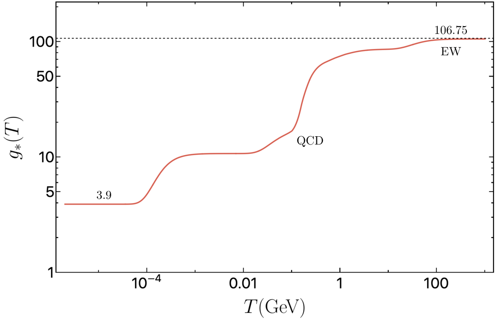
The present Hubble rate is given by Aghanim et al. 2020 and the present photon temperature is Fixsen 2009. Here, and are the energy density at the end of inflation and at the beginning of the radiation domination era when , respectively, is the present day scale factor, and represents the effective number of relativistic degrees of freedom in the Standard Model at time of reheating, typically taken to be for the reheating temperatures higher than . We show the SM relativistic degrees of freedom as a function of the temperature in Fig. S1. We note, that in our full numerical analysis we considered the equation of motion parameter averaged over the -folds during reheating, given by
| (S11) |
where and are the total number of -folds at the end of inflation and at the beginning of full radiation domination era, respectively.
The background dynamics are determined by the following system of coupled Friedmann-Boltzmann equations:
| (S12) | ||||
| (S13) | ||||
| (S14) | ||||
| (S15) |
where is the energy density of the inflaton. Here is the inflaton decay rate defined by
| (S16) |
where is a Yukawa-like coupling. For T-models of inflation (17), we find that the inflaton mass is given by , where . The universe undergoes reheating after the end of inflation, transitioning from a matter-dominated universe to a radiation-dominated universe. As the inflaton starts to decay, the thermal plasma dilutes until a maximum temperature of is reached Giudice et al. 2001. Subsequently, the temperature falls as , and the reheating temperature can be approximated as
| (S17) |
For the T-model of inflation (17), can be determined from the following simplified expression of the general expression (S10) Ellis et al. 2021,
| (S18) |
Numerically, we find that inflation ends when and . We demonstrate the reheating process in Fig. S2 for the T-model of inflation and plot the evolution of energy densities during reheating with a nominal choice of the Yukawa coupling .
II Computing the Scalar Particle Production and the PSDs
II.1 Perturbative gravitational production from the inflaton
Since for gravitational production, DM annihilation, and thermalization can be safely neglected, the only relevant process for the determination of the PSD corresponds to the linear growth of the momentum modes. At the quantum field level, these modes are defined as in Eq. (3), and satisfy the equation of motion (4). To numerically solve for each mode during and after inflation, we use the attractor behavior of the background inflaton dynamics. We begin tracking the modes starting deep inside the horizon (in practice 5 -folds prior to horizon crossing) with Bunch-Davies initial conditions, initial conditions for on the attractor, and unit scale factor at horizon crossing, . This guarantees high precision in the numerical integration. The dark matter PSD can then be evaluated as the particle occupation number
| (S19) |
Here, corresponds to an arbitrarily defined comoving momentum. We find it convenient to refer this comoving momentum to the end of inflation, and introduce its dimensionless form,
| (S20) |
where denotes the physical momentum, and is a characteristic energy scale. In this notation, the comoving DM number density is calculated as
| (S21) |
Fig. S3 shows the numerically determined PSD for 3 different values of the nonminimal coupling . For , the distribution is red-tilted, and has a large amplitude in the IR for . This is the manifestation of the tachyonic de Sitter instability (see “Framework” in the main text). During inflation, modes with have imaginary frequencies, which is translated into their rapid growth. In particular, modes that leave the horizon the earliest grow the most, leading to in the IR Herring et al. 2020; Ling and Long 2021; Kaneta et al. 2022; Garcia et al. 2023a. As Fig. 1 also shows, a larger increases the effective mass of , dampening the growth of the DM modes during inflation, leading to a blue tilt for .
The IR endpoint of the PSD corresponds in principle to the mode that left the horizon at the beginning of inflation. This mode must satisfy , where denotes the re-scaled present horizon scale. Following the standard computation that leads to (S10), this scale may be written as Martin and Ringeval 2010; Liddle and Leach 2003; Ellis et al. 2015
| (S22) |
where Ellis et al. 2021
| (S23) |
From Figs. 1 and S3, we note that for , corresponding to always sub-horizon modes, all PSDs for light DM scale similarly with , although with -dependent amplitudes. The modes are always particle-like, and their contribution to the PSD can be accurately estimated by integration of the Boltzmann equation for the process via graviton exchange during reheating. The dark matter produced from the decay of the inflaton quanta of the oscillating coherent condensate follows the equation
| (S24) |
in the case of a quadratic minimum of , , and Garcia et al. 2023a. The transition amplitude from the condensate to, whose definition can be found in Ref. Garcia et al. 2023a, leads to
| (S25) |
Eq. (S24) can be integrated approximately during reheating accounting for the conversion of into radiation. Denoting as the Heaviside step function, this solution is given by
| (S26) | ||||
| (S27) |
where , for . The exponential tail is a phenomenological fit to (S26) beyond the end of reheating. Due to the decay of the inflaton, during radiation domination, where must be numerically determined following the non-instantaneous transition from to . Fig. S4 shows a comparison between the numerically evaluated PSD and the analytical approximation (S27) for modes excited between the end of inflation and the end of reheating.
Having determined the PSD, the dark matter relic abundance is evaluated by integration of Eq. (7).
II.2 Resonant gravitational production from the inflaton
For large values of , the scalar dark matter candidate is strongly coupled to the oscillating background, whose curvature can be expressed in terms of the inflaton field as
| (S28) |
assuming that the DM energy density is subdominant. After the end of inflation, the background inflaton field can be approximated by
| (S29) |
which can be used to express the Ricci scalar as
| (S30) |
Here we neglected the terms suppressed by powers of that decrease with time. The equation of motion for the rescaled field takes the form of the Mathieu equation
| (S31) |
where , and
| (S32) |
in agreement with Ref. Lebedev et al. 2023. The Mathieu equation contains parametric instabilities. Solutions to this equation may undergo parametric resonances for large values of , i.e., . Such resonances can be seen in the left panel of Fig. S5, where numerical evaluation of the PSD is depicted for chosen values of . For these values of , the UV tail of the distribution consistently matches the perturbative prediction from Eq. (S27), but substantial non-perturbative growth for is apparent for .
Since the coefficients present in the Mathieu equation (S32) have a strong scale factor dependence, the exponential amplification of mode functions typically shuts off rather swiftly after reheating begins, approximatley at , equivalent to inflaton oscillations. However, for exceedingly large values of , backreaction on the inflaton could induce fragmentation of the condensate. Additionally, the background value of the Ricci scalar would depart from the estimate of Eq. (S30) as the dark matter energy density contribution would need to be taken into account. In both cases, our approach, which treats the dark matter as a spectator field, would break down, and one would need to simulate the coupled system of inflaton and dark matter fields on the lattice, which lies beyond the scope of our work and is explored in Ref. Lebedev et al. 2023.
We evaluate the value of where such effects are expected to be significant by noticing that the bulk of the DM energy density is concentrated in modes with , corresponding to modes substantially excited near the end of inflation. This value can therefore be estimated by requiring the dark matter energy density not to exceed of the inflaton energy density at the end of inflation. This corresponds to for and for , as illustrated in the right panel of Fig. S5, in agreement with Ref. Lebedev et al. 2023.
II.3 Gravitational production from the Standard Model plasma
In this section we consider the production of nonminimally coupled scalar dark matter from scatterings between SM particles mediated by gravitational interactions. This contribution to the dark matter abundance can be estimated by solving the Boltzmann equation for the dark matter number density
| (S33) |
where is the thermal production rate that we derive in the following.
Interaction terms. First, we expand the space-time metric around flat space , where represents the canonically-normalized (graviton) metric perturbation Holstein 2006 and the Minkowski metric. The relevant gravitational interactions are described by the following Lagrangian:
| (S34) |
Here and denote the stress-energy tensor of the Standard Model and the dark matter field, respectively. In general, the stress-energy tensor expression depends on the spin of the field, . Assuming that all gravitational scattering processes take place at very high temperatures and neglecting masses of the SM particles, we can express the SM stress-energy tensor in the following form:
| (S35) |
where each component can be written explicitly as
| (S36) | |||||
| (S37) | |||||
| (S38) |
where represents a generic SM fermion, a SM gauge field with corresponding field strength tensor and is the SM Higgs doublet with being the corresponding covariant derivative. We used the symbol . The sums are performed over all SM fields. Non-abelian indices are omitted for clarity. Terms giving rise to scattering processes involving more than two initial states were discarded.
With our conventions, we define the dark matter stress-energy tensor by Birrell and Davies 1984, which can be expressed as44 4 This expression agrees with Ref. Lebedev et al. 2023.
| (S39) |
with and being the covariant derivative in curved space-time. Around the flat Minkowski limit, this expression reduces to
| (S40) |
Scattering amplitudes. The gravitational scattering amplitudes of the dark matter production process can be parametrized by
| (S41) |
where represents the spin of the initial Standard Model states involved in the scattering process. and denote respectively the incoming and outgoing momenta. In this case, denotes the propagator for the canonically-normalized graviton carrying momentum Giudice et al. 1999
| (S42) |
The partial amplitude can be expressed as
| (S43) |
The SM partial amplitudes, , are given by
| (S44) | |||||
| (S45) | |||||
| (S46) | |||||
The corresponding full amplitudes including symmetry factors accounting for initial and final states are
| (S47) | |||
| (S48) | |||
| (S49) |
Production rate. Next, we calculate the production rate for scalar dark matter, , in the presence of nonminimal coupling . This rate can be calculated using the following expression Anastasopoulos et al. 2020; Brax et al. 2021a; Brax et al. 2021b
| (S50) |
with is the Fermi-Dirac or Bose-Einstein () distribution. Here the factor of two accounts for two dark matter particles produced per scattering, denotes the number of each SM species of spin : for 1 complex Higgs doublet, for 8 gluons and 4 electroweak bosons, and for 6 (anti)quarks with 3 colors, 3 (anti)charged leptons and 3 neutrinos. The infinitesimal solid angle is given by
| (S51) |
with and being the angle formed by momenta and , respectively. In the massless limit, one can express the amplitude squared in terms of Mandelstam variables, and , which can be related to the angles and by
| (S52) | ||||
| (S53) |
Substitution and intrgration of (S50) yields the following rate
| (S54) |
Dark matter production. From the rate of Eq. (S54), we can solve the Boltzmann equation (S33) and deduce the contribution to the dark matter abundance produced from the thermal bath
| (S55) |
For the parameter space of interest this contribution is always subdominant compared to gravitational production.
III Isocurvature Constraints
In this section, we provide a detailed analysis of the numerical evaluation of the isocurvature power spectrum. Furthermore, we present a comprehensive analytical derivation based on the approach outlined in Ref. Garcia et al. 2023b.
III.1 Numerical evaluation of the isocurvature constraints.
The isocurvature power spectrum can be evaluated by using the following expression Liddle and Mazumdar 2000; Chung et al. 2005; Ling and Long 2021; Garcia et al. 2023b:
| (S56) |
where the integrand is given by
| (S57) |
For light effective dark matter masses, , the integral of features IR () and colinear () divergences. They are regularized with a lower momentum (IR) cutoff taken as the mode that left the horizon at the beginning of inflation. In principle, the power spectrum must be evaluated after the dark matter decoupling time, which in this case corresponds to the end of reheating. Nevertheless, the argument of (S56) rapidly converges during reheating, and a few () -folds are sufficient to obtain a reasonable approximation for the value of . The integral (S56) is convergent in the UV. Further details can be found in Ref. Garcia et al. 2023b.
Fig. S6 shows the numerically evaluated isocurvature power spectrum for different values of the nonminimal coupling for a light DM scalar with . For this DM mass, the isocurvature constraint at the Planck pivot scale (right vertical dashed line) is averted for .
III.2 Analytical estimate of the isocurvature constraints.
We model the dynamics of the universe during inflation as a de Sitter phase, which is described by a constant accelerated expansion of the universe, with and a constant Hubble rate. We assume that this phase begins at an initial time and concludes at . To determine the isocurvature power spectrum, we solve the mode equation for , expressed as a function of cosmic time and given by
| (S58) |
where is the bare mass of the scalar field, which is assumed to be constant. Assuming Bunch-Davies initial condition and a pure de Sitter phase, the solution to the previous equation can be expressed as
| (S59) |
where is the Hankel function of the first kind, and
| (S60) |
In the large wavelength limit , this solution reduces to
| (S61) |
Neglecting the time derivative of the mode function and using the expression for the DM energy density valid at later times, , we can express Eq. (S56) as:
| (S62) |
where the dark matter field variance is
| (S63) |
with
| (S64) |
Using the description above, we introduce a long-wavelength (IR) and short-wavelength (UV) cutoffs that regularize the power spectrum Vilenkin 1983, given by and . The total duration of de Sitter era is given by , where denotes the duration of inflation in -folds between the CMB pivot scale crossing and the end of inflation. We discuss three distinct regimes in detail:
Massless limit . If the DM mass can be neglected compared to the Hubble scale during the de Sitter phase, then , and the mode function can be expressed as
| (S65) |
and the power spectrum is given by
| (S66) |
and it leads to a scale-invariant power spectrum when and , when . If we combine expression (S65) with (S19), we find the the phase space distribution for long-wavelength (IR) modes scales as , which reduces to for . For , at the end of inflation and the quasi-de Sitter phase, the variance can be approximated as
| (S67) |
Evaluated at the CMB pivot scale, the isocurvature power spectrum (S62) is
| (S68) |
which scales as for .
Limit . In this case , with and the mode function takes the following form Mukhanov et al. 1992; Liddle and Mazumdar 2000:
| (S69) |
which leads to a slightly blue-tilted power spectrum
| (S70) |
In this limit, the PSD scales as . At the end of the quasi-de Sitter phase, the variance becomes
| (S71) |
When the quantity and and , the variance no longer depend on the long-wavelength (IR) modes. In this limit, one can approximate the power spectrum as
| (S72) |
where
| (S73) |
and . This expression implies that the isocurvature power spectrum decays exponentially. We note that the function is insensitive to when . Therefore, the only non-negligible infrared sensitivity in Eq. (S72) arises from the scaling function for a large or equivalently in terms of the infrared cutoff.
Limit . In this limit, where and . The mode function becomes
| (S74) |
where in the previous expression, and
| (S75) |
Here is given by
| (S76) |
with and . Since the first term in the squared brackets is an oscillatory term, with the oscillation frequency , it can be ignored. Thus, in the limit , we obtain
| (S77) |
This approximation works remarkably well even when . The absolute value of the mode function can be approximated as
| (S78) |
and the power spectrum becomes
| (S79) |
In the expression above, is the number of -folds when the mode crosses the horizon . The spectrum is convergent in the IR but exponentially decreases with the total number of -folds after horizon crossing , and afterward it scales as non-relativistic matter. In this case, the field variance at the end of quasi-de Sitter phase becomes Enqvist et al. 1988
| (S80) |
where we considered . In this limit, it becomes evident that the isocurvature power spectrum is exponentially suppressed:
| (S81) |
and for a nominal choice of , we find , a value substantially lower than both present and future constraints on isocurvature perturbations.
Estimate of the constraints. Using Eq. (S81), one finds that the isocurvature constraint is never violated when . In the massless limit with , as shown by Eq. (S68), the isocurvature power spectrum is extremely large, given by for , and the experimental constraint is always violated.
In the regime , we can use the approximate expression (S72) to compute the analytical limits for the choice of parameter and -folds. When , the limit becomes
| (S82) |
and in the massless limit, this bound becomes
| (S83) |
which does not depend on the Hubble rate at the horizon exit, . Importantly, this analytical approximation agrees remarkably well with the full numerical computation.
IV Lyman- Constraints
In the standard CDM model, dark matter is assumed to be a pressureless cold fluid. However, generic broad, non-thermal dark matter distributions, as obtained in the gravitational production scenario, could deviate from this CDM picture. Such a deviation is constrained by the Lyman- forest measurements of the matter power spectrum. In this section, we show the detailed derivation of such constraints for our nonminimally coupled dark matter model.
Non-cold dark matter. For a generic dark matter candidate, the full space-time dependent distribution can be expanded in terms of a background quantity and a small fluctuation as
| (S84) |
where is the momentum of DM particles located at the space coordinate . The Fourier transform of the perturbed distribution can be expanded in terms of Legendre polynomials as
| (S85) |
where is the Fourier space wavenumber with and , where is the rescaled dimensionless dark matter momentum. The Legendre coefficients satisfy a system of Boltzmann equations involving metric perturbations as given in Ref. Ballesteros et al. 2021. As argued in the same reference, terms with are typically suppressed for sufficiently cold relics, i.e. for an EOS parameter defined as the ratio of the pressure to the energy density perturbation for the DM species. In this case, this system of equations reduces to a coupled system of continuity and Euler equations for the dark matter relative energy-density perturbation and the velocity perturbation. During matter domination, the equation for the dark matter overdensity becomes Ballesteros et al. 2021
| (S86) |
where is the conformal Hubble rate and is the (time-dependent) free-streaming wave number given by
| (S87) |
This free-streaming wave number, uniquely determined by the EOS , corresponds to a cutoff in the matter power spectrum as compared to the standard CDM cosmology (with ) at the free-streaming horizon scale , solely determined by :
| (S88) |
The equation of state can be related to the normalized second moment of the DM background distribution
| (S89) |
with
| (S90) |
Lyman- constraints. Lyman- forest measurements provide a bound on the cutoff scale to . This can be translated into a lower limit on the DM equation of state for a typical warm dark matter candidate
| (S91) |
This corresponds to a constraint on the mass of a generic warm dark matter (WDM) candidate priorily in thermal equilibrium with the SM bath that decoupled while still relativistic Narayanan et al. 2000; Viel et al. 2005; Viel et al. 2013; Baur et al. 2016; Irsic et al. 2017; Palanque-Delabrouille et al. 2020; Garzilli et al. 2019. From Eq. (S90) and Eq. (S91) one deduces the following bound for a dark matter candidate with a given distribution
| (S92) |
where is the WDM temperature saturating the dark matter abundance. From Eq. (S92), we get the following constraint for our setup
| (S93) |
where the terms inside the squared brackets depend on the bare dark matter mass and nonminimal coupling. The dependence of on these parameters comes from the requirement for the dark matter to saturate the relic abundance.
Constraints for . In this case, as for the large direct DM-inflaton coupling regime of Garcia et al. 2023a, the second moment is UV dominated and depends on the reheating temperature through
| (S94) |
Interestingly, this scaling allows to cancel out the dependence of Eq. (S93) which asymptotes to a -independent value for at
| (S95) |
Parametric resonances induce slight deviations from this relation based on the perturbative (Boltzmann) result. It is important to note that for , the DM relic density scales as . One can therefore rescale the reheating temperature by a factor , such that the correct relic abundance is achieved. Importantly, this factor accounts for deviations from the perturbative (Boltzmann) prediction. Similarly, one can define a coefficient . The constraints of Eq. (S93) can thus be rescaled by an overall factor of . Numerically, we find that such a factor does not significantly depart from unity for the range of interest . Therefore, for simplicity, we can approximate the Lyman- bound by Eq. (S95) for large values of up to the backreaction regime .
Constraints for . In this case, the PSD and corresponding second moment become sensitive to the IR part. In that case, Eq. (S93) has to be evaluated numerically to account for the and simultaneous dependence on and . As the nonminimal coupling decreases, the Lyman- bound approaches the limit for the pure gravitational production bound for a minimally coupled (e.g. ) dark matter candidate Garcia et al. 2023a
| (S96) |
The full numerical results are depicted in Fig. 3, that are found from a numerical evaluation of Eq. (S93).