NCHO: Unsupervised Learning for
Neural 3D Composition of Humans and Objects

Taeksoo Kim Shunsuke Saito Hanbyul Joo Affiliation: Seoul National University Affiliation: Seoul National University Affiliation: Meta Reality Labstaeksu98@snu.ac.kr shunsuke.saito16@gmail.com hbjoo@snu.ac.kr https://taeksuu.github.io/ncho

Abstract

Deep generative models have been recently extended to synthesizing 3D digital humans. However, previous approaches treat clothed humans as a single chunk of geometry without considering the compositionality of clothing and accessories. As a result, individual items cannot be naturally composed into novel identities, leading to limited expressiveness and controllability of generative 3D avatars. While several methods attempt to address this by leveraging synthetic data, the interaction between humans and objects is not authentic due to the domain gap, and manual asset creation is difficult to scale for a wide variety of objects. In this work, we present a novel framework for learning a compositional generative model of humans and objects (backpacks, coats, scarves, and more) from real-world 3D scans. Our compositional model is interaction-aware, meaning the spatial relationship between humans and objects, and the mutual shape change by physical contact is fully incorporated. The key challenge is that, since humans and objects are in contact, their 3D scans are merged into a single piece. To decompose them without manual annotations, we propose to leverage two sets of 3D scans of a single person with and without objects. Our approach learns to decompose objects and naturally compose them back into a generative human model in an unsupervised manner. Despite our simple setup requiring only the capture of a single subject with objects, our experiments demonstrate the strong generalization of our model by enabling the natural composition of objects to diverse identities in various poses and the composition of multiple objects, which is unseen in training data.

1 Introduction

Generative modeling of 3D humans from real-world data has shown promise to represent and synthesize diverse human shapes, poses, and motions. Especially, the ability to create realistic humans in diverse clothing and accessories (e.g. backpacks, scarves, and hats) is indispensable for a myriad of applications including VR/AR, entertainment, and virtual try-on. The early work anguelov2005scape; pavlakos19expressive; SMPL:2015; joo2018total; xu2020ghum has demonstrated success in modeling undressed human bodies from real-world scans. Recently, the research community has been focused on the generative modeling of clothed humans ma2021pop; chen2022gdna; corona2021smplicit, to better represent humans in everyday life.

Recent advancements in shape representations such as Neural Fields xie2022neural mitigate the need for pre-defining topology or template of clothing, enabling to build animatable clothed humans from raw 3D scans saito2021scanimate; chen2021snarf. Along with its advantage in strong expressive power for avatar modeling, this approach also allows the models to learn faithful interactions between objects and humans. However, since raw 3D scans do not provide a clear separation of different components, existing approaches typically treat humans, clothing, and accessories as an entangled block of geometry chen2022gdna. In this paper, we argue that this leads to suboptimal expressiveness and composability of the generative avatars. Many applications require more intuitive control to add, replace, or modify objects while maintaining human identity. To make avatars explicitly compositable with objects, some approaches propose to leverage synthetic data bhatnagar2019multi; jiang2020bcnet; corona2021smplicit. However, the manual creation of 3D assets remains a challenge and is extremely difficult to scale. Moreover, the physical interaction of bodies, clothing, and accessories in synthetic data tends to be less faithful due to the domain gap.

In contrast to prior methods, our goal is to build a compositional generative model of objects and humans from real-world observations. The core challenge lies in the difficulty of learning the composition and decomposition of objects in contact from raw 3D scans. Capturing objects in isolation does not lead to faithful composition due to the lack of realistic deformations induced by physical contact. Thus, while it is essential to collect 3D scan data on objects and humans in contact, the joint scanning of humans with objects only provides an entangled block of 3D geometry as mentioned, and accurately segmenting different components requires non-trivial 3D annotation efforts.

Upon these challenges, our contributions are: scalable data capture protocol, unsupervised decomposition of objects and humans, and generalizable neural object composition.

Scalable Data Capture. Capturing multiple identities with various poses and objects requires prohibitively large time and storage. To overcome this issue, we propose to collect human-object interactions with diverse poses only from a single subject, referred to as the “source human”. To enable the decomposition of objects, we also capture the same person without any objects, where the deviation between two sets defines “objects” in our setup. Examples are shown in Fig. 2. This capture protocol offers sufficient diversity in poses and object types within a reasonable capture time.

Unsupervised Decomposition of Objects. To separate objects from the source human, we leverage the expressiveness of the generative human model based on implicit surface representation chen2022gdna. We train a human module without objects, and then jointly optimize the latent codes of the avatar and a generative model for objects to best explain the 3D scans of the person with objects. While the human module accounts for state differences in pose and clothing, the object-only module learns to synthesize the residual geometry as an object layer in an unsupervised manner. Notably, objects in our work are defined as residual geometry that cannot be explained by the trained human-only module.

Neural Object Composition. While the unsupervised decomposition successfully separates objects from the source human, we observe that naively composing it to novel identities from other datasets renderpeople; tao2021function4d leads to undesired artifacts and misalignment in the contact regions. To address this, we propose a neural composition method by introducing another composition MLP that takes latent features from both human and object modules to make a final shape prediction. Due to the local nature of MLPs, our approach plausibly composes objects to novel identities without retraining as in Fig. .

Our experiments show that our compositional generative model is superior to existing approaches without explicit disentanglement of objects and humans chen2022gdna. In addition, we show that our model can be used for fine-grained controls including object removal from 3D scans and multiple object compositions on a human, demonstrating the utility and expressiveness of our approach beyond our training data.

2 Related Work

3D Human Models. Representing plausible 3D human bodies while handling diverse variations in shapes and poses is a long-standing problem. Due to the challenge in modeling diverse shape variation, the early work anguelov2005scape; joo2018total; SMPL:2015; pavlakos19expressive; xu2020ghum mainly focuses on the undressed 3D human body by learning mesh-based statistical models deformed from a template mesh. To model dressed 3D humans, the follow-up work alldieck2018video; alldieck2019learning; ma2020learning adds 3D offsets on top of the parametric undressed human body models to represent clothing. Yet, the topological constraints and the resolution of the template model restrict these methods from modeling arbitrary shapes of clothing with high-frequency details. Recently emerging deep implicit shape representation chen2019learning; mescheder2019occupancy; park2019deepsdf; mildenhall2020nerf provides a breakthrough in expressing 3D humans by leveraging neural networks for representing continuous 3D shape space, where its efficacy is demonstrated in reconstructing clothed humans with high-fidelity from images saito2019pifu; saito2020pifuhd; xiu2022icon. There also has been an actively growing field to represent animatable 3D human avatars using 3D scans deng2020nasa; chen2021snarf; saito2021scanimate; tiwari2021neural; hong2022avatarclip; mihajlovic2022coap; mihajlovic2021leap; chen2022gdna. However, prior 3D human models have paid little attention to the joint modeling of humans and objects in close contact.

2D/3D Generative Models. Generative models intend to express the plausible variations over the latent space, which can be used to create diverse realistic samples. There have been extensive studies in 2D generative modeling to create realistic photos karras2017progressive; karras2019style; karras2020analyzing via generative adversarial networks (GANs) nips2014gan; goodfellow2020generative, variational autoencoders (VAEs) kingma2013auto, and more recently, diffusion models Sohl-ICML-2015dpm; Dhariwal-NIPS-2021guideddiffusion; ho-2022cascaded; Rombach-CVPR-2022ldm. Generative 3D modeling has also been actively explored. By leveraging the availability of a large-scale 3D object scans chang2015shapenet, many approaches present generative models for 3D objects chen2019learning; mescheder2019occupancy; nguyen2019hologan; niemeyer2021giraffe; park2019deepsdf; schwarz2020graf; chan2022efficient. Relatively few approaches have been presented for generative 3D human modeling, due to the lack of available 3D datasets for humans xu2020ghum; alldieck2021imghum; corona2021smplicit; ma2020learning; chen2022gdna. We show that our scalable data capture protocol and compositional generative model enable the synthesis of 3D humans with diverse objects in novel poses.

Compositional Models. Compositional generative models via neural networks have been explored to represent different components as independent models, representing a whole scene by compositing them together. These approaches pursue controlling or sampling one component without affecting the rest. The early approaches focus on building such models in 2D for creating realistic 2D images via generative models zhu2015learning; tsai2017deep; lin2018st; azadi2020compositional. More recent approaches explore the compositional reasoning for 3D niemeyer2021giraffe; yu2022unsupervised; wu2022object; yang2021learning; ost2021neural; br2022gcorf; wang2021learning; li2023megane. Most approaches in this direction aim at synthesizing realistic novel views by compositing NeRFs mildenhall2020nerf for 3D objects and scenes niemeyer2021giraffe; wu2022object; yang2021learning and for human faces niemeyer2021giraffe; xue2022giraffe; br2022gcorf. However, these approaches do not consider mutual shape deformations between objects. Human bodies are also treated as a composition of multiple body parts. These approaches attain final composition output by either max-pooling the outputs of individual components deng2020nasa; mihajlovic2022coap or by using another neural network alldieck2021imghum; biswas2021hierarchical; su2021nerf; noguchi2021neural. While a recent work shows interaction-aware 3D composition reasoning is possible for faces and eyeglasses with extensive annotations and data preprocessing li2023megane, our approach supports diverse object categories without requiring any manual annotations.

Garment Modeling. Due to the deformable nature of garments, capturing and modeling 3D clothing is challenging. Only a few 3D garment datasets have been presented bhatnagar2019multi; zhu2020deep, where laborious segmentation and post-processing are required to separate the garments from dummies or human bodies. While most methods reconstruct a clothed 3D human as a single chunk of geometry saito2019pifu; saito2020pifuhd; xiu2022icon, there exist methods reconstructing the 3D clothing as a separate layer on top of parametric mesh model (e.g., SMPL) using segmentation Feng2022scarf or synthetic 3D assets jiang2020bcnet; corona2021smplicit. Virtual try-on has also been actively explored in graphics via physics simulation xiang2022dressing and or synthetic data vidaurre2020fully. In contrast, our approach learns a generative clothing and accessory model from real-world observations in an unsupervised fashion.

3 Preliminaries

Refer to caption — Figure 2: Examples of Our Datasets. Top row: sample scans of $\mathcal{S}_{sh}$ containing the source human without objects. Bottom row: sample scans of $\mathcal{S}_{sh+o}$ containing the source human with objects.

Data Acquisition.

To model humans and objects in contact, we capture two sets of datasets, $\mathbf{S}_{sh}$ and $\mathbf{S}_{sh+o}$ . $\mathbf{S}_{sh}$ consists of 3D scans of a single identity, denoted as “source human” with various poses. $\mathbf{S}_{sh+o}$ consists of 3D scans of the source human with a variety of objects or additional outwear as shown in Fig. 2. In this work, we choose coats, vests, backpacks, scarves, and hats to demonstrate the generality of our approach for outwear and everyday accessories. To support the generative modeling of objects, we capture multiple objects in each category. In addition to $\mathbf{S}_{sh}$ and $\mathbf{S}_{sh+o}$ , we also use other 3D human dataset tao2021function4d to train another target generative human model for composition, denoted $\mathbf{S}_{th}$ .

We collect 3D scans with a system with synchronized and calibrated 8 Azure Kinects (see supp. mat. for details). We apply KinectFusion newcombe2011kinectfusion to fuse the depth maps, and then reconstruct watertight meshes with screened-poisson surface reconstruction kazhdan2013screened. We also detect 2D keypoints using OpenPose cao2017realtime and apply the multi-view extension of SMPLify Bogo2016 to obtain SMPL parameters SMPL:2015 for each scan.

Generative Articulated Models.

We adopt the generative human model chen2022gdna which extends forward skinning with root finding chen2021snarf for cross-identity modeling. We briefly discuss the framework and highlight our key modifications. The key idea in gDNA chen2022gdna is to represent occupancy fields conditioned by identity-specific latent codes $\mathbf{z}$ in a canonical space, and transform them into a posed space using forward linear blend skinning (LBS). The occupancy field defined for the location $\mathbf{x}^{c}$ of a person in the canonical space can be represented as follows:

\displaystyle o(\mathbf{x}^{c})=O(\mathbf{x}^{c},G(\mathbf{z})),

(1)

where $G(\cdot)$ is a spatially varying feature generator taking the latent code. While the original work chen2022gdna uses 3D feature voxels for the output of $G$ , we use a tri-plane feature representation chan2022efficient, which achieves better performance with higher memory efficiency. The generated feature map is conditioned on the latent code $\mathbf{z}$ via adaptive instance normalization huang2017arbitrary.

To query the occupancy fields in a posed space point $\mathbf{x}^{d}$ , we transform the canonical coordinate $\mathbf{x}^{c}$ as follows:

\displaystyle\mathbf{x}^{d}=\sum_{i=1}^{n_{b}}W_{i}(N(\mathbf{x}^{c},\beta),\mathbf{z})\cdot\mathbf{B}_{i}(\beta,\theta)\cdot\mathbf{x}^{c},

(2)

where $W_{i}$ is the identity conditioned skinning network, which outputs LBS skinning weights for the $i$ -th bone, and $N$ is the warping network given SMPL shape parameters $\beta\in\mathbb{R}^{10}$ . $\mathbf{B}_{i}(\beta,\theta)$ is the transformation of the $i$ -th bone in SMPL model given SMPL pose parameters $\theta\in\mathbb{R}^{24\times 3}$ and $\beta$ . To jointly learn the occupancy and deformation networks, we solve for $\mathbf{x}^{c}$ in Eq. 2 given $\mathbf{x}^{d}$ using iterative root finding chen2021snarf. We discard the surface normal prediction networks used in chen2022gdna in both canonical space and screen space. Instead of hallucinating details with fake normals, we propose to model detailed geometry by jointly representing shapes as SDF together with the occupancy fields. As we can directly supervise SDF on surface normals gropp2020implicit, we model detailed geometry as true surface. However, we empirically find that directly replacing the occupancy with SDF leads to unstable training. To mitigate instability, we propose a hybrid modeling of occupancy and SDF. We disable the backpropagation of gradients from SDF to the deformation networks so that it is only supervised by the occupancy head. See supp. mat. for details.

4 Method

Our goal is to build a compositional generative model that composes generative objects on target humans from raw 3D scans. To this end, we introduce a generative human module and a generative object module, followed by a composition module. Fig. 3 shows an overview of our pipeline.

Human Module.

The human module $\mathcal{M}_{h}=(G_{h},O_{h},F_{h},D_{h})$ represents the geometry of the human part and it is composed of a feature generator $G_{h}$ , a decoder $O_{h}$ , and deformation networks $D_{h}=(W_{h},N_{h})$ , where $W_{h}$ and $N_{h}$ are a skinning weight network and a warping network as in Eq. 2. As an output, $\mathcal{M}_{h}$ produces an occupancy value $o_{h}$ , a feature vector $\mathbf{f}_{h}$ , and a signed distance $d_{h}$ in the canonical space:

	$\displaystyle(o_{h},\mathbf{f}_{h})=O_{h}(\mathbf{x}^{c},G_{h}(\mathbf{z}_{h})),$		(3)
	$\displaystyle d_{h}=F_{h}(\mathbf{x}^{c},G_{h}(\mathbf{z}_{h})).$		(4)

$\mathbf{f}_{h}$ is the intermediate latent feature before the last layer, and $\mathbf{z}_{h}$ is a learnable latent code to vary the geometry of the human part. Note that the hybrid modeling of occupancy and SDF is applied only to the human module as our losses for unsupervised object decomposition require occupancy.

Object Module.

The object module $\mathcal{M}_{o}=(G_{o},O_{o})$ is responsible for modeling the geometry of the object part. Since the object module and the human module share the same canonical space, the object module does not require separate deformation networks. $\mathcal{M}_{o}$ returns an occupancy value $o_{o}$ , and a feature vector $\mathbf{f}_{o}$ , which is the intermediate latent feature before the last layer, in the canonical space:

\displaystyle(o_{o},\mathbf{f}_{o})=O_{o}(\mathbf{x}^{c},G_{o}(\mathbf{z}_{o})),

(5)

where $\mathbf{z}_{o}$ is a learnable latent code to vary the geometry of the object part.

4.1 Neural Object Composition

Since the outputs of the human module and the object module share the same canonical space and deformation networks, compositing the occupancy of the human and object modules in a closed-form deng2020nasa; mihajlovic2022coap is possible. However, we observe that this leads to misalignment in the contact regions and floating artifacts. To address these issues, we introduce a neural composition module parameterized by MLPs.

The composition module $\mathcal{M}_{comp}=(O_{comp},D_{comp})$ is used to integrate humans and objects in the canonical space. We directly feed the feature vectors $\mathbf{f}_{h}$ and $\mathbf{f}_{o}$ from the human module and object module respectively as inputs. $\mathcal{M}_{comp}$ outputs the final occupancy value $o_{comp}$ , after composition in the canonical space:

\displaystyle o_{comp}=O_{comp}(\mathbf{x}^{c},\mathbf{f}_{h},\mathbf{f}_{o})

(6)

Similar to the human module, the deformation networks $D_{comp}=(W_{comp},N_{comp})$ provide the mapping from the canonical space to the posed space. The entire model is illustrated in Fig. 4.

4.2 Unsupervised Object Decomposition

To decompose object layers from raw 3D scans in an unsupervised manner, our key idea is to represent objects as the residual of human geometry. To this end, we first train the human module $\mathcal{M}_{h}$ using $\mathbf{S}_{sh}$ , the dataset of source human without objects, along with the learnable shape code $\mathbf{z}_{sh}$ for each scan. This allows the human module to account for slight shape variations of the source human by changing $\mathbf{z}_{sh}$ . In the next step, using $\mathbf{S}_{sh+o}$ , the dataset of source human with objects, we jointly train all modules together. In particular, we freeze the human module $\mathcal{M}_{h}$ while optimizing $\mathbf{z}_{sh}$ , $\mathcal{M}_{o}$ , $\mathbf{z}_{o}$ , and $\mathcal{M}_{comp}$ . Intuitively, the pretrained human module tries to handle the geometry of the human part via optimization of $\mathbf{z}_{sh}$ , while the object parts, which cannot be expressed by $\mathcal{M}_{h}$ , are handled by $\mathcal{M}_{o}$ and $\mathbf{z}_{o}$ . Given the composed occupancy $o_{comp}$ in Eq. 6 and the predicted occupancy of the human module $o_{h}$ , the target occupancy of the object module can be computed as $(1-o_{h})\cdot o_{comp}$ . We jointly optimize the neural composition module and the object module $\mathcal{M}_{o}$ in an end-to-end manner using the loss functions discussed in Sec. 4.3.

4.3 Training

Our system is trained using the datasets $\mathbf{S}_{th}$ , $\mathbf{S}_{sh}$ and $\mathbf{S}_{sh+o}$ with their SMPL shape and pose parameters. Following the auto-decoding framework of park2019deepsdf, we jointly optimize the latent code $\mathbf{z}$ assigned for each scan along with the network weights during training. Every scan in each dataset is assigned its own latent code, denoted $\mathbf{z}_{th}\in\mathbb{R}^{L_{th}}$ for scans in $\mathbf{S}_{th}$ , $\mathbf{z}_{sh}\in\mathbb{R}^{L_{sh}}$ for scans in $\mathbf{S}_{sh}$ and $\mathbf{z}_{o}\in\mathbb{R}^{L_{o}}$ for scans in $\mathbf{S}_{sh+o}$ . For $\mathbf{z}_{o}$ , we use one-hot encoding for each object category using the first 5 bits to enable random sampling from a specific category. Note that all latent codes are initialized with zero.

To allow the unsupervised decomposition of objects from the source human as discussed in Sec. 4.2, and to enable the creation of novel human identities with objects, we train two separate human modules $\mathcal{M}_{sh}$ and $\mathcal{M}_{th}$ . $\mathcal{M}_{sh}$ is the instance of the human module for modeling shapes of the source human, and $\mathcal{M}_{th}$ is another instance of the human module for generating novel target human shapes.

Training consists of three stages: We first train $\mathcal{M}_{th}$ and $\mathbf{z}_{th}$ with $\mathbf{S}_{th}$ , to leverage the wide variation of shapes and poses of samples in $\mathbf{S}_{th}$ for the multi-subject forward skinning module, $D_{th}$ . For later stages, $D_{th}$ is used to initialize other deformation networks with its warping network $N_{th}$ frozen, to let all samples share the same canonical space. Next, we train $\mathcal{M}_{sh}$ and $\mathbf{z}_{sh}$ with $\mathbf{S}_{sh}$ . For the last stage, using all the samples, we train $\mathcal{M}_{o}$ , $\mathcal{M}_{comp}$ , $\mathbf{z}_{sh}$ , and $\mathbf{z}_{o}$ with the pre-trained $\mathcal{M}_{th}$ , $\mathcal{M}_{sh}$ and $\mathbf{z}_{th}$ frozen. Note that $\mathbf{z}_{sh}$ for the last stage are re-initialized as the mean of $\mathbf{z}_{sh}$ after the second stage, denoted $\mathbf{\overline{z}}_{sh}$ . $\mathcal{M}_{comp}$ models all training samples using the feature vector from either $\mathcal{M}_{th}$ or $\mathcal{M}_{sh}$ for the human part, and from $\mathcal{M}_{o}$ for the object part. In the case of $\mathbf{S}_{th}$ and $\mathbf{S}_{sh}$ where scans are with no objects, we introduce a new latent code $\mathbf{z}_{emp}$ as an alternative input to $\mathcal{M}_{o}$ for no objects.

Losses: For the first stage, we use losses following chen2022gdna. We use the binary cross entropy loss $\mathcal{L}_{th}$ between the predicted occupancy of $\mathcal{M}_{th}$ and the ground truth occupancy. Note that $O^{d}(\cdot)$ and $F^{d}(\cdot)$ denote the occupancy field and SDF in posed space, respectively. We also use guidance losses $\mathcal{L}_{bone}$ , $\mathcal{L}_{joint}$ and $\mathcal{L}_{warp}$ to aid training. $\mathcal{L}_{bone}$ encourages the occupancy of $\mathbf{x}_{bone}$ to be one, where $\mathbf{x}_{bone}$ are randomly selected points along the SMPL bones in canonical space. $\mathcal{L}_{joint}$ encourages the skinning weights of SMPL joints to be 0.5 for connected two bones and 0 for all other bones. $\mathcal{L}_{warp}$ encourages deformation network $N$ to change body size consistently, by enforcing vertices of a fitted SMPL to warp to vertices of the mean SMPL shape, achieved by having shape parameter $\beta$ as zero. Lastly, we use $\mathcal{L}_{reg\_th}$ to regularize the latent code $\mathbf{z}_{th}$ to be close to zero.

	$\displaystyle\mathcal{L}_{th}=BCE((O_{th}^{d}(\mathbf{x}^{c},G_{th}(\mathbf{z}_{th})),o_{gt})$		(7)
	$\displaystyle\mathcal{L}_{bone}=BCE((O_{th}(\mathbf{x}_{bone},G_{th}(\mathbf{z}_{th})),1)$		(8)
	$\displaystyle\mathcal{L}_{joint}=\lVert W(\mathbf{x}_{joint},\mathbf{z}_{th})-\mathbf{w}_{gt}\rVert$		(9)
	$\displaystyle\mathcal{L}_{warp}=\lVert N(\mathbf{v}(\beta),\beta)-\mathbf{v}(\beta_{0})\rVert$		(10)
	$\displaystyle\mathcal{L}_{reg\_th}=\lVert\mathbf{z}_{th}\rVert$		(11)

For training the SDF network, we use L1 loss $\mathcal{L}_{sdf}$ between the predicted and the ground truth signed distance and L2 loss $\mathcal{L}_{nml}$ between the gradients of SDF and the ground truth normals of points on the surface. We additionally use $\mathcal{L}_{igr}$ for SDF to satisfy the Eikonal equation gropp2020implicit and $\mathcal{L}_{bbox}$ to prevent SDF values of off-surface points from being the zero-level surface as in sitzmann2020implicit.

	$\displaystyle\mathcal{L}_{sdf}=\lvert F_{th}^{d}(\mathbf{x^{c}},G_{th}(\mathbf{z}_{th}))-d_{gt}\rvert$		(12)
	$\displaystyle\mathcal{L}_{nml}=\lVert\nabla F_{th}^{d}(\mathbf{x^{c}},G_{th}(\mathbf{z}_{th}))-n_{gt}\rVert$		(13)
	$\displaystyle\mathcal{L}_{igr}=(\lVert\nabla F_{th}(\mathbf{x^{c}},G_{th}(\mathbf{z}_{th}))\rVert-1)^{2}$		(14)
	$\displaystyle\mathcal{L}_{bbox}=exp(-\alpha\cdot\lvert F_{th}(\mathbf{x^{c}},G_{th}(\mathbf{z}_{th}))\rvert),\alpha\gg 1$		(15)

For the second stage, we use the binary cross entropy loss $\mathcal{L}_{sh}$ between the predicted occupancy of $\mathcal{M}_{sh}$ and the ground truth occupancy, and $\mathcal{L}_{reg\_sh}$ to regularize the latent code $\mathbf{z}_{sh}$ to be close to zero. Since we initialize $D_{sh}$ with pre-trained $D_{th}$ , additional guidance losses are not required.

	$\displaystyle\mathcal{L}_{sh}=BCE((O_{sh}^{d}(\mathbf{x}^{c},G_{sh}(\mathbf{z}_{sh})),o_{gt})$		(16)
	$\displaystyle\mathcal{L}_{reg\_sh}=\lVert\mathbf{z}_{sh}\rVert$		(17)

For the last stage, we use the binary cross entropy loss $\mathcal{L}_{comp}$ between the predicted occupancy of $\mathcal{M}_{comp}$ and the ground truth occupancy. We also use $\mathcal{L}_{o}$ between the predicted occupancy of $\mathcal{M}_{o}$ and the residual part of $\mathbf{S}_{sh+o}$ where $\mathcal{M}_{h}$ cannot explain. Moreover, we optimize $\mathbf{z}_{sh}$ by using the binary cross entropy loss $\mathcal{L}_{fit}$ between the output of $\mathcal{M}_{sh}$ and the ground truth occupancy. Finally, we regularize $\mathbf{z}_{sh}$ to be close to $\mathbf{\overline{z}}_{sh}$ and $\mathbf{z}_{o}$ to be close to zero.

	$\displaystyle\mathcal{L}_{comp}=BCE((O_{comp}^{d}(\mathbf{x}^{c},\mathbf{f}_{h},\mathbf{f}_{o}),o_{gt})$		(18)
	$\displaystyle\mathcal{L}_{o}=BCE((O_{o}(\mathbf{x}^{c},G_{o}(\mathbf{z}_{o})),(1-o_{h})\cdot o_{comp})$		(19)
	$\displaystyle\mathcal{L}_{fit}=BCE((O_{sh}^{d}(\mathbf{x}^{c},G_{sh}(\mathbf{z}_{sh})),o_{gt})$		(20)
	$\displaystyle\mathcal{L}_{reg\_sh}=\lVert\mathbf{z}_{sh}-\mathbf{\overline{z}}_{sh}\rVert$		(21)
	$\displaystyle\mathcal{L}_{reg\_o}=\lVert\mathbf{z}_{o}\rVert$		(22)

5 Experiments

We evaluate our generative composition model across various scenarios. We first demonstrate the quality of the random 3D avatar creations from our model and the disentangled natures of human and object controls. Quantitative and qualitative comparisons against the previous SOTA chen2022gdna are performed, incorporating a user study via CloudResearch Connect. We also conduct ablation studies to validate our design choices.

5.1 Dataset

Our 3D Scans: As described in Sec. 3, we use our multi-Kinect system to capture the source human with and without objects, $\mathbf{S}_{sh}$ (180 samples) and $\mathbf{S}_{sh+o}$ (342 samples). For $\mathbf{S}_{sh+o}$ , we consider 4 categories of objects: 5 backpacks (77 samples in total), 6 outwear (94 samples), 8 scarves (89 samples), and 6 hats (82 samples).

We run quantitative evaluation by focusing on backpacks as other objects such as outwear are already incorporated in $\mathbf{S}_{th}$ . We use another set with 300 samples of the source human with backpacks only, denoted as $\mathbf{S}_{sh+bp}$ . To build a testing set for FID computation in this quantitative evaluation, we further capture 343 samples of 3 different unseen identities who wear unseen backpacks. We denote this test dataset, $\mathbf{S}_{unseen+bp}$ .

THuman2.0 tao2021function4d: THuman2.0¹¹ 1 The THuman2.0 dataset was downloaded, accessed, and used in this research exclusively at SNU. provides high-quality 3D dataset for dressed humans. We use 526 samples for $\mathbf{S}_{th}$ .

5.2 Qualitative Evaluation

We demonstrate the expressive power and controllability of our composition model via inferences in various scenarios by controlling latent codes for humans $\mathbf{z}_{h}$ and object $\mathbf{z}_{o}$ .

Random Generation. The 3D avatars created by attaching specific object latent codes $\mathbf{z}_{o}$ to random sampled human codes $\mathbf{z}_{h}$ are shown in Fig. 5 (bottom). The outputs of the human module $\mathcal{M}_{h}$ are also shown on the top of Fig. 5 for reference. Our model enables the creation of diverse 3D avatars with controllable objects.

Disentangled Controls over Human and Objects. To further test the disentangled nature of our composition model, we create 3D humans with objects by changing either human latent code or object latent code, as shown in Fig. 6. The examples on the top vary the human part by keeping the same object code that represents a scarf. On the bottom examples, we vary object codes for a fixed identity shown on the leftmost side. These results show the core advantage of our composition model in individual controls.

Interpolation. Fig. 7 demonstrates smooth interpolation of each module without deteriorating the other module.

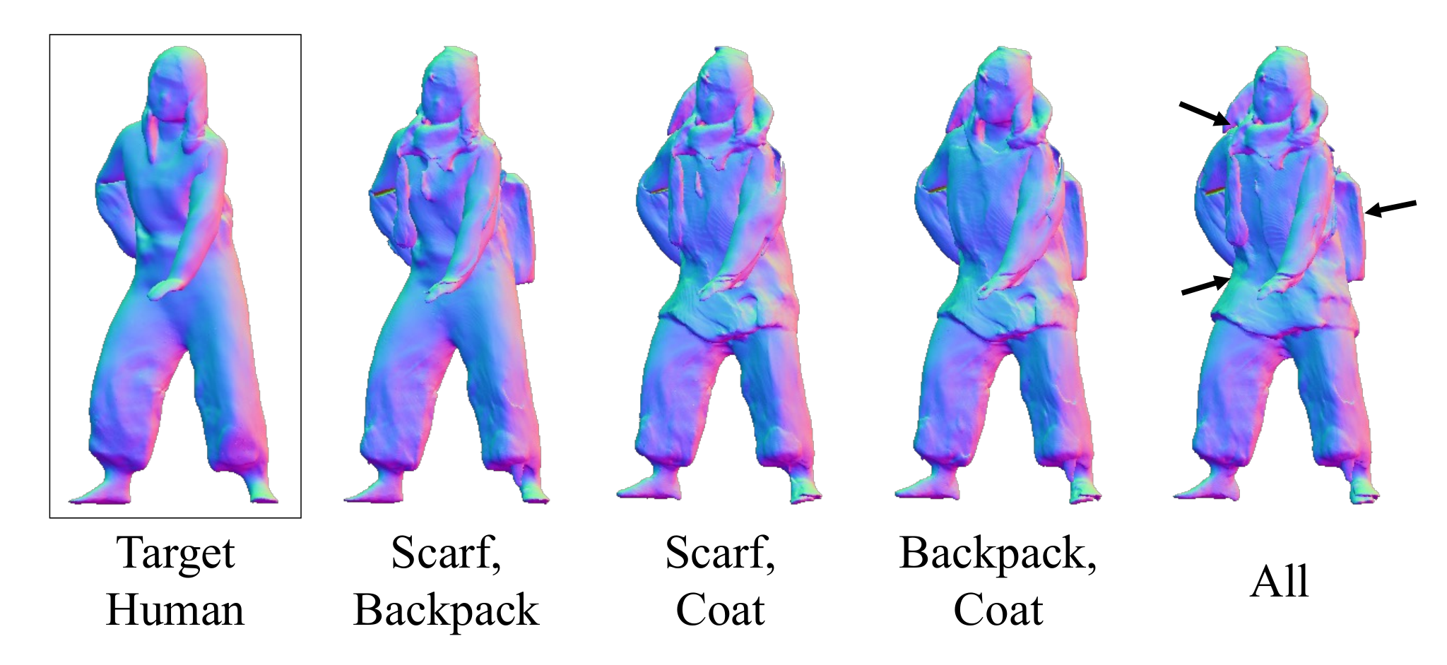
Composition of Multiple Objects. Fig. 8 shows that our system allows the composition of multiple objects. To add multiple objects, we use the latent code of each object and get the occupancy and the feature vector of objects. Using the normalized occupancy of multiple objects as weights, we calculate the weighted sum of feature vectors. The aggregated feature is then fed to the composition module along with the human feature to get the final composition output. Note that our dataset has no such sample with multiple objects.

Method	FID	User Preference
gDNA (w/ object)	41.71	43.6%
Arith. gDNA (w/ object)	73.81	13.6%
Ours (Naive composition)	55.29	22.4%
Ours	51.03	100% - (above)

Table 1: Quantitative evaluation of the importance of compositional modeling. User preference score reflects the frequency with which participants of our perceptual study favored each method over ours.

5.3 Comparison with SOTA

Since our method is the first generative model for compositing humans and objects, there is no direct competitor, and comparison with the previous non-compositional model such as gDNA is non-trivial. To make the assessment possible at our best, we consider a specific scenario where a user wants to create samples with a specific object category, being the backpack here. To provide such controllability on gDNA, we first extend the gDNA model with our dataset. Note that, in this evaluation, we use the same dataset $\mathbf{S}_{th}$ , $\mathbf{S}_{sh}$ , $\mathbf{S}_{sh+bp}$ for training both our model and gDNA.

Extending gDNA for Composition. We train gDNA model using the public code with our datasets. Both human-only outputs and the ones with a backpack can be sampled from the trained model. To intentionally generate outputs with a backpack, we search the latent codes associated with the training samples with backpacks and fit a gaussian from which we can perform a sampling. We denote this baseline method as ‘gDNA (w/ object)’.

The second possible extension of gDNA is based on the arithmetic operation among gDNA’s latent codes, which is widely used for GAN-based image manipulation radford2015unsupervised. We found that gDNA’s original framework allows some level of composition by adding or subtracting the latent codes. Specifically, we choose a latent code $\mathbf{z}_{sh}^{*}$ for the source human without a backpack and another latent code $\mathbf{z}_{sh+bp}^{*}$ for the source human with the backpack. We simply take their subtraction $\mathbf{z}_{bp}=\mathbf{z}_{sh+bp}^{*}-\mathbf{z}_{sh}^{*}$ , which can be considered as a residual for the backpack. We found that composition can be performed by adding this residual to another human’s latent code, that is $\mathbf{z}_{bp}+\mathbf{z}_{th}$ . We denote this baseline method as ‘Arith. gDNA (w/ object)’.

Qualitative Comparison with User Study. The visual comparison between ours and the extended gDNAs is shown in Fig. 9. In the first row, we show random samples generated from ‘gDNA (w/ object)’. Since the human scans with the backpack are only of the source human’s (other samples from $\mathbf{S}_{th}$ do not have any backpack), the generated outputs lack shape variety for the human part, producing always the source human’s identity. In the second row of Fig. 9, backpacks are added to novel identities; however, the method suffers from lack of details on both humans and objects. In contrast, the outputs of our method shown in the last row show strong generalization by creating diverse human identities with naturally attached detailed objects.

To further validate this comparison, we perform a user test (A/B test) on CloudResearch Connect. We render samples from three viewpoints (same views for all) and show ours with each baseline (A/B examples) in a random order to each subject. Each subject answers 5 questions per baseline by choosing more authentic 3D human samples. The data was collected from 50 subjects. The results are shown in the “User Preference” column in Tab. 1. As shown, our methods are preferred over extended gDNA baselines. Moreover, to confirm the diversity of identities in our method and ‘gDNA (w/ object)’, 50 subjects were shown the rendering of the source human and were asked to choose samples that don’t resemble the source human. Samples of our method were chosen by 92.4%, indicating that ‘gDNA (w/ object)’ suffers to generate novel identities with a backpack.

Quantiative Evaluation via FID. To evaluate the generation quality of our method, we compare Fréchet Inception Distance (FID) between the 2D normal renderings of the test dataset $\mathbf{S}_{unseen+bp}$ and the generated outputs, following chen2022gdna. The result is shown in Tab. 1. ‘gDNA (w/ object)’ has a relatively better score than ours, due to the fact that it only samples 3D humans around $\mathbf{S}_{sh+bp}$ , which are always close to the GT samples. A more fair comparison is between ours and ‘Arith. gDNA (w/ object)’, where both approaches try to attach the backpack to novel identities. Our method significantly outperforms this baseline.

Method	Pred-to-Scan ${\downarrow}$	Scan-to-Pred ${\downarrow}$
gDNA	0.0162	0.0190
gDNA(w/ object)	0.0218	0.0112
Ours	0.0116	0.0099

Table 2: Fitting accuracy comparison with the SOTA method chen2022gdna.

Performance on Fitting. We evaluate the expressiveness of our model by fitting it to unseen scans with objects. As a baseline, we consider gDNA chen2022gdna as it demonstrates better fitting results on 3D clothed human scans over other SOTA methods palafox2021npms; corona2021smplicit. Besides the original gDNA trained with $\mathbf{S}_{th}$ , we also consider gDNA trained with $\mathbf{S}_{th}$ , $\mathbf{S}_{sh}$ and $\mathbf{S}_{sh+bp}$ (‘gDNA (w/ object)’) to enable fitting of the object part. We use scans with backpacks from Renderpeople²² 2 RenderPeople was downloaded, accessed, and used in this research exclusively at SNU. renderpeople and captured dataset $\mathbf{S}_{unseen+bp}$ for fitting comparison.

As shown in Tab. 2, our method reports better fitting accuracy than the baselines. Our method effectively fits the geometry of both humans and objects while baselines only reconstruct either the human part or the object part as shown in Fig. 10. Moreover, since our method separately models humans and objects, it enables the high-quality removal of objects after fitting.

5.4 Ablation Study

Neural Composition. Our system provides two ways of extracting the final composition output. One is by using $o_{comp}$ : neural composition, and the other is by using the maximum value between $o_{h}$ and $o_{o}$ of queried points: naive composition. We verify the necessity of using neural composition in order to generate high-quality outputs of humans with objects. Compared to naive composition, neural composition remarkably reduces the artifacts induced by the imperfect fitting of the source human, resulting in lower FID values (Tab. 1). Qualitative comparison is presented in Fig. 11.

6 Discussion

We present a novel framework for learning a compositional generative model of humans and objects. Our compositional generative model provides separate control over the human part and the object part. To train our compositional model without manual annotation for the object geometries, we propose to leverage 3D scans of a single person with and without objects. Our results show that the learned generative model for the object part can be authentically transferred to novel human identities.

Limitations and Future Work. While our approach is general and supports diverse objects, decomposing thin layers of clothing in an unsupervised manner remains a challenge due to the limited precision of 3D scans. Extending our approach to modeling from RGB images is also an exciting research direction for future work.

Acknowledgements: This work of H. Joo and T. Kim was supported by SNU Creative-Pioneering Researchers Program and IITP grant funded by the Korean government (MSIT) [NO.2021-0-01343 and No.2022-0-00156]

References

(1) Thiemo Alldieck, Marcus Magnor, Bharat Lal Bhatnagar, Christian Theobalt, and Gerard Pons-Moll. Learning to reconstruct people in clothing from a single rgb camera. In CVPR, 2019.
(2) Thiemo Alldieck, Marcus Magnor, Weipeng Xu, Christian Theobalt, and Gerard Pons-Moll. Video based reconstruction of 3d people models. In CVPR, 2018.
(3) Thiemo Alldieck, Hongyi Xu, and Cristian Sminchisescu. imghum: Implicit generative models of 3d human shape and articulated pose. In ICCV, 2021.
(4) Dragomir Anguelov, Praveen Srinivasan, Daphne Koller, Sebastian Thrun, Jim Rodgers, and James Davis. Scape: shape completion and animation of people. In TOG. 2005.
(5) Samaneh Azadi, Deepak Pathak, Sayna Ebrahimi, and Trevor Darrell. Compositional gan: Learning image-conditional binary composition. IJCV, 2020.
(6) Bharat Lal Bhatnagar, Garvita Tiwari, Christian Theobalt, and Gerard Pons-Moll. Multi-garment net: Learning to dress 3d people from images. In ICCV, 2019.
(7) Sourav Biswas, Kangxue Yin, Maria Shugrina, Sanja Fidler, and Sameh Khamis. Hierarchical neural implicit pose network for animation and motion retargeting. arXiv preprint arXiv:2112.00958, 2021.
(8) Federica Bogo, Angjoo Kanazawa, Christoph Lassner, Peter Gehler, Javier Romero, and Michael J. Black. Keep it smpl: Automatic estimation of 3d human pose and shape from a single image. In ECCV, 2016.
(9) Mallikarjun BR, Ayush Tewari, Xingang Pan, Mohamed Elgharib, and Christian Theobalt. gcorf: Generative compositional radiance fields. 3DV, 2022.
(10) Zhe Cao, Tomas Simon, Shih-En Wei, and Yaser Sheikh. Realtime multi-person 2d pose estimation using part affinity fields. In CVPR, 2017.
(11) Eric R Chan, Connor Z Lin, Matthew A Chan, Koki Nagano, Boxiao Pan, Shalini De Mello, Orazio Gallo, Leonidas J Guibas, Jonathan Tremblay, Sameh Khamis, et al. Efficient geometry-aware 3d generative adversarial networks. In CVPR, 2022.
(12) Angel X Chang, Thomas Funkhouser, Leonidas Guibas, Pat Hanrahan, Qixing Huang, Zimo Li, Silvio Savarese, Manolis Savva, Shuran Song, Hao Su, et al. Shapenet: An information-rich 3d model repository. arXiv preprint arXiv:1512.03012, 2015.
(13) Xu Chen, Tianjian Jiang, Jie Song, Jinlong Yang, Michael J Black, Andreas Geiger, and Otmar Hilliges. gdna: Towards generative detailed neural avatars. In CVPR, 2022.
(14) Xu Chen, Yufeng Zheng, Michael J Black, Otmar Hilliges, and Andreas Geiger. Snarf: Differentiable forward skinning for animating non-rigid neural implicit shapes. In ICCV, 2021.
(15) Zhiqin Chen and Hao Zhang. Learning implicit fields for generative shape modeling. In CVPR, 2019.
(16) Enric Corona, Albert Pumarola, Guillem Alenya, Gerard Pons-Moll, and Francesc Moreno-Noguer. Smplicit: Topology-aware generative model for clothed people. In CVPR, 2021.
(17) Boyang Deng, John P Lewis, Timothy Jeruzalski, Gerard Pons-Moll, Geoffrey Hinton, Mohammad Norouzi, and Andrea Tagliasacchi. Nasa neural articulated shape approximation. In ECCV, 2020.
(18) Prafulla Dhariwal and Alexander Nichol. Diffusion models beat gans on image synthesis. In NeurIPS, 2021.
(19) Yao Feng, Jinlong Yang, Marc Pollefeys, Michael J. Black, and Timo Bolkart. Capturing and animation of body and clothing from monocular video. In SIGGRAPH Asia, 2022.
(20) Ian Goodfellow, Jean Pouget-Abadie, Mehdi Mirza, Bing Xu, David Warde-Farley, Sherjil Ozair, Aaron Courville, and Yoshua Bengio. Generative adversarial nets. In NeurIPS, 2014.
(21) Ian Goodfellow, Jean Pouget-Abadie, Mehdi Mirza, Bing Xu, David Warde-Farley, Sherjil Ozair, Aaron Courville, and Yoshua Bengio. Generative adversarial networks. Communications of the ACM, 2020.
(22) Amos Gropp, Lior Yariv, Niv Haim, Matan Atzmon, and Yaron Lipman. Implicit geometric regularization for learning shapes. In ICML. 2020.
(23) Jonathan Ho, Chitwan Saharia, William Chan, David J Fleet, Mohammad Norouzi, and Tim Salimans. Cascaded diffusion models for high fidelity image generation. JMLR, 2022.
(24) Fangzhou Hong, Mingyuan Zhang, Liang Pan, Zhongang Cai, Lei Yang, and Ziwei Liu. Avatarclip: Zero-shot text-driven generation and animation of 3d avatars. TOG, 2022.
(25) Xun Huang and Serge Belongie. Arbitrary style transfer in real-time with adaptive instance normalization. In ICCV, 2017.
(26) Boyi Jiang, Yang Hong, Hujun Bao, and Juyong Zhang. Selfrecon: Self reconstruction your digital avatar from monocular video. In CVPR, 2022.
(27) Boyi Jiang, Juyong Zhang, Yang Hong, Jinhao Luo, Ligang Liu, and Hujun Bao. Bcnet: Learning body and cloth shape from a single image. In ECCV, 2020.
(28) Hanbyul Joo, Tomas Simon, and Yaser Sheikh. Total capture: A 3d deformation model for tracking faces, hands, and bodies. In CVPR, 2018.
(29) Tero Karras, Timo Aila, Samuli Laine, and Jaakko Lehtinen. Progressive growing of gans for improved quality, stability, and variation. ICLR, 2017.
(30) Tero Karras, Samuli Laine, and Timo Aila. A style-based generator architecture for generative adversarial networks. In CVPR, 2019.
(31) Tero Karras, Samuli Laine, Miika Aittala, Janne Hellsten, Jaakko Lehtinen, and Timo Aila. Analyzing and improving the image quality of stylegan. In CVPR, 2020.
(32) Michael Kazhdan and Hugues Hoppe. Screened poisson surface reconstruction. TOG, 2013.
(33) Diederik P Kingma and Max Welling. Auto-encoding variational bayes. ICLR, 2013.
(34) Junxuan Li, Shunsuke Saito, Tomas Simon, Stephen Lombardi, Hongdong Li, and Jason Saragih. Megane: Morphable eyeglass and avatar network. In CVPR, 2023.
(35) Chen-Hsuan Lin, Ersin Yumer, Oliver Wang, Eli Shechtman, and Simon Lucey. St-gan: Spatial transformer generative adversarial networks for image compositing. In CVPR, 2018.
(36) Matthew Loper, Naureen Mahmood, Javier Romero, Gerard Pons-Moll, and Michael J. Black. SMPL: A skinned multi-person linear model. SIGGRAPH Asia, 2015.
(37) Qianli Ma, Jinlong Yang, Anurag Ranjan, Sergi Pujades, Gerard Pons-Moll, Siyu Tang, and Michael J Black. Learning to dress 3d people in generative clothing. In CVPR, 2020.
(38) Qianli Ma, Jinlong Yang, Siyu Tang, and Michael J. Black. The power of points for modeling humans in clothing. In ICCV, 2021.
(39) Lars Mescheder, Michael Oechsle, Michael Niemeyer, Sebastian Nowozin, and Andreas Geiger. Occupancy networks: Learning 3d reconstruction in function space. In CVPR, 2019.
(40) Marko Mihajlovic, Shunsuke Saito, Aayush Bansal, Michael Zollhoefer, and Siyu Tang. Coap: Compositional articulated occupancy of people. In CVPR, 2022.
(41) Marko Mihajlovic, Yan Zhang, Michael J Black, and Siyu Tang. Leap: Learning articulated occupancy of people. In CVPR, 2021.
(42) Ben Mildenhall, Pratul P Srinivasan, Matthew Tancik, Jonathan T Barron, Ravi Ramamoorthi, and Ren Ng. Nerf: Representing scenes as neural radiance fields for view synthesis. In ECCV, 2020.
(43) Richard A Newcombe, Shahram Izadi, Otmar Hilliges, David Molyneaux, David Kim, Andrew J Davison, Pushmeet Kohi, Jamie Shotton, Steve Hodges, and Andrew Fitzgibbon. Kinectfusion: Real-time dense surface mapping and tracking. In ISMAR, 2011.
(44) Thu Nguyen-Phuoc, Chuan Li, Lucas Theis, Christian Richardt, and Yong-Liang Yang. Hologan: Unsupervised learning of 3d representations from natural images. In ICCV, 2019.
(45) Michael Niemeyer and Andreas Geiger. Giraffe: Representing scenes as compositional generative neural feature fields. In CVPR, 2021.
(46) Atsuhiro Noguchi, Xiao Sun, Stephen Lin, and Tatsuya Harada. Neural articulated radiance field. In ICCV, 2021.
(47) Julian Ost, Fahim Mannan, Nils Thuerey, Julian Knodt, and Felix Heide. Neural scene graphs for dynamic scenes. In CVPR, 2021.
(48) Pablo Palafox, Aljaž Božič, Justus Thies, Matthias Nießner, and Angela Dai. Npms: Neural parametric models for 3d deformable shapes. In ICCV, 2021.
(49) Jeong Joon Park, Peter Florence, Julian Straub, Richard Newcombe, and Steven Lovegrove. Deepsdf: Learning continuous signed distance functions for shape representation. In CVPR, 2019.
(50) Georgios Pavlakos, Vasileios Choutas, Nima Ghorbani, Timo Bolkart, Ahmed A. A. Osman, Dimitrios Tzionas, and Michael J. Black. Expressive body capture: 3D hands, face, and body from a single image. In CVPR, 2019.
(51) Alec Radford, Luke Metz, and Soumith Chintala. Unsupervised representation learning with deep convolutional generative adversarial networks. ICLR, 2016.
(52) Renderpeople, 2018. https://renderpeople.com/3d-people.
(53) Robin Rombach, Andreas Blattmann, Dominik Lorenz, Patrick Esser, and Björn Ommer. High-resolution image synthesis with latent diffusion models. In CVPR, 2022.
(54) Shunsuke Saito, Zeng Huang, Ryota Natsume, Shigeo Morishima, Angjoo Kanazawa, and Hao Li. Pifu: Pixel-aligned implicit function for high-resolution clothed human digitization. In ICCV, 2019.
(55) Shunsuke Saito, Tomas Simon, Jason Saragih, and Hanbyul Joo. Pifuhd: Multi-level pixel-aligned implicit function for high-resolution 3d human digitization. In CVPR, 2020.
(56) Shunsuke Saito, Jinlong Yang, Qianli Ma, and Michael J Black. Scanimate: Weakly supervised learning of skinned clothed avatar networks. In CVPR, 2021.
(57) Johannes L Schonberger and Jan-Michael Frahm. Structure-from-motion revisited. In CVPR, 2016.
(58) Katja Schwarz, Yiyi Liao, Michael Niemeyer, and Andreas Geiger. Graf: Generative radiance fields for 3d-aware image synthesis. NeurIPS, 2020.
(59) Vincent Sitzmann, Julien Martel, Alexander Bergman, David Lindell, and Gordon Wetzstein. Implicit neural representations with periodic activation functions. NeurIPS, 2020.
(60) Jascha Sohl-Dickstein, Eric A. Weiss, Niru Maheswaranathan, and Surya Ganguli. Deep unsupervised learning using nonequilibrium thermodynamics. In ICML, 2015.
(61) Shih-Yang Su, Frank Yu, Michael Zollhöfer, and Helge Rhodin. A-nerf: Articulated neural radiance fields for learning human shape, appearance, and pose. NeurIPS, 2021.
(62) Garvita Tiwari, Nikolaos Sarafianos, Tony Tung, and Gerard Pons-Moll. Neural-gif: Neural generalized implicit functions for animating people in clothing. In ICCV, 2021.
(63) Yi-Hsuan Tsai, Xiaohui Shen, Zhe Lin, Kalyan Sunkavalli, Xin Lu, and Ming-Hsuan Yang. Deep image harmonization. In CVPR, 2017.
(64) Raquel Vidaurre, Igor Santesteban, Elena Garces, and Dan Casas. Fully convolutional graph neural networks for parametric virtual try-on. In CGF, 2020.
(65) Shaofei Wang, Katja Schwarz, Andreas Geiger, and Siyu Tang. Arah: Animatable volume rendering of articulated human sdfs. In ECCV, 2022.
(66) Ziyan Wang, Timur Bagautdinov, Stephen Lombardi, Tomas Simon, Jason Saragih, Jessica Hodgins, and Michael Zollhofer. Learning compositional radiance fields of dynamic human heads. In CVPR, 2021.
(67) Qianyi Wu, Xian Liu, Yuedong Chen, Kejie Li, Chuanxia Zheng, Jianfei Cai, and Jianmin Zheng. Object-compositional neural implicit surfaces. In ECCV, 2022.
(68) Donglai Xiang, Timur Bagautdinov, Tuur Stuyck, Fabian Prada, Javier Romero, Weipeng Xu, Shunsuke Saito, Jingfan Guo, Breannan Smith, Takaaki Shiratori, et al. Dressing avatars: Deep photorealistic appearance for physically simulated clothing. TOG, 2022.
(69) Yiheng Xie, Towaki Takikawa, Shunsuke Saito, Or Litany, Shiqin Yan, Numair Khan, Federico Tombari, James Tompkin, Vincent Sitzmann, and Srinath Sridhar. Neural fields in visual computing and beyond. In CGF, 2022.
(70) Yuliang Xiu, Jinlong Yang, Dimitrios Tzionas, and Michael J Black. Icon: implicit clothed humans obtained from normals. In CVPR, 2022.
(71) Hongyi Xu, Eduard Gabriel Bazavan, Andrei Zanfir, William T Freeman, Rahul Sukthankar, and Cristian Sminchisescu. Ghum & ghuml: Generative 3d human shape and articulated pose models. In CVPR, 2020.
(72) Yang Xue, Yuheng Li, Krishna Kumar Singh, and Yong Jae Lee. Giraffe hd: A high-resolution 3d-aware generative model. In CVPR, 2022.
(73) Bangbang Yang, Yinda Zhang, Yinghao Xu, Yijin Li, Han Zhou, Hujun Bao, Guofeng Zhang, and Zhaopeng Cui. Learning object-compositional neural radiance field for editable scene rendering. In ICCV, 2021.
(74) Hong-Xing Yu, Leonidas J. Guibas, and Jiajun Wu. Unsupervised discovery of object radiance fields. In ICLR, 2022.
(75) Tao Yu, Zerong Zheng, Kaiwen Guo, Pengpeng Liu, Qionghai Dai, and Yebin Liu. Function4d: Real-time human volumetric capture from very sparse consumer rgbd sensors. In CVPR, 2021.
(76) Heming Zhu, Yu Cao, Hang Jin, Weikai Chen, Dong Du, Zhangye Wang, Shuguang Cui, and Xiaoguang Han. Deep fashion3d: A dataset and benchmark for 3d garment reconstruction from single images. In ECCV, 2020.
(77) Jun-Yan Zhu, Philipp Krahenbuhl, Eli Shechtman, and Alexei A Efros. Learning a discriminative model for the perception of realism in composite images. In ICCV, 2015.

Appendix A Implementation details

A.1 Network Architectures

Latent codes assigned to each scan, $\mathbf{z}_{th}$ , $\mathbf{z}_{sh}$ , and $\mathbf{z}_{o}$ are 64-dimensional. For $\mathbf{z}_{o}$ , we use its first 5 bits to encode the object category via one-hot encoding and optimize only the last 59 bits during training. The generator $G$ of the human module and the object module generates the $256\times 256\times 64$ feature image from a constant vector of size $256\times 16\times 16$ via 4 layers of (bilinear upsampler with a scale factor of 2, 2D convolution of kernel size 3 and stride 1, adaIN for conditioning the generator with the latent code $\mathbf{z}$ , and leaky ReLU activations). The $256\times 256\times 64$ output feature image is split into one $256\times 256\times 32$ and two $256\times 128\times 32$ to form a tri-plane feature map. Note that the feature map is 128-dimensional along z-axis and 256-dimensional along other axes. The decoder for predicting the occupancy of the human module and the object module is a multi-layer perceptron having the intermediate neuron size of (256, 256, 256, 229, 1) with skip connection from the input features to the 4th layer and nonlinear activations of softplus with $\beta=100$ except for the last layer that uses sigmoid. As an input, it takes the Cartesian coordinates in canonical space which are encoded using a positional encoding with 4 frequency components, and the 32-dimensional feature queried from the generated tri-plane. The decoder for predicting SDF of the human module has the same architecture as the decoder for predicting the occupancy, except that it has no activations for the last layer. The decoder for predicting the occupancy of the composition module has the same architecture as the decoders for predicting the occupancy of other modules. However, instead of taking in the feature from the generated tri-plane as an input, it takes in the intermediate latent feature vectors before the last layer of the decoders for predicting the occupancy of the human module and object module, which are 229-dimensional each.

Our deformation networks $D=(W,N)$ follow the architecture of the deformer of gDNA chen2022gdna. The skinning network $W$ is a multi-layer perceptron having the intermediate neuron size of (128, 128, 128, 128, 24) with nonlinear activations of softplus with $\beta=100$ , except for the last layer that uses softmax in order to get normalized skinning weights. As an input, it takes the Cartesian coordinates in canonical space and the latent code $\mathbf{z}\in\mathbb{R}^{64}$ of the training sample. The warping network $N$ is also a multi-layer perceptron having the intermediate neuron size of (128, 128, 128, 128, 3) with nonlinear activations of softplus. As an input, it takes the Cartesian coordinates in canonical space and the SMPL shape parameter $\beta\in\mathbb{R}^{10}$ of the training sample. The input Cartesian coordinates are passed to the last layer for the network to learn residual displacements.

A.2 Training Procedure

Our training consists of three stages. First, we train $\mathcal{M}_{th}$ and $\mathbf{z}_{th}$ with $\mathbf{S}_{th}$ with losses following chen2021snarf; chen2022gdna and additional losses to train the SDF network. The total loss $\mathcal{L}_{M_{th}}$ is as follows:

	$\displaystyle\mathcal{L}_{M_{th}}=\mathcal{L}_{th}+\lambda_{bone}\mathcal{L}_{bone}+\lambda_{joint}\mathcal{L}_{joint}+\lambda_{warp}\mathcal{L}_{warp}$		(23)
	$\displaystyle+\lambda_{reg\_th}\mathcal{L}_{reg\_th}+\mathcal{L}_{sdf}+\mathcal{L}_{nml}+\mathcal{L}_{igr}+\mathcal{L}_{bbox},$

where $\lambda_{warp}=10$ and $\lambda_{reg\_th}=10^{-3}$ . We set $\lambda_{bone}=1$ and $\lambda_{joint}=10$ only for the first epoch and 0 afterwards.

For the second stage, we train $\mathcal{M}_{sh}$ and $\mathbf{z}_{sh}$ with $\mathbf{S}_{sh}$ with the total loss $\mathcal{L}_{M_{th}}$ being,

\displaystyle\mathcal{L}_{M_{sh}}=\mathcal{L}_{sh}+\lambda_{reg\_sh}\mathcal{L}_{reg\_sh},

(24)

where $\lambda_{reg\_sh}=10^{-3}$ . As described in the main paper, since we initialize $D_{sh}$ with the pre-trained $D_{th}$ , additional guidance losses as in the first stage are not required. Note that since it is not our primary objective to model the detailed surface of the source human, we don’t utilize the hybrid modeling of occupancy and SDF for $\mathcal{M}_{sh}$ .

For the last stage, we train $\mathcal{M}_{o}$ , $\mathcal{M}_{comp}$ , $\mathbf{z}_{sh}$ , and $\mathbf{z}_{o}$ with the pre-trained $\mathcal{M}_{th}$ , $\mathcal{M}_{sh}$ and $\mathbf{z}_{th}$ frozen. As described in the main paper, $\mathbf{z}_{sh}$ for the last stage are re-initialized as the mean of $\mathbf{z}_{sh}$ after the second stage. The total loss $\mathcal{L}$ is as follows:

	$\displaystyle\mathcal{L}=\mathcal{L}_{comp}+\mathcal{L}_{o}+\lambda_{fit}\mathcal{L}_{fit}$		(25)
	$\displaystyle+\lambda_{reg\_sh}\mathcal{L}_{reg\_sh}+\lambda_{reg\_o}\mathcal{L}_{reg\_o},$

where $\lambda_{fit}=0.2$ , $\lambda_{reg\_sh}=50$ , and $\lambda_{reg\_sh}=10^{-3}$ .

We train each stage with the Adam optimizer with a learning rate of 0.001 without decay. All stages are trained for 300 epochs.

A.3 Inference

We generate the composited canonical shapes of general people with objects by random sampling $\mathbf{z}_{th}$ and $\mathbf{z}_{o}$ from the Gaussian distribution fitted to each set of latent codes. We then extract meshes using $o_{comp}$ with a resolution of $256^{3}$ . We finally repose the output mesh using the SMPL pose parameter with the learned skinning fields.

Appendix B Data

B.1 Acquisition

We collect 3D scans of the source human with and without objects using a system with synchronized and calibrated 8 Azure Kinects. We capture data 5FPS with the resolution of $2048\times 1536$ for the RGB cameras, and $1024\times 1024$ for the depth cameras. We perform image-based calibration using COLMAP schonberger2016structure and adjust the optimized camera extrinsics to real-world scale based on the corresponding depth maps. We apply KinectFusion newcombe2011kinectfusion with the code from the repository ³³ 3 https://github.com/andyzeng/tsdf-fusion-python to fuse the captured depth maps with the voxel resolution of 1.5mm. We reconstruct watertight meshes from the fused output using screened-poisson surface reconstruction kazhdan2013screened of depth 9. In order to obtain SMPL parameters for each captured scan, we use the multi-view extension of SMPLify Bogo2016 with the code from the repository ⁴⁴ 4 https://github.com/ZhengZerong/MultiviewSMPLifyX. For each scan, we render images from 18 viewpoints and detect 2D keypoints using OpenPose cao2017realtime, and apply the multi-view extension of SMPLify to estimate SMPL parameters for each scan.

B.2 Data Statistics

We use 180 samples for $\mathbf{S}_{sh}$ and 342 samples for $\mathbf{S}_{sh+o}$ . For $\mathbf{S}_{sh+o}$ , we consider 4 categories of objects: 5 backpacks (77 samples in total), 6 outwear (94 samples), 8 scarves (89 samples), and 6 hats (82 samples). For running the quantitative evaluation focused on backpacks, we use another set with 300 samples of the source human with 5 backpacks, denoted as $\mathbf{S}_{sh+bp}$ . To build a testing set for FID computation, we further capture 343 samples of 3 different unseen identities who wear unseen backpacks, denoted as $\mathbf{S}_{unseen+bp}$ . We also use 526 samples of THuman2.0 tao2021function4d for $\mathbf{S}_{th}$ .

Appendix C Discussion

Method	Chamfer ${\downarrow}$	P2S ${\downarrow}$	Normal ${\downarrow}$
Occ	0.0140	0.0169	0.0092
Occ & SDF	0.0098	0.0128	0.0074

Table 3: Quantitative evaluation of the significance of using the hybrid modeling of occupancy and SDF is presented.

C.1 Geometry Modeling with SDF

As mentioned in the main paper, we model detailed geometry by jointly predicting SDF together with the occupancy fields. We find that directly replacing the occupancy with the SDF leads to failures in canonicalization. Among the set of correspondences resulting from multiple initials for the root finding algorithm, previous work that uses occupancy representation chen2021snarf; chen2022gdna determines the final correspondence by choosing the point with the highest estimated occupancy. However, in the case of the SDF representation, we empirically find out that choosing the point by only utilizing the estimated SDF leads to poor canonicalization. Moreover, using a single initial by linearly combining the skinning weights of the nearest neighbor on the fitted SMPL mesh and the inverse bone transformations as in wang2022arah; jiang2022selfrecon also leads to incorrect canonicalization. Hence, we utilize a hybrid modeling of occupancy and SDF by leveraging the advantage of each representation. While directly supervising SDF on the surface normals, we select final correspondences and train the deformation networks using occupancy. For stable training, it is crucial to disable the backpropagation of gradients from the SDF head to the deformation networks and let only the occupancy head supervise them.

We verify the significance of predicting both occupancy and SDF over predicting only occupancy to generate outputs with higher frequency details. For each method, we reconstruct the ground truth data used for training with assigned latent codes. We compute the Chamfer distance and point-to-surface distance (P2S) between the ground truth and the reconstruction output. We also render 2D normal maps from fixed views and compute the L2 error (Normal). As demonstrated in Tab. 3, reconstruction outputs are improved when both occupancy and SDF are predicted. In Fig. 12 we show the qualitative comparison between samples generated via each method.

Appendix D Quantitative Evaluation Details

D.1 FID Computation

We compute FID score using the code from the repository⁵⁵ 5 https://github.com/mseitzer/pytorch-fid. For the test set, we render 2D normal maps in resolution $256^{2}$ of 343 samples in $\mathbf{S}_{unseen+bp}$ from 18 viewpoints, resulting in 6174 images. For each method, we generate 200 samples in random body sizes and poses of the $\mathbf{S}_{unseen+bp}$ and similarly render 2D normal maps in resolution $256^{2}$ from 18 viewpoints, resulting in 3600 images.

D.2 User Preference Study

We perform two user preference studies (A/B test) via CloudResearch Connect. The first study aims to validate the generation quality of our method over all baselines, and the second study aims to validate the generation diversity of our method over ‘gDNA (w/ object)’.

For the first user study, we show a sample generated with our method along with another sample generated with one of the baseline methods in random order. For each sample, we render 2D normal maps in resolution $256^{2}$ from 3 viewpoints. We ask 50 subjects to answer 5 A/B pairs per baseline by choosing the preferred sample with a more authentic shape. An example of a question is presented in Fig. 13

For the second user study, we only compare our method with the baseline, ‘gDNA (w/ object)’, with a different protocol. In this study, we similarly render the normal maps from 3 viewpoints from each method and additionally show an image of the source human along with the A/B pairs. Then, we request the observers to choose the sample that looks more different from the source human. The test is intended to see whether the methods can produce diverse human identities with objects, sufficiently different from the source human’s appearance. An example of a question is presented in Fig. 14. Similar to the first study, we ask 50 subjects to answer 5 A/B pairs by choosing the sample that better satisfies the question.

D.3 Fitting Comparison

For fitting our model to unseen scans with objects, we follow the fitting process of gDNA chen2022gdna. During fitting, we optimize the latent code for the human part, $\mathbf{z}_{h}$ , the latent code for the object part, $\mathbf{z}_{o}$ , and the SMPL shape parameter $\beta$ with other network frozen. We use $\mathcal{M}_{th}$ for the human module. We initialize $\mathbf{z}_{h}$ and $\mathbf{z}_{o}$ each with 8 randomly sampled codes from the Gaussian distribution fitted to each set of latent codes. $\beta$ is initialized with the obtained SMPL shape parameter during our data acquisition process. The loss $\mathcal{L}_{fitting}$ used for fitting raw scans is as follows:

	$\displaystyle\mathcal{L}_{fitting}=\mathcal{L}_{comp}+\lambda_{reg\_h}\mathcal{L}_{reg\_h}+\lambda_{reg\_o}\mathcal{L}_{reg\_o}$		(26)
	$\displaystyle\mathcal{L}_{comp}=BCE(o_{comp},o_{unseen})$		(27)
	$\displaystyle\mathcal{L}_{reg\_h}=\lVert\mathbf{z}_{h}\rVert$		(28)
	$\displaystyle\mathcal{L}_{reg\_o}=\lVert\mathbf{z}_{o}\rVert,$		(29)

where $\lambda_{reg\_h}=50$ and $\lambda_{reg\_o}=50$ . We optimize for 500 iterations using the Adam optimizer with a learning rate of 0.01 without any weight decay or learning rate decay. Of 8 fitted outputs, the one with the minimum bi-directional Chamfer distance to the target scan is chosen as the final output.

Appendix E Addtional Qualitative Results

Please refer to the supplementary video for additional qualitative results on individual control of the human and object modules, latent code interpolation, and composition of multiple objects.

NCHO: Unsupervised Learning for Neural 3D Composition of Humans and Objects