Impacts of symmetry energy slope on the oscillation frequencies of neutron stars with short-range correlation and admixed dark matterPreprint: APS/123-QED
Abstract
Oscillation modes of compact stars, in general, can serve as a fingerprint in determining the equation of state (EOS) of dense matter. In this study, we examine the impact of symmetry energy slope () on the oscillation frequencies of neutron stars (NSs) with nucleon-nucleon short range correlation (SRC) and admixed dark matter (DM) for the first time within the relativistic mean-field theory. By adjusting the , we revise the EOS and coupling parameters in light of the SRC and DM effects, and construct the new sets. The results reveal that NSs containing SRC and DM inside are more likely to satisfy the observational constraints, and we find that smaller exhibits larger fundamental non-radial and radial frequencies, and that the effect on Large Separation (LG) is also mainly concentrated in the low-mass region. Moreover, we update the linear relationship between the non-radial frequency and mean density, and we further give empirical relations between non-radial and radial frequencies and tidal deformability at different for 1.4 and 2. These findings will enable us to more effectively confine the NS EOSs, in turn, also provide a strategy to place constraints on the .
Keywords: Neutron stars; Nuclear astrophysics; Dark matter
I Introduction
As a class of very dense objects in astronomy, the description of matter at high density inside NSs has attracted a lot of attention from nuclear physics (Oertel et al. 2017), particle physics, and astrophysics (Jiang et al. 2020; Luo et al. 2022). However, given the non-perturbative nature of nuclear forces, we cannot derive the EOS directly from quantum chromodynamics (QCD). As a result, it is more common to construct NS EOSs from the microscopic first principles, such as (Epelbaum et al. 2009; Hammer et al. 2013; Holt et al. 2013; Tews et al. 2013; Lynn et al. 2016), or from the self-consistent phenomenological models, typical approaches like the Skyrme-Hartree-Fock (Stone and Reinhard 2007; Rikovska Stone et al. 2003; Dutra et al. 2012) and Gogny-Hartree-Fock (Loan et al. 2011; Gonzalez-Boquera et al. 2017), or from parameterization models (Read et al. 2009; Luo et al. 2022). These models are also strongly constrained by multi-messenger observations, including the recent series of discoveries of twice-solar-mass () NSs (Demorest et al. 2010; Fonseca et al. 2016; Arzoumanian et al. 2018; Antoniadis et al. 2013; Cromartie et al. 2020; Fonseca et al. 2021), the tidal deformability extracted from the binary NS merger event GW170817 (Abbott et al. 2019; Fasano et al. 2019), the simultaneous mass and radius measurements of the isolated PSR J00300451 by NICER (Neutron Star Interior Composition Explorer) (Miller et al. 2019; Riley et al. 2019) and the gravitational wave event GW190814 from the coalescence of a stellar-mass black hole and a mysterious compact star (Abbott et al. 2020). To some extent, these observations undoubtedly disprove certain EOSs, making it imperative to establish plausible ones that can describe the low density properties while meeting the observational constraints.
Nuclear microscopic scale nucleon-nucleon SRC (Arrington et al. 2012; degli Atti 2015; Hen et al. 2017) and cosmic macroscopic size DM have proven to be relatively challenging issues. Several theoretical works have demonstrated that, in contrast to the free Fermi gas, the SRC originating from the strongly repulsive core of nuclear force and its tensor part leads to an appreciable depletion below the Fermi surface, with some nucleons occupying regions above the Fermi surface and giving rise to a high-momentum tail, as has been verified by experiments like (Rohe et al. 2004) and (Onderwater et al. 1998; Starink et al. 2000). Furthermore, the SRC effects also play an important role in nuclear physics (Panda et al. 2006; Sammarruca 2014; Cai and Li 2015; Hen et al. 2015a; Wang et al. 2017; Yang et al. 2019), such as allowing us to have a better understanding of the EMC effect (Weinstein et al. 2011; Hen et al. 2012) and to explain the neutrino oscillation measurements (Fields et al. 2013; Fiorentini et al. 2013) as well as density-dependent behavior of nuclear symmetry energy (Hen et al. 2015a). When it is extended to study NSs, tidal deformability (Souza et al. 2020a; Hong et al. 2022), mass-radius relations (Li et al. 2019; Lu et al. 2021; Lourenço et al. 2022) and cooling efficiency will all be affected (Souza et al. 2020b). For DM, many observations such as gravitational lensing, galaxy rotation curves, velocity dispersions, galaxy clusters and cosmic microwave background have predicted its existence (for a review, see (Bertone et al. 2005; Bertone and Hooper 2018; Buen-Abad et al. 2022)). Although there are many candidates for DM, the origin and properties remain a mystery, moreover, DM does not interact directly with normal matter, but it has a more pronounced gravitational effect on dense objects like NSs (Kouvaris and Tinyakov 2011), and play a important role in determining NS mass-radius relation (Quddus et al. 2020; Lourenço et al. 2022) and tidal deformability (Das et al. 2021; Das et al. 2020). Despite this, there is still little ongoing research to incorporate nucleon-nucleon SRC into the admixed DM NSs and to further examine their effects.
The symmetry energy and its slope play a crucial role in determining the equation of state of pure neutron matter, which involves determining the neutron skin thickness in neutron-rich matter, the dynamics of heavy-ion collisions, and also affects the structure and properties of NSs, helping us understand isospin asymmetry physics under extreme conditions. Given that characterizes the density dependence of the symmetry energy, it not only determines the behavior of high-density asymmetry nuclear matter but also directly affects the supernova, and even the production of heavy elements in nucleosynthesis. Moreover, its value remains large uncertain and still requires theoretical and experimental studies. Therefore, we choose the symmetry energy slope to study its effect on the properties of NSs under the background of short-range correlations and dark matter admixed. In the work (Kong et al. 2017) the authors used two different methods to deduce its range around MeV and MeV, respectively, while the latest study employs Bayesian analysis to estimate to be around MeV (Tang et al. 2021). Recently, a more accurate model-independent experiment PREX-2 reported very thick 208Pb neutron skin thickness () (Adhikari et al. 2021), and based on this result with taking into account the strong correlation between and , the work (Reed et al. 2021) extracted a up to MeV, a value that seriously challenges our understanding of neutron-rich matter near the nuclear saturation density and will further aggravate the uncertainty in . Additionally, as the oscillation frequency is highly dependent on the NS internal structure, it is possible to understand the internal physics by analyzing GW signals from compact star oscillations in addition to signals from binary NS mergers. The presence of any non-axisymmetric perturbation in NSs caused by dynamical instabilities, such as starquakes, magnetic reconfiguration, and rotating (Jones 2002), is known to cause non-radial oscillations and thus emission of gravitational waves. Furthermore, depending on the restoring force, they can be classified as fundamental -modes, gravity -modes, pure time -modes, pressure -modes, and rotational -modes (Kokkotas and Schutz 1992; Lau et al. 2010; Kokkotas and Schmidt 1999). It is well known that non-radial oscillations of NSs are also accompanied by radial oscillations (Passamonti et al. 2007), and although radial oscillations do not produce gravitational radiation directly, they can couple and further amplify it (Passamonti et al. 2006; Passamonti et al. 2007). Many excellent works have been carried out to investigate the radial and non-radial oscillations, for example, by studying the difference in the oscillation frequency caused by the different components inside a NS, it is possible to identify whether it is a hadronic, hybrid or quark star (Vaeth and Chanmugam 1992; Vásquez Flores and Lugones 2010; Flores et al. 2017; Ranea-Sandoval et al. 2018; Pereira et al. 2018; Sun et al. 2021; Jaikumar et al. 2021; Lau and Yagi 2021). Moreover, numerical relativistic simulations show that binary NSs merger to form a hypermassive NS may experience strong radial oscillations and radiate GWs at kHz (Bauswein et al. 2014; Takami et al. 2014), and the identification of quasi-periodic oscillations in giant flares caused by NS torsional oscillations can also help us to effectively constrain the NS crust properties (Sotani et al. 2012a; Sotani et al. 2012b; Sotani et al. 2018; Sotani et al. 2019).
Given the fact that the is still theoretically uncertain, and that the NS oscillation frequency is expected to detect in the near future with the upgrade of the observational devices (Perkins et al. 2021; Punturo et al. 2010; Dwyer et al. 2015), so it is necessary to establish a link between them, which will not only assist us in establishing a bridge between theory and observation to better constrain the EOSs, but also to infer the theoretical value of from frequency. In light of this, we introduce the nucleon-nucleon SRC in the interior of admixed DM neutron stars and rebuilt the EOSs that not only satisfy the properties of nuclear matter at saturation density, but also satisfy the constraints from multi-messenger observation. Based on this, we examine the impact of on the NS radial and non-radial oscillations, build their relationship and predict their frequency ranges.
This article is organized as follows: Section II provides a basic introduction to theoretical models of SRC and DM in NSs. Section III discusses in detail the parameter construction that meets the constraints from saturation nuclear behaviors and multi-messenger observations. Section IV is devoted to investigate the implication of on the NS oscillation frequency, and Section V provides a brief summary and remark. Finally, Appendix shows a comprehensive derivation of relativistic nucleon coupling parameters by incorporating the SRC effect.
II Relativistic mean field theory with Short-Range correlation and Dark Matter Admixed
In this paper, we adopt relativistic mean field theory (RMF) with model. Based on this framework, we absorb the SRC and introduce the DM to give the SRC-DM-revised RMF. In the mean-field approximation, the energy density and pressure are expressed as follows:
and
| (2) |
where and denote the nucleon and lepton degrees of freedom, and ,, correspond to the mass of . Coupling parameters need to be further revised by incorporating SRC and DM and the detailed analytical derivation have been attached in the Appendix. For DM component, here we adopt the lightest neutralino as the Fermi DM candidate with a mass of =200 GeV. Moreover, DM and nucleons do not interact directly but through coupled Higgs fields, with the following Lagrangian form (Panotopoulos and Lopes 2017a):
| (3) | |||||
where , denote the DM and Higgs field, and is the coupling strength between DM and Higgs field which usually takes values between 0.001 and 0.1, here we adopt the generally used value of 0.07 (Murakami and Wells 2001; Panotopoulos and Lopes 2017a). refers to the mass of the Higgs boson, which is 125 GeV. is the effective Yukawa coupling strength between nucleon and Higgs field, where is the Higgs vacuum expectation value with GeV and is the Higgs-nucleon formation factor. Based on the lattice computations, we choose the optimal value of as 0.3, which is not only consistent with theoretical result (Cline et al. 2013) but also satisfies the experimental constraints of PandaX-II (Tan et al. 2016), PandaX-4T (Meng et al. 2021) for the DM-nucleon scattering cross section.
Finally, we assume that the DM number density is about 1000 times lower than the number density of nucleons, and if we take the typical nuclear saturation number density fm-3, the calculated DM Fermi energy is about 0.033 GeV. Applying the mean field approximation, the effective mass of nucleons and DM and its scalar density are given as,
| (4) | |||
| (5) | |||
| (6) |
while the energy density and pressure of dark matter are
| (7) |
and
| (8) |
Both and in the Eqs. (1) and (2) depend directly on the momentum distribution of the nucleon in the mean-field approximation, and therefore also on the SRC. Recent theoretical and experimental studies indicate that the short-range correlation produces a single nucleon momentum distribution that approximately satisfies the distribution near the Fermi surface (Wang et al. 2017; Hen et al. 2015a; Cai and Li 2015). The functional form has been shown to provide a good fit to experimental data on nucleon momentum distributions, and it is insensitive to the specific details of the nucleon-nucleon interaction and the nuclear wave function, making it a versatile tool in the study of nucleon momentum distributions. The form can be applied in a range of contexts, including electron scattering experiments (Rohe et al. 2004; Onderwater et al. 1998; Starink et al. 2000). Although the parameterized model mentioned above can well characterize the high-momentum tail caused by nucleon short-range correlations and is consistent with experimental results, there is still one thing to point out that the correlation percentage between nucleons and the form of high-momentum distribution caused by SRCs still depend on the model, and different models also have their own advantages in characterizing SRC, for example, the Green’s function method Dickhoff and Van Neck 2008 provides a powerful framework for describing nucleon SRCs in nuclear systems, and can help to shed light on the physics underlying these phenomena. In contrast, the form has the advantage of portraying a high-momentum tail on the one hand in its simple form, and on the other hand, it can qualitatively give similar high-momentum tail calculated using microscopic self-consistent Green’s function (SCGF) theory (Rios et al. 2014; Rios 2020). Moreover, because of its simplicity, the form has also been widely used in understanding nuclear matter properties (Wang et al. 2017; Sammarruca 2014; Cai and Li 2015; Hen et al. 2015a; Wang et al. 2017; Guo et al. 2021) and NS prosperties (Souza et al. 2020a; Hong et al. 2022; Li et al. 2019; Lu et al. 2021; Lourenço et al. 2022).
For asymmetry nuclear matter, based on the microscopic theoretical model predicting an approximate linear correlation between isospin-asymmetry and single-nucleon distribution, we can express the nucleon momentum distribution in the following form:
| (9) |
| (10) |
where is the isospin-asymmetry, and and are the Fermi momentum and high-momentum cutoff, respectively. According to experiments with proton-knockout reactions utilizing megaelectron-energy electron beams, around of the nucleons have high momentum distribution (Subedi et al. 2008). Furthermore, the deuteron momentum distribution suggests that the cutoff should be around (Hen et al. 2015b; Hen et al. 2015a). In the next discussion, we take the cutoff to be 2.75, while taking high-momentum ratio to be typically 25%. Combining the normalization conditions, we can fix the values of , , and they are , , and respectively. After incorporating results into Eqs. (1) and (2), the SRC-revised energy density and pressure are derived as follows:
and
| (12) |
Then the total energy density and pressure, revised jointly by admixing DM as well as SRC, are expressed as
| (13) |
As a part of standard NS calculation scheme, in the NS outer crust, where the density is around , we employ the Baym-Pethick-Sutherland (BPS) EOS (Baym et al. 1971). For NS inner crust area with a density of , we adopt the polytropic parametrized EOSs of (Cai and Li 2016; Xu et al. 2009; Carriere et al. 2003), where and are related to the core-crust transition . In this study, we examine the possible weak interaction between DM and ordinary baryonic matter, which occurs via the exchange of Higgs bosons. When solving the hydrostatic Tolman-Oppenheimer-Volkoff (TOV) equation, they resemble the degrees of freedom of hyperons inside NSs, hence we can regard the mixed system of DM and baryonic matter as a single-fluid system. Adopting the static spherically symmetric space-time background given by
| (14) |
with solving the Einstein equation, we can derive the Tolman-Oppenheimer-Volkoff (TOV) equation (Oppenheimer and Volkoff 1939)
| (15) |
| (16) |
in which the corresponding metric functions express as
| (17) |
| (18) |
Then with the beta equilibrium and charge conservation condition, the NS mass and radius can be determined.
III The construction of parameters
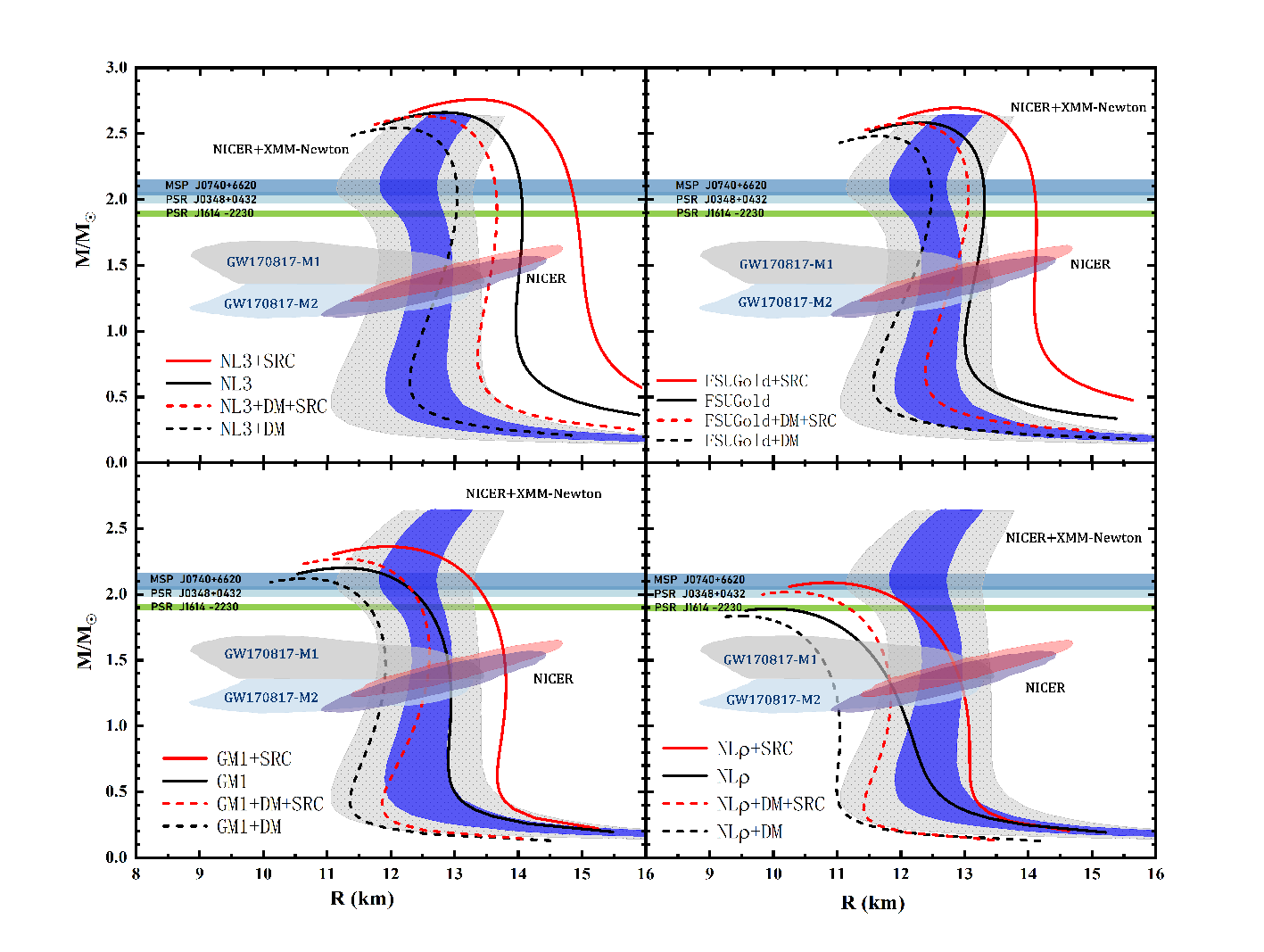
To better visualize the implications of SRC and DM on NSs, we choose four extensively used parameter sets to characterize the NS mass-radius relation, namely NL3 (Lalazissis et al. 1997), FSUGold (Todd-Rutel and Piekarewicz 2005), GM1 (Glendenning and Moszkowski 1991) and NL (Liu et al. 2002), as these sets can provide a good description of the properties of ground state nuclei and can be extrapolated to study standard NS matter. Moreover, as we mentioned before after the introduction of SRC in the mean field, in addition to the revisions of energy density and pressure, the coupling parameters between nucleons also need to be revised accordingly. The revised results are shown in Fig.1, where the black solid line indicates the mass-radius curve obtained from the original version, while the red solid line indicates the result of SRC effect, which makes the EOSs stiffer due to the additional correlation effect, being consistent with the conclusions from (Souza et al. 2020a; Lu et al. 2021). The black dashed line indicates the case of admixed DM, and it can be found that, compared to the original parameters, the introduction of DM substantially softens the EOS. To further compare with the astronomical observations, the constraints from different groups are attached to the figure, where the three horizontal light-colored bars indicate the three massive NSs (Demorest et al. 2010; Arzoumanian et al. 2018; Antoniadis et al. 2013; Cromartie et al. 2020; Fonseca et al. 2021), the middle elliptical shaded region indicates the constraints given by GW170817 (Abbott et al. 2017; Abbott et al. 2018; Annala et al. 2018; Most et al. 2018; De et al. 2018) and NICER (Miller et al. 2019; Riley et al. 2019; Miller et al. 2021), the vertical long shaded region indicates the mass-radius constraint given by NICER in conjunction with XMM-Newton through Bayesian analysis (Riley et al. 2021; Miller et al. 2021), in which the blue and gray region represent the 75% and 90% confidence intervals, respectively. Unfortunately, considering the SRC alone would largely increase the radius of NSs and thus make it easier to deviate from the astronomical constraints, as in the case of parameter NL3 and FSUGold, while considering admixed DM alone would make the EOSs excessively soft, as in the case of parameter NL. If the effects of both SRC and DM are considered inside the NSs, as shown by the red dotted line, their complementary mechanism makes the EOS curves easier to satisfy the observational constraints. Although we cannot draw an absolute conclusion from this due to the model dependence of the parameters, all four parameter sets support our conclusion of having both SRC and DM effects in the NS interior. Moreover, the SRC and admixed DM exhibit similar effects on the mass-radius curves for all four sets, and in view of this, here we have chosen only GM1 for the next discussion. The values are shown in Table I, where the first column is the original version for GM1 and the second column is the SRC and DM revised version (GM1+SD). By adjusting the range of while maintaining the other saturation properties, we investigate the impact of on the modified version. Such an approach keep the isoscalar nature unchanged and can satisfy the properties at the saturation density, and has been used in many works (Souza et al. 2020a; Hornick et al. 2018). We extract located around 5090 MeV within a relatively credible interval based on previous experimental and theoretical studies, and its corresponding modified versions (GM1+SD+L) are shown in the second half of the Table I.
| GM1 | GM1+SD | GM1+SD+L50 | GM1+SD+L60 | GM1+SD+L70 | GM1+SD+L80 | GM1+SD+L90 | |
| 939 | 939 | 939 | 939 | 939 | 939 | 939 | |
| 512 | 512 | 512 | 512 | 512 | 512 | 512 | |
| 783 | 783 | 783 | 783 | 783 | 783 | 783 | |
| 770 | 770 | 770 | 770 | 770 | 770 | 770 | |
| 0.153 | 0.153 | 0.153 | 0.153 | 0.153 | 0.153 | 0.153 | |
| 300 | 300 | 300 | 300 | 300 | 300 | 300 | |
| 0.70 | 0.70 | 0.70 | 0.70 | 0.70 | 0.70 | 0.70 | |
| 16.3 | 16.3 | 16.3 | 16.3 | 16.3 | 16.3 | 16.3 | |
| 32.5 | 32.5 | 32.5 | 32.5 | 32.5 | 32.5 | 32.5 | |
| 94 | 94 | 50 | 60 | 70 | 80 | 90 | |
| 8.910 | 9.321 | 9.321 | 9.321 | 9.321 | 9.321 | 9.321 | |
| 10.610 | 9.645 | 9.645 | 9.645 | 9.645 | 9.645 | 9.645 | |
| 8.196 | 13.566 | 14.934 | 14.587 | 14.263 | 13.960 | 13.675 | |
| 0.0029 | 0.0029 | 0.004 | 0.004 | 0.004 | 0.004 | 0.004 | |
| -0.001 | -0.001 | -0.003 | -0.003 | -0.003 | -0.003 | -0.003 | |
| 0 | 0.002 | 0.011 | 0.009 | 0.007 | 0.005 | 0.003 |
As a next step, we need to decide a key question: whether the sets constructed by different are able to describe empirical properties at low densities while also fulfilling constraints from multi-messenger observations? To this end, we have calculated the binding energy per nucleon (E/A) for symmetry nuclear matter (SNM) and pure neutron matter (PNM), as shown in Fig.2. The different color curves in the upper part indicate different for PNM, in which below the saturation number density (corresponding to the black vertical dashed line), the smaller gives a relatively large E/A, while the opposite is true above , and these results are in agreement with (Wu et al. 2021). Furthermore, in order to constrain the PNM behavior at subsaturation density, we adopt the given in (Tews et al. 2013), which presents next-to-next-to-next-to-leading order (N3LO) in the chiral expansion based on potentials developed by Epelbaum, Glckle and Meißner (EGM). As shown in the light green area (the lower right corner corresponds to the enlarged version), our revised parameters are largely in compliance with the constraints. Furthermore, it can be seen that is more supportive of smaller . The blue line shows the E/A for SNM, which, unlike PNM, is clearly independent of a specific and has a minimum value at , corresponding to the most stable ground state, of about -16 MeV.
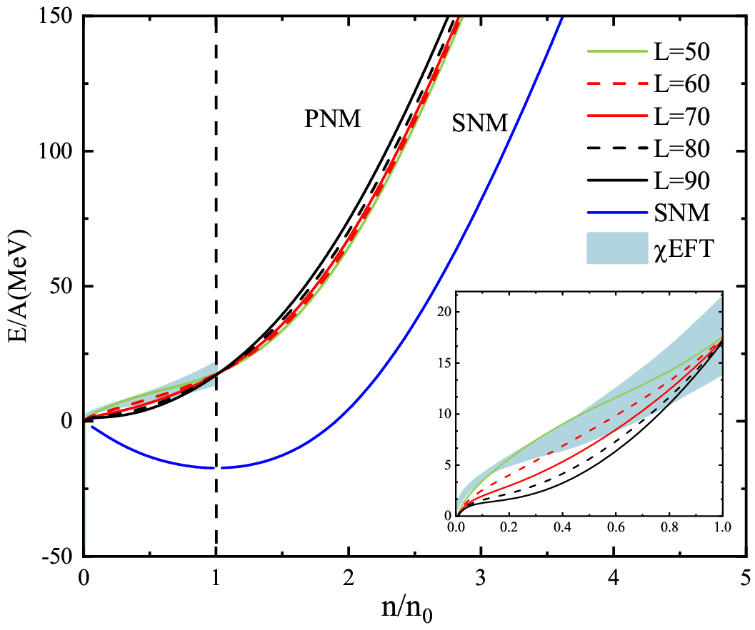
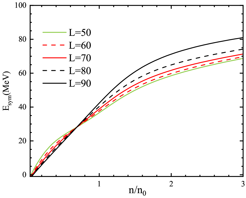
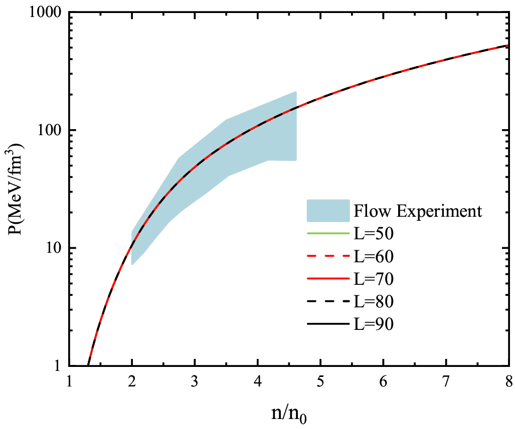
Fig.3 shows the symmetry energy as a function of density for different . As can be seen, with a smaller have a lower (higher) value than those with a larger at (), similar behavior is observed in (Hu et al. 2020; Wu et al. 2021). Fig.4 gives the pressure of SNM, and we includes the experimental constraints obtained from collective flow data in heavy-ion collisions which are often used to constrain the EOS of SNM (Huang et al. 2020; Cavagnoli et al. 2011). The enclosed area represents experimental data according to (Danielewicz et al. 2002), and our result is in line with this constraint.
Apart from that, reasonable parameters also need to satisfy the constraints from multi-messenger observations, including being able to generate massive NSs, meeting the mass-radius constraint derived from NICER+XMM-Newton, and satisfying the tidal deformability range given by GW170817. Fig.5 depicts the mass-radiu relation, with different colors representing different s and with shaded regions showing the same constraints as in Fig.1. The influence trend of the symmetry energy slope on the mass-radius curve can be observed to be similar, where a larger can support a harder EOS and hence give a larger radius. In addition, the range of we have selected, from the lowest 50 MeV to the highest 90 MeV, can yield to the observational constraints in both low-mass and massive NS regions. Specially, at low-mass of , the radius varies from 11.5 km ( = 50) to 12.5 km ( = 90), and at massive mass of , the radius varies from 11.87 km ( = 50) to 12.16 km ( = 90). In addition to the above, the tidal deformability-mass relations at different , along with respective tidal deformability of two NSs in GW170817 are given in Fig.6, where the vertical line in the left panel indicates the tidal constraint inferred from GW170817, the solid dot in the right panel represents the NSs, and the gray dashed lines indicate the confidence intervals of 50% and 90%, respectively. As can be seen in Fig.6, a smaller gives a relatively smaller tidal deformability, which can be inspired by Fig.4, where a smaller yields a smaller radius, so a smaller radius makes it harder for a star to distort in the tidal field, resulting in a smaller tidal value. More importantly, we find that the tidal deformability obtained from the five sets after absorbing SRC and DM all fall within the range given by the GW170817 event.
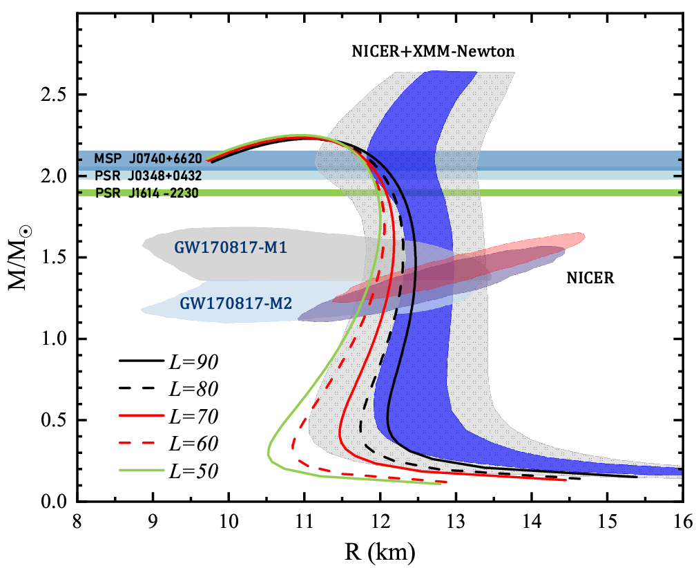
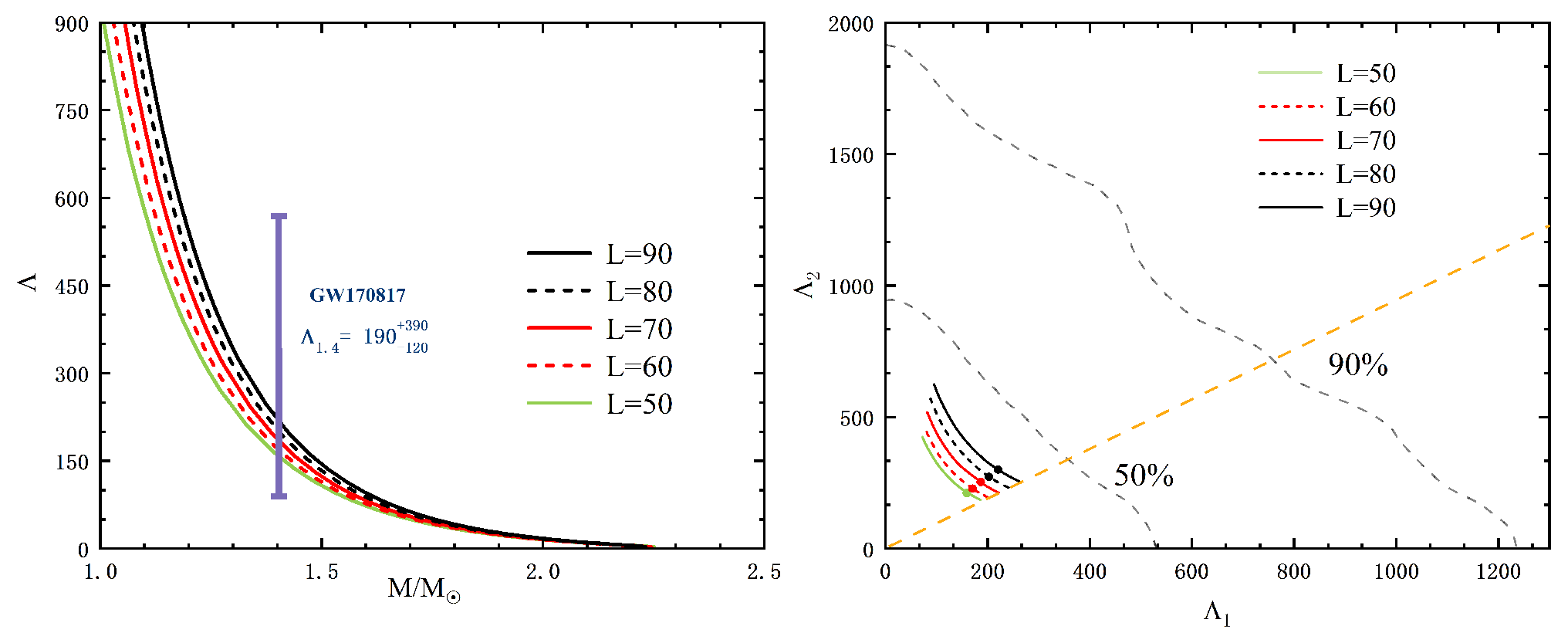
As a whole, after taking into account the SRC and admixed DM in NS interior, the five parameter sets constructed by varying based on the GM1 can not only characterize the behavior of nuclear matter at low densities (Figs.2-4), but also meet the requirements inferred from recent multi-messenger observations (Figs.5-6). Next, using these parameter sets, we investigate the effect of on the currently undetectable NS oscillation frequencies.
IV Non-radial oscillation and radial oscillation
IV.1 Non-radial oscillation
Thorne and Campollataro (Thorne and Campolattaro 1967) are credited with being the ones who first suggested discussing non-radial modes within the context of general relativity. In our work, we consider a non-rotating NS with an ideal fluid interior, using the Cowling approximation (Cowling 1941; McDermott et al. 1983; Torres-Forné et al. 2017), which ignores the space-time metric perturbation but retains density perturbations caused by fluid oscillations (Kokkotas and Schmidt 1999). Recent research indicates that the difference between the -mode calculated using the Cowling approximation approach and the complete linearized equations of general relativity is less than 20%, the -mode error is about 10% (Yoshida and Kojima 1997), and the -mode error is only a few percent (Sotani et al. 2001). This shows the practicality of Cowling approximation (Flores and Lugones 2014), and based on this, the fluid perturbations consist of a spherical harmonic function and a time-dependent part eiωt, resulting in the following Lagrangian fluid displacements associated with infinitesimal oscillatory perturbations:
| (19) | |||||
where and satisfy
| (20) | |||
with
| (21) |
the above equations can be viewed as the eigenvalue equations of for suitable boundary conditions. Inside NS(), and exhibit the following approximate behaviors:
| (22) |
with A being an arbitrary constant. The outer boundary condition is the pressure will disappear at the NS surface
| (23) |
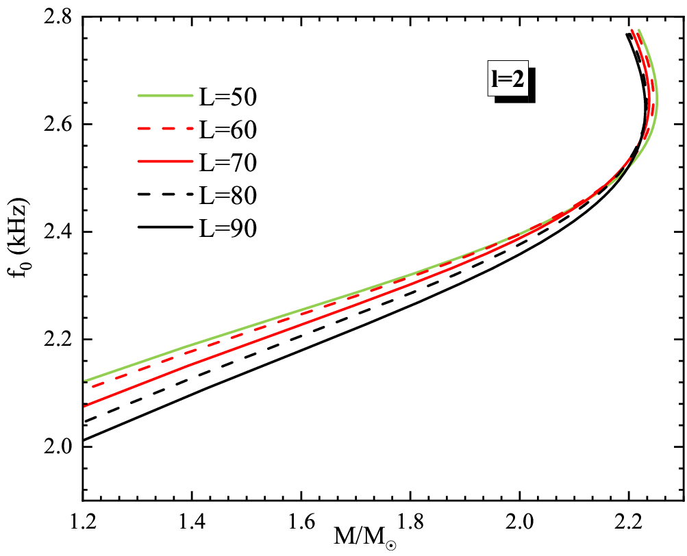
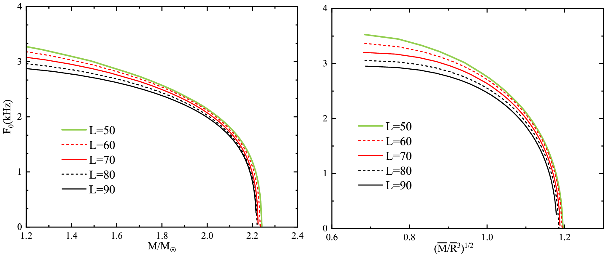
In this paper, we determine the typical non-radial bar mode instability for quadrupole oscillations ( = 2) (Passamonti et al. 2013) using the above revised parameter sets, and show the -mode frequencies under different s in Fig.7. If we take a closer look at the region roughly between and , a smaller is more likely to excite -mode oscillations, giving a larger frequency. The curve starts to bend after approaching maximum mass, after which it corresponds to the unstable NS. In the stable region, the frequency increases with mass, for , different s give frequencies in the range of 2.10 kHz-2.19 kHz, and for , in the range of 2.35 kHz-2.39 kHz. If future gravitational wave detectors like the Cosmic Explorer or Einstein Telescope (Perkins et al. 2021; Punturo et al. 2010; Dwyer et al. 2015) are able to pick up the frequency in this range, we may have a good reason to speculate about the approximate mass of this NS.
In GW asteroseismology, we can relate the oscillation frequency and damping timescale to NS bulk properties like mass, radius, and tidal deformability, and then establish an empirical relationship between them (Doneva et al. 2013; Benhar et al. 2004; Passamonti et al. 2013; Gaertig et al. 2011; Pradhan and Chatterjee 2021; Wen et al. 2019). The original study was proposed by Andersson and Kokkotas (Andersson and Kokkotas 1996; Andersson and Kokkotas 1998), who suggested that the stellar dynamical timescale is related to its mean density and established a empirical relationship as
| (24) |
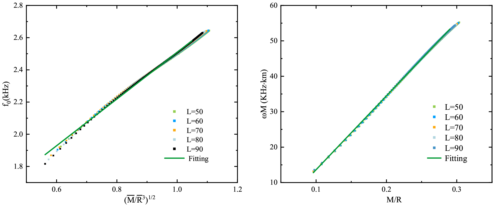
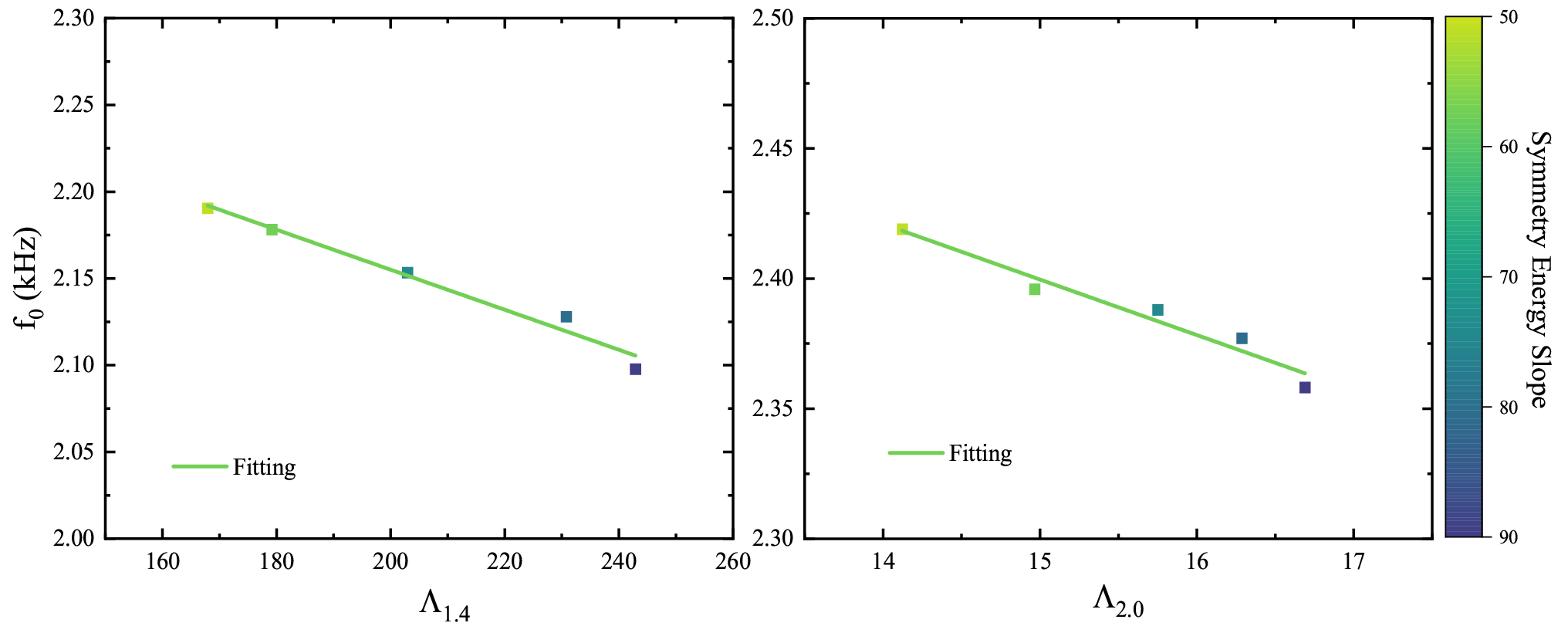
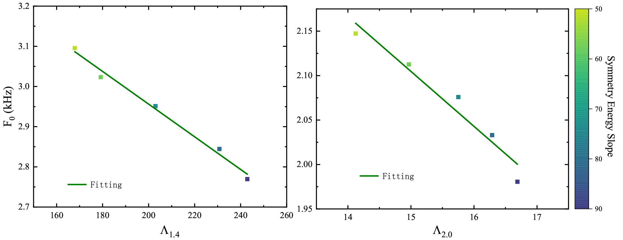
where the dimensionless parameters and . A further evaluation of this relationship was carried out by taking into account the rotation effect (Doneva et al. 2013) and exotic matter (Benhar et al. 2004) in the NS. However, these studies are not supported by the current results of multi-messenger astronomy and need further adjustment. Our goal is to re-calibrate this empirical relationship by considering SRC and admixed DM inside NSs, with satisfying the behaviours near saturation density and multi-messenger observations. The specific results are shown on the left in Fig.8, where the different scatter points indicate the results given by different s and the solid green line is the result of linear fitting. We present the fitting result in Table 2, as a comparison, we also present the results by other researchers. It is found that incorporating SRC and DM within NSs still maintains a good linear relationship, and the discrepancies are very small compared to other models, further illustrating the model-independent nature. Another similar scenario is that of a excellent linear correlation between and , which has been used to analyze -mode, -mode, and -mode, and the fitting is shown in the right of Fig.8 with , which shows a stronger linear correlation than the case on the left. These empirical relations can be used to easily decode NS internal information once the -mode frequencies can be detected. On the one hand, the -mode frequency is capable of not only providing information on the NS density, but also inferring the compactness () which further correlates to NS tidal deformability. On the other hand, as the NICER detector are upgraded to simultaneously give accurate masses and radii in the foreseeable future, we can in turn be able to predict its -mode frequency well. As mentioned, since the compactness controls the tidal deformability directly, we can also relate the -mode frequency to the tidal deformability by extrapolating the relationship between -mode and compactness. For this purpose we plot and with the corresponding -mode frequencies in Fig.9, where the dots in different shades indicate different s. It can be found that the larger is, the larger corresponding radius is (see Fig.5 for details), and the NS is more likely to undergo a deformation resulting in a larger tidal deformability (see Fig.6), but a larger radius is more conducive to NS stability and thus more difficult to vibrate(see Fig.7), so the larger , the larger tidal deformability and the smaller -mode frequency. Furthermore, the frequency and tidal deformability show a good linear correlation, and we have fitted with and , and the range of and extracted from different both satisfy the constraints from GW170817 and theoretical calculations (De et al. 2018). This connection not only explains the influence of on frequency and tidal deformability, but it also predicts the observations. Together with the empirical relation shown in Fig.8, the constraints on the EOSs will become increasingly rigorous.
| CASES | a(kHz) | b(kHz) | |
|---|---|---|---|
| SRC and admixed DM | 1.0581 | 1.4507 | |
| Andersson and Kokkotas | 0.78 | 1.6350 | |
| (Andersson and Kokkotas 1996) | |||
| Omar Benhar et al. | 0.79 | 1.5000 | |
| (Benhar et al. 2004) | |||
| Daniela D. Doneva et al. | 1.5620 | 1.1510 | |
| (Doneva et al. 2013) | |||
| Bikram Keshari Pradhan et al. | 1.0750 | 1.4120 | |
| (Pradhan and Chatterjee 2021) |
IV.2 Radial oscillation
It has been shown that radial oscillations of NSs, accompanied by non-radial oscillations(Passamonti et al. 2007), are a special class of non-radial oscillations, which in astroseismology correspond to spherical harmonic functions with zero orbital angular momentum. A seminal paper by Chandrasekhar (Chandrasekhar 1964) was the first to discuss radial perturbations of compact stars and in the past 60 years, different work has been done to study the NSs’ radial oscillations under the general relativity (Glass and Lindblom 1983; Chanmugam 1977; Passamonti et al. 2006; Passamonti et al. 2007; Di Clemente et al. 2020; Sagun et al. 2020; Sun et al. 2021). Some studies have pointed out that radial oscillation can be used to distinguish between traditional NSs and strange stars (Vaeth and Chanmugam 1992) as well as hybrid stars (Pereira et al. 2018; Sun et al. 2021), and can also often be used to describe the NS stability. Despite the fact that radial oscillations cannot directly produce gravitational radiation, they can couple and amplify gravitational wave signals (Passamonti et al. 2006; Passamonti et al. 2007). As described in Ref.(Gondek et al. 1997), the differential equations that characterize infinitesimal radial oscillations can be expressed as:
| (25) |
| (26) | |||||
where is the radial eigenfrequency, () and characterize the radial displacement and Lagrangian perturbation of pressure respectively, both of which rely on the harmonic time form of . stands for the relativistic adiabatic index:
| (27) |
Numerically solving above equations requires two boundary conditions, one is that in the NS interior ( = 0) the term associated with must be finite (Gondek et al. 1997), so we have
| (28) |
with for the normalization condition and the second one is that the pressure perturbation near NS surface should become negligible, i.e. for . Taking a given NS EOS as an input, the above oscillation equations are Sturm-Liouville boundary value problems (Vaeth and Chanmugam 1992) and using the numerical shooting method we can get a series of so-called eigenvalue frequencies , with being the number of nodes.
| Overtone number | =50 MeV | =60 MeV | =70 MeV | =80 MeV | =90 MeV | |||||
|---|---|---|---|---|---|---|---|---|---|---|
| =1 | 3.095 (2.142) | 3.031 (2.113) | 2.952 (2.074) | 2.861 (2.031) | 2.777 (1.991) | |||||
| =2 | 7.885 (7.086) | 7.705 (7.031) | 7.498 (6.952) | 7.284 (6.842) | 7.090 (6.735) | |||||
| =3 | 12.141 (11.129) | 11.839 (11.029) | 11.507 (10.895) | 11.183 (10.715) | 10.888 (10.545) | |||||
| =4 | 16.288 (15.025) | 15.871 (14.877) | 15.417 (14.687) | 14.991 (14.441) | 14.594 (14.213) | |||||
| =5 | 20.395 (18.868) | 19.866 (18.671) | 19.294 (18.425) | 18.765 (18.114) | 18.256 (17.824) | |||||
| =6 | 24.482 (22.683) | 23.844 (22.438) | 23.153 (22.137) | 22.522 (21.768) | 21.906 (21.415) | |||||
| =7 | 28.558 (26.484) | 27.814 (26.192) | 26.999 (25.835) | 26.261 (25.401) | 25.516 (24.994) | |||||
| =8 | 32.626 (30.275) | 31.777 (29.936) | 30.829 (29.526) | 29.978 (29.031) | 29.066 (28.565) | |||||
| =9 | 36.688 (34.061) | 35.734 (33.676) | 34.638 (33.212) | 33.661 (32.657) | 32.521 (32.131) | |||||
| =10 | 40.746 (37.842) | 39.684 (37.412) | 38.417 (36.894) | 37.392 (36.280) | 35.815 (35.694) | |||||
| =11 | 44.798 (41.620) | 43.628 (41.145) | 42.158 (40.575) | 40.872 (39.901) | 38.895 (39.253) |
Our next step is to examine how influences radial oscillations in terms of fundamental radial frequencies () and consecutive frequency differences (so-called Large Separation) (Lopes, I. P. 2001; Panotopoulos and Lopes 2017b). The fundamental radial frequencies () as a function of NS mass are given on the left of Fig.10. The smaller exhibit larger radial frequency, similar to the result from non-radial one, and the effect of on the frequency is more pronounced in low mass regions, where the frequency drops from 3.11 kHz ( MeV) to 2.76 kHz ( MeV) for 1.4 and from 2.16 kHz to 1.99 kHz for 2. Furthermore, unlike non-radial oscillations, the radial frequency decreases more rapidly at massive NS regions, and tends to zero when the mass indefinitely approaches the maximum stable mass (MSM). This is because when a NS reaches its MSM, any small radial perturbation does not cause the star to oscillate. Due to this fact, the linear relationship between the radial frequency and the mean density is no longer satisfied as it was for the non-radial one (see the right of Fig.10). Moreover, we can apply radial frequency equivalently to determine the star equilibrium condition, where a stable NS condition requires in the mass-radius curve, in which gives the MSM, corresponding to the point in figure where the frequency is zero. This is important because the MSM obtained from the mass-radius curve can only be given by a theoretical model calculation, whereas the radial oscillation frequency allows the MSM to be determined from an observed perspective. Combined with the results from non-radial oscillations together, we can infer whether the NS has a MSM, as radial oscillations are less likely to occur near the MSM (see Fig.10), while non-radial oscillations are more likely to produce high frequencies (see Fig.7), which means that if a small radial frequency be detected along with a high non-radial frequency, the NS is closer to its MSM. This will be possible in the near future with the upgrade of high-sensitivity GW detectors, and from this point of view, NS astroseismology could provide at least one new way to determine the NS MSM.
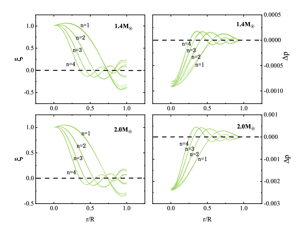
For high-mode oscillations with overtone numbers , we examined the implications of for their eigenfunctions. Fig.11 shows the first four high-mode eigenfunctions, with shown in the left part and in the right, and 1.4 and 2 correspond to upper and down panel, respectively. The intersection of eigenfunction curve with dash-line represents the overtone number, for example, =1 indicates that there is only one node. Furthermore, as the overtone numbers increase, the curve fluctuations become more prominent and reflect a higher frequency. In the NS interior, the different symmetry energy slopes (corresponding to different lines under each overtone curve) have little impact on the high-mode oscillation. It is essential to emphasize that the -mode still remains the most promising frequency band for detection since the larger overtone numbers produce higher the frequencies, which would far exceed the sensitivity of current detection devices, making it still difficult to detect.
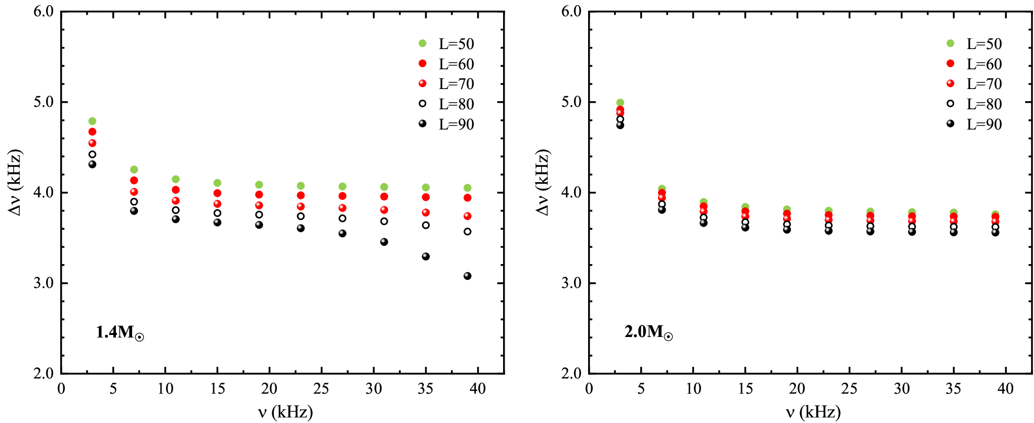
The consecutive frequency differences or Large Separation (LS) can also be extracted from the high-mode eigenfunctions, which is a measurable quantity that has been used to identify the DM component(Panotopoulos and Lopes 2017b). To further examine the possible implications from , we calculated 11 consecutive high-mode oscillation frequencies listed in Table 3, and plot the results in Fig.12, with the left and right parts showing 1.4 and 2 cases, respectively. It can be seen that the LS in both cases is roughly around 4 kHz to 5 kHz, which is consistent with the study of strange quark stars admixed DM (Panotopoulos and Lopes 2017b). Moreover, LS decreases as increases, where for 1.4 the decrease in LG is about 0.8 kHz or more as grows from 50 MeV to 90 MeV, while for 2 LG decreases by approximately 0.4 kHz, which implies that the effect of on LG is more pronounced for low-mass NS than for massive NS, as also implied from the previous discussion on this point (see Figs.5-6). Finally, as discussed in section 4.1, the non-radial oscillations give a very strong linear correlation between frequency and tidal deformability for different s, and as an analogy we also give results for the radial ones, apart from the different frequency values, 1.4 and 2 also satisfy a fairly good linear relationship, with the fitted results being and shown in Fig.13 respectively. These results together with the non-radial oscillations will be more helpful in constraining EOSs for NSs.
V Summary
In this study, we absorb the nucleon-nucleon SRC and admixed DM effect in NS interior, adopting the widely accepted SRC model and assuming the DM component to be one thousandth of the conventional nucleon number density. As a result of incorporating SRC and DM, we re-derive the pressure and energy density at the relativistic mean field theory and revise the corresponding nucleon coupling parameters. It is found that the simultaneous introduction of SRC and DM enables NS to better satisfy the observational constraints, and on this basis a typical set of parameters GM1 is selected to evaluate the impact of on the oscillation frequency of NSs with incorporating SRC and DM. For the purpose of verifying the feasibility of sets constructed from different s, we calculated its behavior at low and high densities and discovered that it not only fulfills the properties near the saturation nuclear matter density well, but also meets the astronomical constraints. The following are the important physical findings of this study.
1. For non-radial oscillations, absorbing SRC and DM, the smaller is more likely to excite -mode for stable NSs, thus giving larger frequencies.
2. After absorbing SRC and DM, we updated the empirical relationship between frequency and mean density with , and the relationship between and the compactness parameter with , these relations can be used to decode NS internal information from the -mode frequencies.
3. Our results indicate that a larger results in a larger tidal deformability and a smaller non-radial frequency. Furthermore, the frequency and tidal deformability show a good linear correlation, corresponding to and for 1.4 and 2.
4. For fundamental radial oscillations, the smaller exhibit larger radial frequency, and the effect of on the frequency is more pronounced in low mass regions, where the frequency drops from 3.11 kHz to 2.76 kHz for 1.4 and from 2.16 kHz to 1.99 kHz for 2 as changes from 50 MeV to 90 MeV. Moreover, with the features of non-radial frequencies, we can provide a methodology for estimating the maximum stable mass of NS.
5. Finally, we evaluate the effect of on the high-mode eigenfunction as well as LG, and find that the has little impact on the high-mode oscillation and the effect on LG is more pronounced for low-mass NS than for massive NS. We also found that the frequency of radial oscillations also satisfies a strong linear relationship with tidal deformability, for which we fitted this relationship at 1.4 and 2, corresponding to and , respectively.
The above findings establish a link between and NS oscillation frequency, which allows us to understand how the affects the frequency and on other NS properties, with the continuous improvement of observational equipments, it is anticipated that this band frequency will be observed in the future, which in turn can be used to constrain .
Acknowledgements.
Bin thanks the anonymous referee for his or her kind guidance. This work is supported by the National Natural Science Foundation of China ( Grants No.12035011, No.11975167, No.11961141003, No.11905103, No.11761161001, No.11375086), and by the National Key R&D Program of China (Contracts No. 2018YFA0404403 and No.2016YFE0129300).Data Availability Statement
This manuscript has no associated data or the data will not be deposited. [Authors’ comment: All results are shown in figures or table and are clearly given. The experimental data we cited can be obtained from references.]
appendix
In this study within SRC-revised RMFT, in addition to the energy density and pressure that need to be revised, the six nucleon coupling parameters of also need to be revised, which rely on the saturation number density , binding energy per nucleon , incompressibility coefficient and nucleon effective mass . Next we will re-derive their connection by considering SRC effect. Given that the sum of binding energy per nucleon and nucleon mass determine energy per nucleon , i.e. , thus we can yield
| (29) |
where stands for the nucleon effective mass, and since the isospin-asymmetry for saturation density, we get , , . As described in RMFT, the isoscalar-scalar meson meet
| (30) |
and energy density satisfies as
| (31) |
At saturation density, the incompressibility coefficient reads as
where prime refers to the partial derivative of momentum and nucleon effective mass , and ,, and read as
| (33) | |||||
| (34) | |||||
| (35) | |||||
Moreover, we can correlate the isovector coupling parameters and with symmetry energy and its slope , for symmetry energy at saturation density, it can be divided into two parts and reads as
| (37) |
where two parts correspond to
| (38) |
and
| (39) |
While, for symmetry energy slope , it also can be divided into two parts accordingly
| (40) |
where represent as
| (41) |
and
At this point, it is clear that the six nucleon coupling parameters under the SRC-revised RMFT are successfully associated with six saturation nuclear parameters, and can be quantitatively solved.
References
- Oertel et al. (2017) M. Oertel, M. Hempel, T. Klähn, and S. Typel, Rev. Mod. Phys. 89, 015007 (2017).
- Jiang et al. (2020) J.-L. Jiang, S.-P. Tang, Y.-Z. Wang, et al., The Astrophysical Journal 892, 55 (2020).
- Luo et al. (2022) C.-N. Luo, S.-P. Tang, J.-L. Jiang, W.-H. Gao, and D.-M. Wei, The Astrophysical Journal 930, 4 (2022).
- Epelbaum et al. (2009) E. Epelbaum, H.-W. Hammer, and U.-G. Meißner, Rev. Mod. Phys. 81, 1773 (2009).
- Hammer et al. (2013) H.-W. Hammer, A. Nogga, and A. Schwenk, Rev. Mod. Phys. 85, 197 (2013).
- Holt et al. (2013) J. W. Holt, N. Kaiser, and W. Weise, Progress in Particle and Nuclear Physics 73, 35 (2013).
- Tews et al. (2013) I. Tews, T. Krüger, K. Hebeler, and A. Schwenk, Phys. Rev. Lett. 110, 032504 (2013).
- Lynn et al. (2016) J. E. Lynn, I. Tews, J. Carlson, S. Gandolfi, A. Gezerlis, K. E. Schmidt, and A. Schwenk, Phys. Rev. Lett. 116, 062501 (2016).
- Stone and Reinhard (2007) J. Stone and P.-G. Reinhard, Progress in Particle and Nuclear Physics 58, 587 (2007).
- Rikovska Stone et al. (2003) J. Rikovska Stone, J. C. Miller, R. Koncewicz, P. D. Stevenson, and M. R. Strayer, Phys. Rev. C 68, 034324 (2003).
- Dutra et al. (2012) M. Dutra, O. Lourenço, J. S. Sá Martins, A. Delfino, J. R. Stone, and P. D. Stevenson, Phys. Rev. C 85, 035201 (2012).
- Loan et al. (2011) D. T. Loan, N. H. Tan, D. T. Khoa, and J. Margueron, Phys. Rev. C 83, 065809 (2011).
- Gonzalez-Boquera et al. (2017) C. Gonzalez-Boquera, M. Centelles, X. Viñas, and A. Rios, Phys. Rev. C 96, 065806 (2017).
- Read et al. (2009) J. S. Read, B. D. Lackey, B. J. Owen, and J. L. Friedman, Phys. Rev. D 79, 124032 (2009).
- Demorest et al. (2010) P. B. Demorest, T. Pennucci, S. M. Ransom, et al., Nature 467, 1081 (2010).
- Fonseca et al. (2016) E. Fonseca, T. T. Pennucci, J. A. Ellis, et al., The Astrophysical Journal 832, 167 (2016).
- Arzoumanian et al. (2018) Z. Arzoumanian, A. Brazier, S. Burke-Spolaor, et al., The Astrophysical Journal Supplement Series 235, 37 (2018).
- Antoniadis et al. (2013) J. Antoniadis, P. C. C. Freire, N. Wex, et al., Science 340 (2013).
- Cromartie et al. (2020) H. T. Cromartie, E. Fonseca, S. M. Ransom, et al., Nature Astronomy 4, 72 (2020).
- Fonseca et al. (2021) E. Fonseca, H. T. Cromartie, and T. T. Pennucci, The Astrophysical Journal Letters 915, L12 (2021).
- Abbott et al. (2019) B. P. Abbott, R. Abbott, T. D. Abbott, et al. (LIGO Scientific Collaboration and Virgo Collaboration), Phys. Rev. X 9, 011001 (2019).
- Fasano et al. (2019) M. Fasano, T. Abdelsalhin, A. Maselli, and V. Ferrari, Phys. Rev. Lett. 123, 141101 (2019).
- Miller et al. (2019) M. C. Miller, F. K. Lamb, A. J. Dittmann, et al., The Astrophysical Journal 887, L24 (2019).
- Riley et al. (2019) T. E. Riley, A. L. Watts, S. Bogdanov, et al., The Astrophysical Journal 887, L21 (2019).
- Abbott et al. (2020) R. Abbott, T. D. Abbott, S. Abraham, et al., The Astrophysical Journal 896, L44 (2020).
- Arrington et al. (2012) J. Arrington, D. Higinbotham, G. Rosner, and M. Sargsian, Progress in Particle and Nuclear Physics 67, 898 (2012).
- degli Atti (2015) C. C. degli Atti, Physics Reports 590, 1 (2015).
- Hen et al. (2017) O. Hen, G. A. Miller, E. Piasetzky, and L. B. Weinstein, Rev. Mod. Phys. 89, 045002 (2017).
- Rohe et al. (2004) D. Rohe, C. S. Armstrong, R. Asaturyan, O. K. Baker, S. Bueltmann, et al. (E97-006 Collaboration), Phys. Rev. Lett. 93, 182501 (2004).
- Onderwater et al. (1998) C. J. G. Onderwater, K. Allaart, E. C. Aschenauer, et al., Phys. Rev. Lett. 81, 2213 (1998).
- Starink et al. (2000) R. Starink, M. Van Batenburg, E. Cisbani, W. Dickhoff, S. Frullani, et al., Physics Letters B 474, 33 (2000).
- Panda et al. (2006) P. K. Panda, J. a. d. Providência, and C. m. c. Providência, Phys. Rev. C 73, 035805 (2006).
- Sammarruca (2014) F. Sammarruca, Phys. Rev. C 90, 064312 (2014).
- Cai and Li (2015) B.-J. Cai and B.-A. Li, Phys. Rev. C 92, 011601 (2015).
- Hen et al. (2015a) O. Hen, B.-A. Li, W.-J. Guo, L. B. Weinstein, and E. Piasetzky, Phys. Rev. C 91, 025803 (2015a).
- Wang et al. (2017) Z. Wang, C. Xu, Z. Ren, and C. Gao, Phys. Rev. C 96, 054603 (2017).
- Yang et al. (2019) Z. X. Yang, X. L. Shang, G. C. Yong, W. Zuo, and Y. Gao, Phys. Rev. C 100, 054325 (2019).
- Weinstein et al. (2011) L. B. Weinstein, E. Piasetzky, D. W. Higinbotham, J. Gomez, O. Hen, and R. Shneor, Phys. Rev. Lett. 106, 052301 (2011).
- Hen et al. (2012) O. Hen, E. Piasetzky, and L. B. Weinstein, Phys. Rev. C 85, 047301 (2012).
- Fields et al. (2013) L. Fields, J. Chvojka, L. Aliaga, et al. (MINERvA Collaboration), Phys. Rev. Lett. 111, 022501 (2013).
- Fiorentini et al. (2013) G. A. Fiorentini, D. W. Schmitz, P. A. Rodrigues, and et al. (MINERvA Collaboration), Phys. Rev. Lett. 111, 022502 (2013).
- Souza et al. (2020a) L. A. Souza, M. Dutra, C. H. Lenzi, and O. Lourenço, Phys. Rev. C 101, 065202 (2020a).
- Hong et al. (2022) B. Hong, Z. Ren, and X.-L. Mu, Chinese Physics C 46, 065104 (2022).
- Li et al. (2019) Z. Li, Z. Ren, B. Hong, H. Lu, and D. Bai, Nuclear Physics A 990, 118 (2019).
- Lu et al. (2021) H. Lu, Z. Ren, and D. Bai, Nuclear Physics A 1011, 122200 (2021).
- Lourenço et al. (2022) O. Lourenço, T. Frederico, and M. Dutra, Phys. Rev. D 105, 023008 (2022).
- Souza et al. (2020b) L. A. Souza, R. Negreiros, M. Dutra, D. P. Menezes, and O. Lourenço, arXiv (2020b).
- Bertone et al. (2005) G. Bertone, D. Hooper, and J. Silk, Physics Reports 405, 279 (2005).
- Bertone and Hooper (2018) G. Bertone and D. Hooper, Rev. Mod. Phys. 90, 045002 (2018).
- Buen-Abad et al. (2022) M. A. Buen-Abad, R. Essig, D. McKeen, and Y.-M. Zhong, Physics Reports 961, 1 (2022).
- Kouvaris and Tinyakov (2011) C. Kouvaris and P. Tinyakov, Phys. Rev. D 83, 083512 (2011).
- Quddus et al. (2020) A. Quddus, G. Panotopoulos, B. Kumar, S. Ahmad, and S. K. Patra, Journal of Physics G: Nuclear and Particle Physics 47, 095202 (2020).
- Das et al. (2021) H. C. Das, A. Kumar, and S. K. Patra, Phys. Rev. D 104, 063028 (2021).
- Das et al. (2020) H. C. Das, A. Kumar, B. Kumar, S. K. Biswal, T. Nakatsukasa, A. Li, and S. K. Patra, Monthly Notices of the Royal Astronomical Society 495, 4893 (2020).
- Kong et al. (2017) H.-Y. Kong, J. Xu, L.-W. Chen, B.-A. Li, and Y.-G. Ma, Phys. Rev. C 95, 034324 (2017).
- Tang et al. (2021) S.-P. Tang, J.-L. Jiang, M.-Z. Han, Y.-Z. Fan, and D.-M. Wei, Phys. Rev. D 104, 063032 (2021).
- Adhikari et al. (2021) D. Adhikari, H. Albataineh, D. Androic, and K. Aniol (PREX Collaboration), Phys. Rev. Lett. 126, 172502 (2021).
- Reed et al. (2021) B. T. Reed, F. J. Fattoyev, C. J. Horowitz, and J. Piekarewicz, Phys. Rev. Lett. 126, 172503 (2021).
- Jones (2002) D. I. Jones, Classical and Quantum Gravity 19, 1255 (2002).
- Kokkotas and Schutz (1992) K. D. Kokkotas and B. F. Schutz, Monthly Notices of the Royal Astronomical Society 255, 119 (1992).
- Lau et al. (2010) H. K. Lau, P. T. Leung, and L. M. Lin, The Astrophysical Journal 714, 1234 (2010).
- Kokkotas and Schmidt (1999) K. D. Kokkotas and B. G. Schmidt, Living Reviews in Relativity 2, 2 (1999).
- Passamonti et al. (2007) A. Passamonti, N. Stergioulas, and A. Nagar, Phys. Rev. D 75, 084038 (2007).
- Passamonti et al. (2006) A. Passamonti, M. Bruni, L. Gualtieri, A. Nagar, and C. F. Sopuerta, Phys. Rev. D 73, 084010 (2006).
- Vaeth and Chanmugam (1992) H. M. Vaeth and G. Chanmugam, A&A 260, 250 (1992).
- Vásquez Flores and Lugones (2010) C. Vásquez Flores and G. Lugones, Phys. Rev. D 82, 063006 (2010).
- Flores et al. (2017) C. V. Flores, Z. B. Hall, and P. Jaikumar, Phys. Rev. C 96, 065803 (2017).
- Ranea-Sandoval et al. (2018) I. F. Ranea-Sandoval, O. M. Guilera, M. Mariani, and M. G. Orsaria, Journal of Cosmology and Astroparticle Physics 2018, 031 (2018).
- Pereira et al. (2018) J. P. Pereira, C. V. Flores, and G. Lugones, The Astrophysical Journal 860, 12 (2018).
- Sun et al. (2021) T.-T. Sun, Z.-Y. Zheng, H. Chen, G. F. Burgio, and H.-J. Schulze, Phys. Rev. D 103, 103003 (2021).
- Jaikumar et al. (2021) P. Jaikumar, A. Semposki, M. Prakash, and C. Constantinou, Phys. Rev. D 103, 123009 (2021).
- Lau and Yagi (2021) S. Y. Lau and K. Yagi, Phys. Rev. D 103, 063015 (2021).
- Bauswein et al. (2014) A. Bauswein, N. Stergioulas, and H.-T. Janka, Phys. Rev. D 90, 023002 (2014).
- Takami et al. (2014) K. Takami, L. Rezzolla, and L. Baiotti, Phys. Rev. Lett. 113, 091104 (2014).
- Sotani et al. (2012a) H. Sotani, K. Nakazato, K. Iida, and K. Oyamatsu, Phys. Rev. Lett. 108, 201101 (2012a).
- Sotani et al. (2012b) H. Sotani, K. Nakazato, K. Iida, and K. Oyamatsu, Monthly Notices of the Royal Astronomical Society: Letters 428, L21 (2012b).
- Sotani et al. (2018) H. Sotani, K. Iida, and K. Oyamatsu, Monthly Notices of the Royal Astronomical Society 479, 4735 (2018).
- Sotani et al. (2019) H. Sotani, K. Iida, and K. Oyamatsu, Monthly Notices of the Royal Astronomical Society 489, 3022 (2019).
- Perkins et al. (2021) S. E. Perkins, N. Yunes, and E. Berti, Phys. Rev. D 103, 044024 (2021).
- Punturo et al. (2010) M. Punturo, M. Abernathy, F. Acernese, and et al., Classical and Quantum Gravity 27, 084007 (2010).
- Dwyer et al. (2015) S. Dwyer, D. Sigg, S. W. Ballmer, L. Barsotti, N. Mavalvala, and M. Evans, Phys. Rev. D 91, 082001 (2015).
- Panotopoulos and Lopes (2017a) G. Panotopoulos and I. Lopes, Phys. Rev. D 96, 083004 (2017a).
- Murakami and Wells (2001) B. Murakami and J. D. Wells, Phys. Rev. D 64, 015001 (2001).
- Cline et al. (2013) J. M. Cline, P. Scott, K. Kainulainen, and C. Weniger, Phys. Rev. D 88, 055025 (2013).
- Tan et al. (2016) A. Tan et al. (PandaX-II Collaboration), Phys. Rev. Lett. 117, 121303 (2016).
- Meng et al. (2021) Y. Meng et al. (PandaX-4T Collaboration), Phys. Rev. Lett. 127, 261802 (2021).
- Dickhoff and Van Neck (2008) W. H. Dickhoff and D. Van Neck, Many-Body Theory Exposed!, 2nd ed. (WORLD SCIENTIFIC, 2008).
- Rios et al. (2014) A. Rios, A. Polls, and W. H. Dickhoff, Phys. Rev. C 89, 044303 (2014).
- Rios (2020) A. Rios, Journal of Physics: Conference Series 1643, 012164 (2020).
- Guo et al. (2021) W.-M. Guo, B.-A. Li, and G.-C. Yong, Phys. Rev. C 104, 034603 (2021).
- Subedi et al. (2008) R. Subedi, R. Shneor, P. Monaghan, B. D. Anderson, K. Aniol, J. Annand, J. Arrington, H. Benaoum, F. Benmokhtar, W. Boeglin, and J.-P. Chen, Science 320, 1476 (2008).
- Hen et al. (2015b) O. Hen, L. B. Weinstein, E. Piasetzky, G. A. Miller, M. M. Sargsian, and Y. Sagi, Phys. Rev. C 92, 045205 (2015b).
- Baym et al. (1971) G. Baym, C. Pethick, and P. Sutherland, Astrophys. J. 170, 299 (1971).
- Cai and Li (2016) B.-J. Cai and B.-A. Li, Phys. Rev. C 93, 014619 (2016).
- Xu et al. (2009) J. Xu, L.-W. Chen, B.-A. Li, and H.-R. Ma, Phys. Rev. C 79, 035802 (2009).
- Carriere et al. (2003) J. Carriere, C. J. Horowitz, and J. Piekarewicz, The Astrophysical Journal 593, 463 (2003).
- Oppenheimer and Volkoff (1939) J. Oppenheimer and G. Volkoff, Physical Review 55, 374 (1939), cited By 1756.
- Lalazissis et al. (1997) G. A. Lalazissis, J. König, and P. Ring, Phys. Rev. C 55, 540 (1997).
- Todd-Rutel and Piekarewicz (2005) B. G. Todd-Rutel and J. Piekarewicz, Phys. Rev. Lett. 95, 122501 (2005).
- Glendenning and Moszkowski (1991) N. K. Glendenning and S. A. Moszkowski, Phys. Rev. Lett. 67, 2414 (1991).
- Liu et al. (2002) B. Liu, V. Greco, V. Baran, M. Colonna, and M. Di Toro, Phys. Rev. C 65, 045201 (2002).
- Abbott et al. (2017) B. P. Abbott, R. Abbott, T. D. Abbott, et al. (LIGO Scientific Collaboration and Virgo Collaboration), Phys. Rev. Lett. 119, 161101 (2017).
- Abbott et al. (2018) B. P. Abbott, R. Abbott, T. D. Abbott, et al. (The LIGO Scientific Collaboration and the Virgo Collaboration), Phys. Rev. Lett. 121, 161101 (2018).
- Annala et al. (2018) E. Annala, T. Gorda, A. Kurkela, and A. Vuorinen, Phys. Rev. Lett. 120, 172703 (2018).
- Most et al. (2018) E. R. Most, L. R. Weih, L. Rezzolla, and J. Schaffner-Bielich, Phys. Rev. Lett. 120, 261103 (2018).
- De et al. (2018) S. De, D. Finstad, J. M. Lattimer, D. A. Brown, E. Berger, and C. M. Biwer, Phys. Rev. Lett. 121, 091102 (2018).
- Miller et al. (2021) M. C. Miller, F. K. Lamb, A. J. Dittmann, et al., The Astrophysical Journal Letters 918, L28 (2021).
- Riley et al. (2021) T. E. Riley et al., The Astrophysical Journal Letters 918, L27 (2021).
- Hornick et al. (2018) N. Hornick, L. Tolos, A. Zacchi, J.-E. Christian, and J. Schaffner-Bielich, Phys. Rev. C 98, 065804 (2018).
- Wu et al. (2021) X. Wu, S. Bao, H. Shen, and R. Xu, Phys. Rev. C 104, 015802 (2021).
- Hu et al. (2020) J. Hu, S. Bao, Y. Zhang, K. Nakazato, K. Sumiyoshi, and H. Shen, Progress of Theoretical and Experimental Physics 2020 (2020).
- Huang et al. (2020) K. Huang, J. Hu, Y. Zhang, and H. Shen, The Astrophysical Journal 904, 39 (2020).
- Cavagnoli et al. (2011) R. Cavagnoli, D. P. Menezes, and C. m. c. Providência, Phys. Rev. C 84, 065810 (2011).
- Danielewicz et al. (2002) P. Danielewicz, R. Lacey, and W. G. Lynch, Science 298, 1592 (2002).
- Thorne and Campolattaro (1967) K. S. Thorne and A. Campolattaro, The Astrophysical Journal 149, 591 (1967).
- Cowling (1941) T. G. Cowling, Monthly Notices of the Royal Astronomical Society 101, 367 (1941).
- McDermott et al. (1983) P. N. McDermott, H. M. van Horn, and J. F. Scholl, The Astrophysical Journal 268, 837 (1983).
- Torres-Forné et al. (2017) A. Torres-Forné, P. Cerdá-Durán, A. Passamonti, and J. A. Font, Monthly Notices of the Royal Astronomical Society 474, 5272 (2017).
- Yoshida and Kojima (1997) S. Yoshida and Y. Kojima, Monthly Notices of the Royal Astronomical Society 289, 117 (1997).
- Sotani et al. (2001) H. Sotani, K. Tominaga, and K.-i. Maeda, Phys. Rev. D 65, 024010 (2001).
- Flores and Lugones (2014) C. V. Flores and G. Lugones, Classical and Quantum Gravity 31, 155002 (2014).
- Passamonti et al. (2013) A. Passamonti, E. Gaertig, K. D. Kokkotas, and D. Doneva, Phys. Rev. D 87, 084010 (2013).
- Doneva et al. (2013) D. D. Doneva, E. Gaertig, K. D. Kokkotas, and C. Krüger, Phys. Rev. D 88, 044052 (2013).
- Benhar et al. (2004) O. Benhar, V. Ferrari, and L. Gualtieri, Phys. Rev. D 70, 124015 (2004).
- Gaertig et al. (2011) E. Gaertig, K. Glampedakis, K. D. Kokkotas, and B. Zink, Phys. Rev. Lett. 107, 101102 (2011).
- Pradhan and Chatterjee (2021) B. K. Pradhan and D. Chatterjee, Phys. Rev. C 103, 035810 (2021).
- Wen et al. (2019) D.-H. Wen, B.-A. Li, H.-Y. Chen, and N.-B. Zhang, Phys. Rev. C 99, 045806 (2019).
- Andersson and Kokkotas (1996) N. Andersson and K. D. Kokkotas, Phys. Rev. Lett. 77, 4134 (1996).
- Andersson and Kokkotas (1998) N. Andersson and K. D. Kokkotas, Monthly Notices of the Royal Astronomical Society 299, 1059 (1998).
- Chandrasekhar (1964) S. Chandrasekhar, Phys. Rev. Lett. 12, 114 (1964).
- Glass and Lindblom (1983) E. N. Glass and L. Lindblom, The Astrophysical Journal Letters 53, 93 (1983).
- Chanmugam (1977) G. Chanmugam, The Astrophysical Journal 217, 799 (1977).
- Di Clemente et al. (2020) F. Di Clemente, M. Mannarelli, and F. Tonelli, Phys. Rev. D 101, 103003 (2020).
- Sagun et al. (2020) V. Sagun, G. Panotopoulos, and I. Lopes, Phys. Rev. D 101, 063025 (2020).
- Gondek et al. (1997) D. Gondek, P. Haensel, and J. L. Zdunik, A&A 325, 217 (1997).
- Lopes, I. P. (2001) Lopes, I. P., A&A 373, 916 (2001).
- Panotopoulos and Lopes (2017b) G. Panotopoulos and I. Lopes, Phys. Rev. D 96, 083013 (2017b).