On the Energy-Efficiency Trade-off Between
Active and Passive Communications with
RIS-based Symbiotic Radio

The sixth generation (6G) mobile communication networks are expected to support ultra-broadband transmission, ultra-massive access, ubiquitous sensing, and reliable intelligent connectivity[2, 3, 4]. However, with the dramatic increase of connected communication devices, there are two serious challenges: the shortage of spectrum resources and the sustainability of energy supply. To resolve such issues, it is imperative to develop innovative technologies to simultaneously improve the spectrum efficiency (SE) and energy efficiency (EE) to fully realize the vision of Internet of Everything (IoE).

One promising solution to address the above challenge is symbiotic radio (SR) communication[5], which combines the advantages and effectively avoids the deficiencies of both cognitive radio (CR)[6] and cooperative ambient backscatter communication (AmBC)[7]. The key idea of SR is to leverage cognitive backscattering communication to achieve mutualistic spectrum and energy sharing by integrating passive backscatter device (BD) with active primary transmitter (PT). Specifically, the BD modulates its own information by passively backscattering the incident signal from the PT without active signal processing. As such, apart from enhancing SE as in the conventional CR system, SR exploits the passive backscattering technology to greatly reduce the power consumption as in the AmBC system, which is expected to improve EE significantly[8]. In general, SR can be classified into two categories, parasitic SR (PSR) and commensal SR (CSR), according to the relationships between the symbol periods for the BD and the PT[5]. In PSR, the signals of both BD and PT have equal symbol durations, so that the backscattering transmission and the primary transmission interfere with each other. By contrast, in CSR, the symbol duration of the passive BD signal spans multiple PT symbol durations, which may contribute additional multipath signal components to enhance the active primary transmission[5]. SR communication is expected to find a wide range of applications, such as E-health, wearable devices, environmental monitoring, vehicle-to-everything (V2E), and smart city[9].

Significant research efforts have been recently devoted to the study of SR communications, e.g., in terms of theoretical analysis[10] and performance optimization to maximize the achievable rate[11], channel capacity[12] and EE[13]. However, a practical challenge of SR technique is that due to the double-hop signal attenuations, the backscattering link is typically much weaker than the direct primary link[8]. Thus, the performance of the secondary passive communication and its additional multipath contribution to the primary communication link are quite limited. To address such issues, various techniques have been proposed to enhance the backscattering links, such as massive BDs enabled SR[14, 15, 16] or active-load assisted SR[17] communications. In particular, multiple-input multiple-output (MIMO) SR communication system with massive number of BDs is studied in [15], where closed-form expressions of the asymptotic regime are derived to reveal the relationship between the primary and secondary communication rates. Besides, a precoding optimization problem is solved to maximize the primary communication rate while guaranteeing the minimum secondary communication rate.

On the other hand, reconfigurable intelligent surface (RIS), also termed as intelligent reflecting surface (IRS)[18], has emerged as another promising solution to strengthen the backscattering link. RIS is composed of a large number of passive reflecting elements, which is able to configure the wireless environment in a desirable manner by adjusting the reflection coefficients without relying on active radio frequency (RF) chain components[19, 20]. This prominent property renders RIS rather appealing to enhance the performance of various wireless communication systems, such as CR[21], MIMO[22], unmanned aerial vehicle[23] and non-orthogonal multiple access (NOMA) systems[24]. Unlike such works on RIS-assisted communications, for RIS-based SR systems, the RIS is used not only as a helper to assist the primary active communication, but also as a BD to enable secondary passive communication to transmit its own information[25]. To distinguish it with the conventional counterpart, we term such kind of RIS as RIS-BD in this paper.

Performance optimization for RIS-BD based SR systems has been studied for different purposes, such as power minimization[26, 27, 28] and channel capacity maximization[29]. Specifically, in [26], an algorithm based on generalized power method (GPM) technique is proposed to minimize the transmit power in a RIS empowered SR over broadcasting signals. A RIS-assisted MIMO symbiotic communications adopting multiple reflecting patterns is investigated in [29] to maximize the capacity. Furthermore, novel schemes that incorporate RIS-based SR for symbiotic active/passive communications have also attracted increasing interest. In [30], an optimization framework for the symbiotic operation of a multiuser CR network consisting of a NOMA-based primary network and a RIS-based secondary network is developed. The authors of [31] propose RIS-aided number modulation, where the number of RIS elements are divided into the in-phase and quadrature subsets to transmit the RIS’s information.

However, it is worth noting that there are only very limited works on EE study for RIS-BD based SR communication systems. A RIS-assisted SR communication network with multiple primary users (PUs) and multiple clusters of IoT devices linked with a RIS is considered in [32]. The authors maximize the EE by using alternating optimization (AO) together with semi-definite relaxation (SDR) and Dinkelbach’s algorithm. In [33], the authors propose a method based on the accelerated generalized Benders decomposition (GBD) algorithm to maximize the EE of the secondary receiver under a required signal-to-interference-plus-noise ratio (SINR) constraint for the primary receiver (PR). It is worth remarking that such existing EE studies of RIS-BD based SR systems mainly focus on the so-called global EE, defined as the ratio of the weighted sum-rate of primary and backscattering communications to the total power consumption of passive and active devices. However, considering global EE may lead to the overlook of the EE of RIS-BD since both the communication rate and power consumption of active communication are typically orders of magnitude higher than that of the passive communication. Different from global EE, studying the individual EEs of passive RIS-BD and active PT may reveal the fundamental relationship of EEs between active and passive communications. Therefore, in this paper, we investigate a RIS-BD based multiple-input single-output (MISO) SR communication system. In order to develop an insightful analysis of the EE trade-off between active primary and passive backscattering communications, EE maximization problem is formulated to characterize the EE region. Our main contributions are summarized as follows:

• •

  First, we present the system model of RIS-BD based MISO SR communication systems, and then derive the maximum individual EEs of the active primary communication and the passive backscattering communications. We show that achieving these two maximum EE values require significantly different transmission strategies, which implies that there exist a nontrivial trade-off between these two EEs.

• •

  Next, to exploit the channel hardening effect for RIS-BD based SR systems, we provide the asymptotic analysis by assuming that the number of PT antennas or RIS-BD elements goes very large. We analyze the distribution characteristics of these two EEs in general Rician channel. Besides, closed-form expressions are derived for the EEs of active and passive communications under some special channel assumptions to get some insights.

• •

  Furthermore, to study the fundamental EE trade-off between active and passive communications, we formulate an optimization problem to characterize the Pareto boundary of the EE region. The formulated problem is challenging to be solved, since the variables are coupled and both the objective and the constraints are nonconvex. We propose an effective algorithm termed as sample-average based bisection approach with AO and successive convex approximation (SCA) techniques to transform it into a series of low-complexity convex subproblem. Simulation results are provided to validate our theoretical analysis.

The rest of this paper is organized as follows. Section II presents the system model of RIS-BD based MISO SR communication. Section III derives the maximum individual EEs for the PT and the RIS-BD, respectively. In Section IV, asymptotic performance analysis is provided. In Section V, the Pareto boundary of the EE region is characterized. Simulation results are presented in Section VI. Finally, Section VII concludes this paper.

Notations: Lower- and uppercase letters $x$ and $X$ denote a scalar (or constant) and random variable, respectively. Boldface lower- and uppercase letters $\mathbf{x}$ and $\mathbf{X}$ denote vector and matrix, respectively. Notations $x^{*}$ and $|x|$ denote the conjugate and the absolute value of a scalar, respectively. The L1 norm and L2 norm (also called Euclidean norm) of a vector $\mathbf{x}$ are denoted respectively as $\|\mathbf{x}\|_{1}$ and $\|\mathbf{x}\|$. For a matrix $\mathbf{X}$, denote its conjugate, transpose, and conjugate transpose as ${\mathbf{X}}^{*}$, $\mathbf{X}^{\mathrm{T}}$, and $\mathbf{X}^{\mathrm{H}}$, respectively. $\mathbf{I}_{M}$ denotes an $M\times M$ identity matrix. ${\mathbb{C}^{M\times N}}$ denotes the space of ${M\times N}$ matrices with complex entries. $\mathcal{CN}(\mu,\Sigma)$ denotes the circularly symmetric complex Gaussian (CSCG) distribution with mean $\mu$ and variance $\Sigma$. ${\text{diag}}\left(\mathbf{x}\right)$ denotes a diagonal matrix whose diagonal elements are given by vector $\mathbf{x}$. ${\mathbb{E}_{X}}\left[\cdot\right]$, ${\mathbb{E}[X]}$, $\mathrm{Var}[X]$ and $\mathrm{Cov}[X,Y]$ denote the statistical expectation with respect to $X$, the expectation and variance of $X$, and the covariance between $X$ and $Y$, respectively. Furthermore, notations $\mathrm{W}\left(\cdot\right)$, $\arg\left(\cdot\right)$ and $\mathrm{L}_{q}(\cdot)$ denote the Lambert-W function, the phase of any complex number and the Laguerre polynomial of order $q$, respectively.

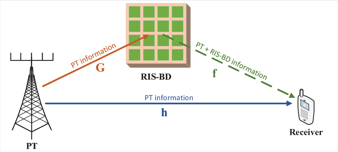
Fig. 1 shows a RIS-BD based MISO SR communication system, which includes an active PT with $M$ antennas, a passive RIS-BD with $N$ reflecting elements and a single-antenna receiver. Both the PT and RIS-BD wish to communicate with the receiver. The PT actively transmits its information-bearing signal to the receiver via multi-antenna beamforming. Meanwhile, the RIS-BD not only assists the primary transmission but also modulates its own information over the incident signal from the PT by cognitive backscattering communication technology. Thus, the RIS-BD reuses not only the spectrum, but also the power of the PT to transmit its own information.

Denote the MISO channel of the direct PT-to-receiver link as ${{\mathbf{h}}}=\left[{{h_{1}},\cdots,{h_{M}}}\right]^{\mathrm{T}}\in{\mathbb{C}^{M\times 1}}$, where $h_{m}$ is the channel coefficient between the $m$-th antenna of the PT and the receiver. Further, denote the channel matrix between the PT and RIS-BD as ${\mathbf{G}}=\left[{{g_{nm}}}\right]\in{\mathbb{C}^{N\times M}}$, where ${{g_{nm}}}$ is the channel coefficient between the $m$-th antenna of the PT and the $n$-th reflecting element of the RIS-BD. Moreover, the MISO channel of the RIS-BD-to-receiver link is denoted as ${{\mathbf{f}}}=\left[{{f_{1}},{f_{2}},\cdots,{f_{N}}}\right]^{\mathrm{T}}\in{\mathbb{C}^{N\times 1}}$, where ${{f_{n}}}$ is the channel coefficient between the $n$-th reflecting element of the RIS-BD and the receiver.

Since the RIS-BD operates as a low-power passive device, its own communication rate is much lower than that of the PT[34]. Therefore, we consider CSR setup, i.e., $T_{c}=L{T_{s}},L\gg 1$, where $T_{c}$ and $T_{s}$ is the symbol duration of the RIS-BD and the PT, respectively. Let $s\left(l\right)$ be the independent and identically distributed (i.i.d.) information-bearing symbol following the standard CSCG distribution, i.e., $s\left(l\right)\sim\mathcal{C}\mathcal{N}\left({0,1}\right)$. Further, denote $c\sim\mathcal{CN}(0,1)$ as the information-bearing symbol of the RIS-BD to be transmitted in one RIS-BD symbol period, which spans $L$ symbol periods of the primary signal $s\left(l\right)$, for $l=1,\cdots,L$. Further, denote the active transmit beamforming vector of the PT as ${\bf{w}}\in{{\mathbb{C}}^{M\times 1}}$, which satisfies ${\left\|{\mathbf{w}}\right\|^{2}}\leq P_{\max}$, with $P_{\max}$ denoting the maximum allowable transmit power of the PT.

Denote by ${\bm{\theta}}=\left[{\theta_{1}},\cdots,{\theta_{N}}\right]^{\mathrm{T}}\in{\mathbb{C}^{N\times 1}}$ the phase shift vector of the RIS-BD, where ${\theta_{n}}\in[0,2\pi)$ is the phase shift of the $n$-th reflecting element, for $n=1,...,N$. Let ${\bm{\phi}}=\left[{{e^{j{\theta_{1}}}},{e^{j{\theta_{2}}}},\cdots,{e^{j{\theta_{N}}}}}\right]^{\mathrm{H}}\in{\mathbb{C}^{N\times 1}}$ denote the reflection coefficient vector. Therefore, the reflected signal from the RIS-BD can be expressed as $\sqrt{\rho}{{\mathbf{f}}^{\mathrm{H}}}{\mathbf{\Phi Gw}}s\left(l\right)c$, where ${\mathbf{\Phi}}={\text{diag}}\left({\bm{\phi}}^{\mathrm{H}}\right)\in{\mathbb{C}^{N\times N}}$ is the reflection coefficient matrix of the RIS-BD, and $0<\rho\leq 1$ denotes the reflection efficiency.

The received signals at the receiver for each backscattering symbol period can be written as

where $l=1,\cdots,L$ and $z\left(l\right)\sim\mathcal{CN}\left({0,{\sigma^{2}}}\right)$ is the additive white Gaussian noise (AWGN) with zero mean and power ${\sigma^{2}}$.

The second term in (1) can be viewed as the output of the primary signal $s\left(l\right)$ passing through a channel $\sqrt{\rho}{{\mathbf{f}}^{\mathrm{H}}}{\mathbf{\Phi G}}c$ that varies depending on the passive backscattering signal $c$. Based on the received signal (1), the receiver first decodes the active primary signal $s\left(l\right)$ by treating the passive signal $c$ as a multi-path component, and the equivalent channel for decoding $s\left(l\right)$ is denoted by ${\mathbf{h}}_{\mathrm{eq}}^{\mathrm{H}}(c)={{\mathbf{h}}^{\mathrm{H}}}+\sqrt{\rho}{{\mathbf{f}}^{\mathrm{H}}}{\mathbf{\Phi G}}c$. Therefore, the signal-to-noise ratio (SNR) for decoding $s\left(l\right)$ at the RIS-BD with a given $c$ is

From (2), the expression of ${\gamma_{s}}\left(c\right)$ is related to the passively modulated signal of the RIS-BD $c$, which changes relatively fast compared to the channel variation[35]. Thus, by taking expectation over the random passive signal $c$, the average achievable rate of the primary transmission is

After decoding $s\left(l\right)$, the primary signal can be subtracted from (1) before decoding the passive signal $c$. Specifically, for each RIS-BD symbol period, we denote the primary signal, the noise and the intermediate signal after removing the primary signal in vector by ${\mathbf{s}}={[s(1),s(2),\cdots,s(L)]^{\mathrm{T}}}$, ${\mathbf{z}}={[z(1),z(2),\cdots,z(L)]^{\mathrm{T}}}$ and $\hat{\mathbf{y}}={[y(1),y(2),\cdots,y(L)]^{\mathrm{T}}}$. Then it follows from (1) that

With ${\mathbf{s}}$ decoded at the receiver, the maximal ratio combining (MRC) can be applied by pre-multiplying $\hat{\mathbf{y}}$ in (4) by $\frac{1}{{\sqrt{L}}}{{\mathbf{s}}^{\mathrm{H}}}$. For $L\gg 1$, due to the law of large numbers and the fact that the information-bearing symbols $s(l)$ are i.i.d. random variables with variance 1, we have $\frac{1}{L}{{\mathbf{s}}^{\mathrm{H}}}{\mathbf{s}}\to 1$. Therefore, the resulting signal can be obtained by

where $\tilde{{z}}=\frac{1}{{\sqrt{L}}}{{\mathbf{s}}^{\mathrm{H}}}{\mathbf{z}}$ is the resulting noise which can be shown to follow the distribution $\mathcal{CN}({0,{\sigma^{2}}})$. As a result, the achievable rate of the RIS-BD is

where the denominator ${L}$ accounts for the fact that in the CSR setup, only one RIS-BD symbol is transmitted during $L$ successive primary symbol periods, and the primary signal can be viewed as a spread-spectrum code with length $L$ for RIS-BD symbols. Therefore, the SNR for decoding RIS-BD symbol ${\gamma_{c}}$ is increased by $L$ times, at the cost of symbol rate decreased by $1/L$ as (6)[5].

The total power consumption of the PT for the considered RIS-BD based SR system is composed of the power consumed by the power amplifier, which is modelled to be proportional to the signal transmission power ${\left\|{\mathbf{w}}\right\|^{2}}$, as well as the circuit power consumed in the PT, denoted as $P_{s}$. Therefore, the total power consumption of the PT is ${P_{PT}}\triangleq\mu{\left\|{\mathbf{w}}\right\|^{2}}+{P_{s}}$, where $\mu>1$ denotes the inefficiency of the power amplifier at the PT. On the other hand, the RIS-BD does not consume power for signal transmission, since its reflectors are passive elements that do not actively transmit signal. The power dissipated at the RIS-BD with $N$ reflecting elements is modelled as ${P_{RIS-BD}}\triangleq N{P_{r}}$, where ${P_{r}}$ denotes the power consumption of each phase shifter.

We define the EE of the PT as the ratio of the primary communication rate to its power consumption, which can be expressed as

On the other hand, the EE of the RIS-BD is defined as the ratio of the backscattering communication rate to its power consumption, which can be expressed as

It is observed from (7)-(8) that the EEs of both PT and RIS-BD critically depend on the transmit beamforming vector $\bf{w}$ and reflection matrix at the RIS-BD ${\mathbf{\Phi}}$. By varying $\bf{w}$ and ${\mathbf{\Phi}}$, the complete EE region can be obtained, which is defined as the union of all EE pairs as

To explicitly reveal the fundamental relationship between active and passive communications, in this section, we first analyze the maximum individual EE for the PT and the RIS-BD to get some insights before characterizing the EE region.

In this section, we analyze the asymptotic performance of SR when the number of PT antennas $M$ or RIS-BD elements $N$ goes very large, to exploit the channel hardening effect for SR systems.

By using the Rician channel model, the PT-to-receiver link can be expressed as

which is composed of a deterministic LoS path and spatially uncorrelated NLoS path. For a typical RIS-BD deployment, the PT-to-RIS-BD link $\mathbf{G}$ and the RIS-BD-to-receiver link $\mathbf{f}$ can be modelled by Rician fading composed of a deterministic line-of-sight (LoS) path and spatially correlated non-LoS (NLoS) path:

where $\beta_{TS}$ and $\beta_{SR}$ are the large-scale path losses of the PT-to-RIS-BD link and the RIS-BD-to-receiver link, $K_{2}$ and $K_{3}$ are the Rician K-factors between the PT and RIS-BD and between RIS-BD and receiver, and $\mathbf{R}_{TS}\in$ $\mathbb{C}^{N\times N}$ and $\mathbf{R}_{SR}\in\mathbb{C}^{N\times N}$ are their spatial correlation matrices. Also, $\mathbf{G}_{LoS}\in\mathbb{C}^{N\times M}$ and $\mathbf{f}_{LoS}\in\mathbb{C}^{N\times 1}$ are the deterministic LoS components and $\mathbf{G}_{NLoS}\in\mathbb{C}^{N\times M}$ and $\mathbf{f}_{NLoS}\in\mathbb{C}^{N\times 1}$ are the NLoS components whose entries are i.i.d. complex Gaussian random variables with zero mean and unit variance. Under the above models, we study the asymptotic behavior of the maximum EE of the PT and the RIS-BD, respectively.

References

- [1] S. Wang, J. Xu, and Y. Zeng, “Characterizing the energy-efficiency region of symbiotic radio communications,” in IEEE Int. Conf. Wirel. Commun. Signal Process. (WCSP), Nov. 2022, pp. 336–341.
- [2] M. Latva-aho, K. Leppänen, F. Clazzer, and A. Munari, Key drivers and research challenges for 6G ubiquitous wireless intelligence, M. Latva-aho and K. Leppänen, Eds., 2020. [Online]. Available: https://elib.dlr.de/133477/
- [3] X. You et al., “Towards 6G wireless communication networks: vision, enabling technologies, and new paradigm shifts,” Sci. China-Inf. Sci., vol. 64, no. 1, Jan. 2021.
- [4] L. Zhang, Y.-C. Liang, and D. Niyato, “6G visions: Mobile ultra-broadband, super internet-of-things, and artificial intelligence,” China Commun., vol. 16, no. 8, pp. 1–14, Aug. 2019.
- [5] R. Long, Y.-C. Liang, H. Guo, G. Yang, and R. Zhang, “Symbiotic radio: A new communication paradigm for passive internet of things,” IEEE Internet Things J., vol. 7, no. 2, pp. 1350–1363, Feb. 2020.
- [6] Y.-C. Liang, K.-C. Chen, G. Y. Li, and P. Mahonen, “Cognitive radio networking and communications: an overview,” IEEE Trans. Veh. Technol., vol. 60, no. 7, pp. 3386–3407, Sep. 2011.
- [7] H. Guo, Y.-C. Liang, R. Long, and Q. Zhang, “Cooperative ambient backscatter system: A symbiotic radio paradigm for passive IoT,” IEEE Wirel. Commun. Lett., vol. 8, no. 4, pp. 1191–1194, Aug. 2019.
- [8] Y.-C. Liang, Q. Zhang, E. G. Larsson, and G. Y. Li, “Symbiotic radio: Cognitive backscattering communications for future wireless networks,” IEEE Trans. Cognit. Commun. Netw., vol. 6, no. 4, pp. 1242–1255, Dec. 2020.
- [9] M. Bilal Janjua and H. Arslan, “Survey on symbiotic radio: A paradigm shift in spectrum sharing and coexistence,” arXiv e-prints, p. arXiv:2111.08948, Nov. 2021.
- [10] R. Long, H. Guo, L. Zhang, and Y.-C. Liang, “Full-duplex backscatter communications in symbiotic radio systems,” IEEE Access, vol. 7, pp. 21 597–21 608, Feb. 2019.
- [11] H. Guo, Y.-C. Liang, R. Long, S. Xiao, and Q. Zhang, “Resource allocation for symbiotic radio system with fading channels,” IEEE Access, vol. 7, pp. 34 333–34 347, Mar. 2019.
- [12] Y. Guo, G. Wang, R. Xu, R. He, X. Wei, and C. Tellambura, “Capacity analysis for wireless symbiotic communication systems with BPSK tags under sensitivity constraint,” IEEE Commun. Lett., vol. 26, no. 1, pp. 44–48, Jan. 2022.
- [13] Z. Chu, W. Hao, P. Xiao, M. Khalily, and R. Tafazolli, “Resource allocations for symbiotic radio with finite blocklength backscatter link,” IEEE Internet Things J., vol. 7, no. 9, pp. 8192–8207, Sep. 2020.
- [14] J. Xu, Z. Dai, and Y. Zeng, “Enabling full mutualism for symbiotic radio with massive backscatter devices,” in Proc. IEEE Glob. Commun. Conf. (GLOBECOM), Dec. 2021, pp. 1–6.
- [15] ——, “MIMO symbiotic radio with massive passive devices: Asymptotic analysis and precoding optimization,” arXiv e-prints, p. arXiv:2206.13203, Jun. 2022.
- [16] H. Yang, Y. Ye, K. Liang, and X. Chu, “Energy efficiency maximization for symbiotic radio networks with multiple backscatter devices,” IEEE open J. Commun. Soc., vol. 2, pp. 1431–1444, Jun. 2021.
- [17] R. Long, Y.-C. Liang, Y. Pei, and E. G. Larsson, “Active-load assisted symbiotic radio system in cognitive radio network,” in IEEE Workshop Signal Process. Adv. Wireless Commun. (SPAWC), May 2020, pp. 1–5.
- [18] S. Gong, X. Lu, D. T. Hoang, D. Niyato, L. Shu, D. I. Kim, and Y.-C. Liang, “Toward smart wireless communications via intelligent reflecting surfaces: A contemporary survey,” IEEE Commun. Surv. Tutor., vol. 22, no. 4, pp. 2283–2314, Jan. 2020.
- [19] M. Di Renzo, A. Zappone, M. Debbah, M.-S. Alouini, C. Yuen, J. de Rosny, and S. Tretyakov, “Smart radio environments empowered by reconfigurable intelligent surfaces: How it works, state of research, and the road ahead,” IEEE J. Sel. Areas Commun., vol. 38, no. 11, pp. 2450–2525, Nov. 2020.
- [20] M. A. ElMossallamy, H. Zhang, L. Song, K. G. Seddik, Z. Han, and G. Y. Li, “Reconfigurable intelligent surfaces for wireless communications: Principles, challenges, and opportunities,” IEEE Trans. Cogn. Commun. Netw., vol. 6, no. 3, pp. 990–1002, Sep. 2020.
- [21] J. Yuan, Y.-C. Liang, J. Joung, G. Feng, and E. G. Larsson, “Intelligent reflecting surface-assisted cognitive radio system,” IEEE Trans. Commun., vol. 69, no. 1, pp. 675–687, Jan. 2021.
- [22] S. Zhang and R. Zhang, “Capacity characterization for intelligent reflecting surface aided MIMO communication,” IEEE J. Sel. Areas Commun., vol. 38, no. 8, pp. 1823–1838, Aug. 2020.
- [23] H. Lu, Y. Zeng, S. Jin, and R. Zhang, “Aerial intelligent reflecting surface: Joint placement and passive beamforming design with 3D beam flattening,” IEEE Trans. Wirel. Commun., vol. 20, no. 7, pp. 4128–4143, Jul. 2021.
- [24] T. Hou, Y. Liu, Z. Song, X. Sun, Y. Chen, and L. Hanzo, “Reconfigurable intelligent surface aided NOMA networks,” IEEE J. Sel. Areas Commun., vol. 38, no. 11, pp. 2575–2588, Nov. 2020.
- [25] X. Lei, M. Wu, F. Zhou, X. Tang, R. Q. Hu, and P. Fan, “Reconfigurable intelligent surface-based symbiotic radio for 6G: Design, challenges, and opportunities,” IEEE Wirel. Commun., vol. 28, no. 5, pp. 210–216, Oct. 2021.
- [26] X. Xu, Y.-C. Liang, G. Yang, and L. Zhao, “Reconfigurable intelligent surface empowered symbiotic radio over broadcasting signals,” IEEE Trans. Commun., vol. 69, no. 10, pp. 7003–7016, Oct. 2021.
- [27] H. Chen, G. Yang, and Y.-C. Liang, “Joint active and passive beamforming for reconfigurable intelligent surface enhanced symbiotic radio system,” IEEE Wirel. Commun. Lett., vol. 10, no. 5, pp. 1056–1060, May 2021.
- [28] Z. Tu, R. Long, and Y.-C. Liang, “Reconfigurable intelligent surface-enabled two-way backscatter communication in symbiotic radio,” in IEEE Int. Conf. Commun. (ICC), May 2022, pp. 3747–3752.
- [29] J. Ye, S. Guo, S. Dang, B. Shihada, and M.-S. Alouini, “On the capacity of reconfigurable intelligent surface assisted MIMO symbiotic communications,” IEEE Trans. Wirel. Commun., vol. 21, no. 3, pp. 1943–1959, Mar. 2022.
- [30] D. K. P. Asiedu and J.-H. Yun, “Multiuser NOMA with multiple reconfigurable intelligent surfaces for backscatter communication in a symbiotic cognitive radio network,” IEEE Trans. Veh. Technol., vol. 72, no. 4, pp. 5300–5316, Dec. 2023.
- [31] Q. Li, M. Wen, L. Xu, and K. Li, “Reconfigurable intelligent surface-aided number modulation for symbiotic active/passive transmission,” IEEE Internet Things J., pp. 1–1, Nov. 2022.
- [32] J. Li, X. Li, Y. Bi, and J. Ma, “Energy-efficient joint resource allocation with reconfigurable intelligent surfaces in symbiotic radio networks,” IEEE Trans. Cogn. Commun. Netw., pp. 1–1, Dec. 2022.
- [33] H. Peng, C.-Y. Ho, Y.-T. Lin, and L.-C. Wang, “Energy-efficient symbiotic radio using generalized benders decomposition,” in Proc. IEEE Veh. Technol. Conf. (VTC), Sep. 2022, pp. 1–5.
- [34] H. Zhou, Y.-C. Liang, X. Kang, and S. Sun, “Cooperative beamforming for large intelligent surface assisted symbiotic radios,” in Proc. IEEE Glob. Commun. Conf. (GLOBECOM), Dec. 2020, pp. 1–6.
- [35] Q. Zhang, Y.-C. Liang, and H. V. Poor, “Reconfigurable intelligent surface assisted MIMO symbiotic radio networks,” IEEE Trans. Commun., vol. 69, no. 7, pp. 4832–4846, Jul. 2021.
- [36] Z. Yang, M. Chen, W. Saad, W. Xu, M. Shikh-Bahaei, H. V. Poor, and S. Cui, “Energy-efficient wireless communications with distributed reconfigurable intelligent surfaces,” IEEE Trans. Wirel. Commun., vol. 21, no. 1, pp. 665–679, Jan. 2022.
- [37] M. Jung, W. Saad, M. Debbah, and C. S. Hong, “On the optimality of reconfigurable intelligent surfaces (RISs): Passive beamforming, modulation, and resource allocation,” IEEE Trans. Wirel. Commun., vol. 20, no. 7, pp. 4347–4363, Jul. 2021.
- [38] D. Yang, Q. Wu, Y. Zeng, and R. Zhang, “Energy trade-off in ground-to-UAV communication via trajectory design,” IEEE Trans. Veh. Technol., vol. 67, no. 7, pp. 6721–6726, Jul. 2018.
- [39] W. Huang, Y. Zeng, and Y. Huang, “Achievable rate region of MISO interference channel aided by intelligent reflecting surface,” IEEE Trans. Veh. Technol., vol. 69, no. 12, pp. 16 264–16 269, Dec. 2020.
- [40] M. Razaviyayn, “Successive Convex Approximation: Analysis and applications,” May 2014, https://hdl.handle.net/11299/163884.
- [41] M. Grant and S. Boyd, “CVX: Matlab software for disciplined convex programming, version 2.1,” http://cvxr.com/cvx, Mar. 2014.