Regularization techniques for inhomogeneous (spatial) point processes intensity and conditional intensity estimation

We consider spatial point processes in $\mathbb{R}^{d}$. For ease of exposition, we view a point process as a random locally finite subset $\mathbf{X}$ of a Borel set $S\subseteq\mathbb{R}^{d}$, $d\geq 1$. For readers interested in measure theoretical details, we refer to e.g. Møller and Waagepetersen 2003; Daley and Vere-Jones 2007 or Dereudre 2019. This setting implies the following facts. First, we consider simple point processes (two points cannot occur at the same location). Second, we exclude manifold-valued point processes (like circular or spherical point processes), and marked point processes, even if most of the concepts and methodologies presented hereafter exist or can be straightforwardly adapted to such contexts.

Thus, $\mathbf{X}\cap B$ stands for the restriction of $\mathbf{X}$ to a set $B\subseteq S$ and we let $|B|$ denote the volume of any bounded $B\subset S$. Local finiteness of $\mathbf{X}$ means that $\mathbf{X}\cap B$ is finite almost surely (a.s.), that is the number of points $N(B)$ of $\mathbf{X}\cap B$ is finite a.s., whenever $B$ is bounded. We let ${\cal N}$ stand for the state space consisting of the locally finite subsets (or point configurations) of $S$.

The distribution of $\mathbf{X}$ can be characterized by the finite-dimensional distributions of counting variables, or by the void probability, i.e. the probability to have no point in any compact set. However, these are usually not accessible and it is easier to summarize (and estimate) interpretable statistical measures such as intensity functions and conditional intensity functions. A more rigorous introduction on intensities, Palm intensities and conditional intensities and their links with reduced moment measures, Palm measures and reduced Campbell measures can be found in Coeurjolly and Lavancier 2019. To get quicker to the core of the paper, we introduce them through Campbell theorem and Georgii-Nguyen-Zessin formula which may be viewed as integrals characterizations.

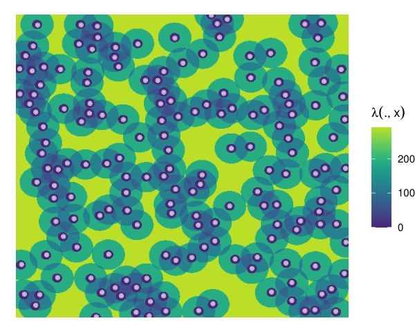
When $k=1$, we more simply speak of the intensity function or the Papangelou conditional intensity function. It is relevant to have the following interpretation of such functions: $\rho(u)$ (resp. $\lambda(u,\mathbf{X})$) can be interpreted as the probability to observe a point in $B(u,\mathrm{d}u)$ an infinitesimal ball centered at $u$ (resp. one point in $B(u,\mathrm{d}u)$ given the rest of the configuration of points outside the ball is $\mathbf{X}$). Similar interpretations are available when $k>1$. Equations (2.1)-(2.2) can be combined to show that $\rho(u)=\mathbb{E}\{\lambda(u,\mathbf{X})\}$ (also valid when $k>1$). Figure 1 illustrates briefly the functions $\rho$ and $\lambda$.

The reference model is the Poisson point process often defined as follows.

Poisson point processes model (eventually inhomogeneous) patterns with no interaction between points. As a consequence, it can be easily proved that for such processes, $\rho^{(k)}(u_{1},\dots,u_{k})=\lambda^{(k)}(\{u_{1},\dots,u_{k}\},\mathbf{X})=\prod_{i}\rho(u_{i})$. Large classes of models exist to introduce dependence between points. A survey can be found in Coeurjolly and Lavancier 2019 and the references therein. This is debatable but, to our point of view, the main classes are: Cox processes (which includes Neymann-Scott, shot noise Cox or log-Gaussian Cox processes, see e.g. Møller and Waagepetersen 2003) defined as Poisson point processes with random driven intensity obtained from a random field; Gibbs point processes (see Dereudre 2019), which are (in a bounded domain) defined via a density with respect to a Poisson point process with intensity 1; Determinantal point processes (e.g. Lavancier, Møller and Rubak 2015), for which intensities are defined through the determinant of a kernel function. We do not intend to define rigorously these models (see e.g. Coeurjolly and Lavancier 2019 and references therein), however it is worth pointing out that these models are very different by the kind of interaction they model, their flexibility and, in particular as regards the concern of this paper, the fact that the intensity function and/or the Papangelou conditional intensity function is explicit or not. Table 1 is an attempt to present the diversity of these models, their richness which also makes this research area attractive and fruitful.

Let us consider Figure 2 to motivate this section and paper. It is often the case in spatial statistics, that we observe a point pattern, here the locations of 3605 trees in a tropical forest (see Baddeley, Rubak and Turner 2015 for more details on this dataset) together with spatial covariates which are information available on the whole observation domain. A quick look at Figure 2 is enough to be convinced of the inhomogeneity (and maybe non independence) characteristic of the point pattern and that it makes completely sense to relate the distribution of trees with covariates such as the elevation, the slope of elevation or levels of soil nutrients.

In this application, we could be interested to model either the intensity and/or the Papangelou conditional intensity. We focus in this paper on exponential family models, where for any $u\in\mathbb{R}^{d}$ and $\mathbf{x}\in\mathcal{N}$

In both definitions, $\boldsymbol{\beta}=\{\beta_{1}(u),\dots,\beta_{p}(u)\}^{\top}\in\mathbb{R}^{p}$ represents the main vector parameter of interest, $\mathbf{z}(u)=\{z_{1}(u),\dots,z_{p}(u)\}^{\top},\;z_{i}:\mathbb{R}^{d}\to\mathbb{R}$ corresponds to the spatial covariates. We let $\boldsymbol{\psi}\in\mathbb{R}^{l}$ and $\mathbf{s}(u,\mathbf{x})=\{s_{1}(u,\mathbf{x}),\cdots,s_{l}(u,\mathbf{x})\}^{\top}$ denote the parameter and the sufficient statistics defining the interaction term (more details are given below). To rewrite (2.3) into the same formalism we suggest the reformulation

where $\boldsymbol{\beta}_{\rho}\in\mathbb{R}^{p}$ (resp. $\boldsymbol{\beta}_{\lambda}\in\mathbb{R}^{p+l}$), $\mathbf{z}_{\rho}(u)=\mathbf{z}(u)$ and $\mathbf{z}_{\lambda}(u,\mathbf{x})=\{\mathbf{z}(u)^{\top},\mathbf{s}(u,\mathbf{x})^{\top}\}^{\top}$. In the rest of the paper, each time we index a vector, matrix, random quantity by $\rho$ (resp. $\lambda$) means that we refer to the estimation of $\rho$ (resp. $\lambda$). And when a comment applies to the two problems, we write $\bullet$. Hence, for instance $\boldsymbol{\beta}_{\bullet}$ stands either for $\boldsymbol{\beta}_{\rho}$ or $\boldsymbol{\beta}_{\lambda}$. We point out that non-exponential family models can be considered but, as seen in Section 3.1, exponential models can be fitted very quickly using a tricky analogy with generalized linear models.

As a direct consequence of (2.4), the distribution of $\mathbf{X}$ is necessarily non-stationary. It is therefore highly relevant to ask the following questions: (A) given $\boldsymbol{\beta}_{\rho}$, $\mathbf{z}_{\rho}$, are there models with intensity $\rho$? (B) given $\boldsymbol{\beta}_{\lambda}$ and $\mathbf{z}_{\lambda}$, are there models with Papangelou conditional intensity $\lambda$. Answer to (A) is easy, as the Poisson point process already answers to this question. It is also quite simple to design inhomogeneous Cox point process or determinantal point process to achieve this task (see e.g. Choiruddin, Coeurjolly and Letué 2018; Lavancier, Møller and Rubak 2015). The question for (B) is much more complex (at least if $l\geq 1$, otherwise we are back to the Poisson case). As seen from Table 1, the question is essentially related to the existence of non-stationary Gibbs models. Dereudre, Drouilhet and Georgii 2012 (and the references therein) is one of the most popular existence result in the stationary case. In the non-stationary case, Vasseur, Coeurjolly and Dereudre 2020 provides sufficient conditions (which already cover a large class of examples): there exists at least one Gibbs measure with Papangelou conditional intensity $\lambda$ if it satisfies for any $u\in\mathbb{R}^{d}$ and $\mathbf{x}\in\mathcal{N}$

where $R,\bar{\lambda}<\infty$. The first part (finite range property) means that the Papangelou conditional intensity at $u$ depends only on points of $\mathbf{x}$ close to $u$. The second one, called local stability property, tells that the process is stochastically dominated by a Poisson point process. To set the ideas, the inhomogeneous Strauss model with $l=1$ and $s_{1}(u,\mathbf{x})=\sum_{v\in\mathbf{x}}\mathbf{1}(\|v-u\|\leq R)$ (number of $R$-closed neighbors of $u$ in $\mathbf{x}$) satisfies (2.5) for any $\psi\in[0,1]$ and $R<\infty$. We refer to Baddeley, Rubak and Turner 2015; Ba and Coeurjolly 2023 for more complex examples.

Hence, the problem of inferring $\rho$ or $\lambda$ given by (2.4) is a well-posed one. The aim of next sections is to estimate $\boldsymbol{\beta}_{\bullet}$ based on a single observation $\mathbf{x}$ in an observation domain say $D$ of $\mathbf{X}$, a spatial point process defined on $\mathbb{R}^{d}$ with intensity $\rho$ (or conditional intensity $\lambda$).

We consider composite likelihood-based techniques to estimate $\boldsymbol{\beta}_{\bullet}$. In particular we define the ($\log$-)Poisson likelihood and ($\log$-)pseudolikelihood respectively given by

where $D\ominus R$ in (3.2) stands for the domain eroded by the interaction range $R$. We use the the notation $\ell^{(1)}_{\bullet}$ and $\ell^{(2)}_{\bullet}$ to denote the gradient vector and the Hessian matrix with respect to $\boldsymbol{\beta}_{\bullet}$. In addition, our main result Theorem 2 requires the definition of $\mathbf{H}_{\bullet}(\boldsymbol{\beta}_{\bullet};\mathbf{X})=-\ell^{(2)}_{\bullet}(\mathbf{X};\boldsymbol{\beta}_{\bullet})$ which are given by

and we also define the matrix $\mathbf{H}_{\lambda}(\boldsymbol{\beta}_{\lambda})=\mathbb{E}\{\mathbf{H}_{\lambda}(\boldsymbol{\beta}_{\lambda};\mathbf{X})\}$.

Let us comment on these methodologies. We focus first on (3.1) to estimate $\rho$ given by (2.4). When $\mathbf{X}$ comes from a Poisson point process, as suggested by its name, (3.1) corresponds to the Poisson likelihood and its maximum was shown to converge by Rathbun and Cressie 1994. The method is still an efficient one for general models as the gradient of (3.1) is easily seen as an estimating equation by Campbell Theorem (2.1). Waagepetersen 2007 and then Waagepetersen and Guan 2009 proved asymptotic properties for general point processes under increasing domain asymptotic for large classes of mixing point processes. The efficiency of the method has been improved by Guan and Shen 2010 and then by Guan, Jalilian and Waagepetersen 2015 using quasi-likelihood. Infill asymptotic results have been obtained very recently by Choiruddin, Coeurjolly and Waagepetersen 2021.

Equation (3.2) has also an intuitive origin: Jensen and Møller 1991 obtained this criterion as the limit of a certain product of conditional densities. This paper together with Jensen and Künsch 1994 were also the first one to establish consistency and asymptotic normality for stationary exponential family Gibbs models satisfying (2.5) under the increasing domain framework. These results were extended by Billiot, Coeurjolly and Drouilhet 2008; Coeurjolly and Drouilhet 2010; Dereudre and Lavancier 2009 for more general models including infinite range pairwise interaction point processes or non-hereditary Gibbs models. Variant of the pseudo-likelihood include the Takacs-Fiksel method, the logistic regression likelihood and a form of quasi-likelihood respectively studied by Coeurjolly et al. 2012; Baddeley et al. 2014; Coeurjolly et al. 2016. The first results for inhomogeneous models were only proved very recently by Ba and Coeurjolly 2023, still in the increasing domain framework. The popularity of (3.1)-(3.2) lies without doubt by their simple implementation. This is discussed in the next section.

The main challenge to maximize (3.1)-(3.2) is the second term which involves an integral over the observation domain and needs to be approximated numerically. The Berman-Turner scheme Baddeley, Rubak and Turner 2015 is the popular approach conducted by discretizing the integral using both quadrature points and data points by

where $u_{i},i=1,\ldots,N+M$ are quadrature points in $D$ or $D\ominus R$ (depending on the problem) involving $N$ data points and $M$ dummy points and where the $w(u_{i})>0$ are quadrature weights such that ${\sum_{i}w(u_{i})}=|D|$ (or $|D\ominus R|$). Using this technique, (3.1)-(3.2) are then approximated by

where $w_{i}=w(u_{i}),y_{i}=w_{i}^{-1}\mathbf{1}(u_{i}\in{\mathbf{x}\cap D})$ (or $D\ominus R$), $\rho_{i}(\boldsymbol{\beta}_{\rho})=\rho(u_{i};\boldsymbol{\beta}_{\rho})$ and $\lambda_{i}(\boldsymbol{\beta}_{\lambda})=\lambda(u_{i},\mathbf{x};\boldsymbol{\beta}_{\rho})$. It is now relevant to remark that Equations (3.5)-(3.6) are equivalent to a weighted quasi-likelihood function of independent Poisson variables $y_{i}$ with weights $w_{i}$. Therefore, the implementation can take advantage of any software implementing generalized linear models. These methods are in particular implemented in the spatstat R package Baddeley, Rubak and Turner 2015. The accuracy of the approximation of $\ell_{\bullet}$ by $\tilde{\ell}_{\bullet}$ increases when $N$ is small with respect to $M$. If $N$ is too large or if increasing $M$ leads to numerical instabilities, the induced bias can be non negligible. In these situations, alternatives based on the use of an approximation of (3.1)-(3.2) by a logistic regression likelihood are available (see e.g. Waagepetersen 2007; Baddeley et al. 2014).

To sum up Section 3: when $p$ is moderate, we have at our disposal a bunch of statistical methodologies to estimate either the intensity or conditional intensity function. These methodologies are well-studied from a mathematical point of view and efficiently implemented.

The application summarized by Figure 2 suggests that more refined methods are necessary. The number of spatial covariates is large (close to 100 if one considers topographic, levels of soil nutrients and levels of combinations of soil nutrients) which leads to numerical problems if one considers methods described in Section 3.1. Known as the curse of dimensionality, these problems can be alleviated if one assumes sparsity in the intensity model and makes use of regularized versions of (3.1)-(3.2).

Let us turn to the setting of the present paper. We assume that we observe one realization from $\mathbf{X}_{n}$ where $(\mathbf{X}_{n})_{n\geq 1}$ is a sequence of point processes defined in $\mathbb{R}^{d}$ and observed in $D_{n}$. We assume that either the intensity $\rho$ or the Papangelou conditional intensity $\lambda$ is modelled by (2.4). The true parameter (to be estimated) is denoted by $\boldsymbol{\beta}_{0,\bullet}$ and we assume it can be decomposed as $\boldsymbol{\beta}_{0,\rho}=(\boldsymbol{\beta}_{01,\rho}^{\top},\boldsymbol{\beta}_{02,\rho}^{\top})^{\top}$ and $\boldsymbol{\beta}_{0,\lambda}=(\boldsymbol{\beta}_{01,\lambda}^{\top},\boldsymbol{\beta}_{02,\lambda}^{\top},\boldsymbol{\psi})^{\top}$ where $\boldsymbol{\beta}_{01,\bullet}=0$ and where all components of $\boldsymbol{\beta}_{02,\bullet}$ are non zero. We index any (random) vector, matrix in the same way. Thus $\mathbf{z}_{01,\bullet}$ corresponds to the set of non-informative covariates while the set $\mathbf{z}_{02,\bullet}$ represents the set of active features. We assume that $\boldsymbol{\beta}_{02,\rho}$ or $(\boldsymbol{\beta}_{02,\lambda}^{\top},\boldsymbol{\psi}^{\top})^{\top}$ has length $s_{n}$. Thus $\boldsymbol{\beta}_{01,\bullet}$ has length $p_{n}-s_{n}$. The sequences $s_{n}$ and $p_{n}$ may increase with $n$. Finally, to quantify the amount of increase of data with $n$, we assume for both problems that $\rho,\lambda$, $\boldsymbol{\beta}_{0,\bullet}$ and $D_{n}$ are such that $\mu_{n}\to\infty$ as $n\to\infty$

We assume that for any $n\geq 1$, the model is well-defined. In particular for $\lambda$, this means the sequence of Papangelou conditional intensity functions satisfies (2.5). Note that $\mu_{n}$ is a function of $D_{n},\boldsymbol{\beta}_{01},\mathbf{z}_{1,\bullet}(u)$ and $s_{n}$. We believe this kind of framework is original and quite general. It embraces the well-known frameworks called increasing domain asymptotics and infill asymptotics. For the increasing domain context, $D_{n}\to\mathbb{R}^{d}$ and usually $\boldsymbol{\beta}_{02,\dots}$ depends only on $n$ through $s_{n}$. For the infill asymptotics, $D_{n}=D$ is assumed to be a bounded domain of $\mathbb{R}^{d}$ and usually $(\mathbf{z}_{2})_{1}(u)=1$, $(\boldsymbol{\beta}_{02,\bullet})_{1}=\theta_{n}\to\infty$ as $n\to\infty$. In some sense, the parameter $\mu_{n}$ plays the role of the sample size in standard inference. To reduce notation in the following, unless it is ambiguous, we do not index $\mathbf{X}$, $\rho$, $\lambda$, $\boldsymbol{\beta}_{0}$, $\boldsymbol{\beta}$, $\mathbf{z}_{\bullet}(u),\ell_{\bullet}$ with $n$.

When the number of parameters is large, regularization methods allow one to perform both estimation and variable selection simultaneously. When $p_{n}=p$, Choiruddin, Coeurjolly and Letué 2018 consider several regularization procedures which consist in adding a convex or non-convex penalty term to (3.1)-(3.2). A quite similar approach was considered in Ba and Coeurjolly 2023 for Gibbs point processes. To ease the presentation and focus more on the similarities between the two problems of inferring (2.4), we only consider the $\ell^{1}$ regularization which gives rise to the adaptive lasso procedure. The $\ell^{1}$-regularized versions of (3.1)-(3.2) are given by

where the real numbers $\tau_{n,j}$ are non-negative tuning parameters. The adaptive lasso estimator is then defined by

When $\tau_{n,j}=0$ for $j=1,\dots,p_{n}$, the method reduces to the maximum Poisson likelihood or pseudo-likelihood estimator and when $\tau_{n,j}=\tau_{n}$ to the standard lasso estimator. Note that in the formulation (4.2), if we want the model to necessarily have an intercept term and/or if one does not want to regularize the parameter vector corresponding to the interaction term for $\lambda$, we can simply set the corresponding tuning parameters to 0. The choice of $\mu_{n}$ as a normalization factor in (4.2) follows the implementation of the adaptive lasso procedure for generalized linear models in the standard software (e.g. R package glmnet Friedman, Hastie and Tibshirani 2010).

Our result relies upon the following conditions:

1. 1.

   For any $n\geq 1$, the intensity or the conditional intensity functions has the log-linear specification given by (2.4) where $\boldsymbol{\beta}_{\bullet}\in\mathbb{R}^{p_{n}}$. For $\lambda$, we assume that it satisfies (2.5).

2. 2.

   $(\mu_{n})_{n\geq 1}$ is an increasing sequence of real numbers, such that $\mu_{n}\to\infty$ as ${n}\to\infty$.

3. 3.

   As $n\to\infty$, $\ell^{(1)}_{\bullet}(\boldsymbol{\beta}_{0,\bullet};\mathbf{X})=O_{\mathrm{P}}\left(\sqrt{p_{n}\mu_{n}}\right)$.

4. 4.

   The matrix $\mathbf{H}_{\rho}(\boldsymbol{\beta}_{0,\rho})$ or the matrices $\mathbf{H}_{\lambda}(\boldsymbol{\beta}_{0,\lambda};\mathbf{X})$ and $\mathbf{H}_{\lambda}(\boldsymbol{\beta}_{0,\lambda})$ satisfy

   $$\inf_{n\geq 1}\inf_{\boldsymbol{\phi}\in\mathbb{R}^{p_{n}},\|\boldsymbol{\phi}\|=1}\mu_{n}^{-1}\boldsymbol{\phi}^{\top}\mathbf{H}_{\bullet}(\boldsymbol{\beta}_{0,\bullet})\boldsymbol{\phi}>0\quad\text{ and }$$

   $$\sup_{\boldsymbol{\phi}\in\mathbb{R}^{p_{n}},\|\boldsymbol{\phi}\|=1}\boldsymbol{\phi}^{\top}\left\{\mathbf{H}_{\lambda}(\boldsymbol{\beta}_{0,\lambda};\mathbf{X})-\mathbf{H}_{\lambda}(\boldsymbol{\beta}_{0,\lambda}\right\}\boldsymbol{\phi}=o_{\mathrm{P}}(\mu_{n}).$$

5. 5.

   As $n\to\infty$, $p_{n}^{4}/\mu_{n}\to 0$.

6. 6.

   For any $c\in\mathbb{R}$, $\tilde{\boldsymbol{\beta}}_{\bullet}=\boldsymbol{\beta}_{0,\bullet}+c\sqrt{p_{n}/\mu_{n}}$ and $j=1,\dots,p_{n}-s_{n}$

   $\displaystyle\int_{D_{n}}\|\mathbf{z}_{\rho}(u)\|^{3}\rho(u;\tilde{\boldsymbol{\beta}}_{\rho})\mathrm{d}u=O(p_{n}^{3/2}),$

   $$\int_{D_{n}\ominus R}\|\mathbf{z}_{\lambda}(u,\mathbf{X})\|^{3}\lambda(u,\mathbf{X};\tilde{\boldsymbol{\beta}}_{\lambda})\mathrm{d}u=O_{\mathrm{P}}(p_{n}^{3/2}),$$

   $$\int_{D_{n}}|(\mathbf{z}_{\rho})_{j}(u)|\|\mathbf{z}_{\rho}(u)\|\rho(u;\tilde{\boldsymbol{\beta}}_{\rho})\mathrm{d}u=O(\sqrt{p_{n}})\quad\text{ and }$$

   $$\int_{D_{n}\ominus R}|(\mathbf{z}_{\lambda})_{j}(u,\mathbf{X})|\|\mathbf{z}_{\lambda}(u,\mathbf{X})\|\lambda(u,\mathbf{X};\tilde{\boldsymbol{\beta}}_{\lambda})\mathrm{d}u=O_{\mathrm{P}}(\sqrt{p_{n}}).$$

7. 7.

   Let $a_{n}=\max_{j=p_{n}-s_{n}+1,\ldots,{p_{n}}}\tau_{n,j}$ and $b_{n}=\min_{j={1},\ldots,p_{n}-s_{n}}\tau_{n,j}$. The $\tau_{n,j}$ are allowed to be stochastic and we assume that, as $n\to\infty$

   $\displaystyle a_{n}\sqrt{\frac{s_{n}\mu_{n}}{p_{n}}}=o_{\mathrm{P}}(1)\qquad\text{ and }\qquad\frac{1}{b_{n}}\sqrt{\frac{p_{n}^{2}}{\mu_{n}}}=o_{\mathrm{P}}(1).$

Let us discuss these conditions. Conditions 1-2 have already been explained. It is worth saying that in an attempt to embrace both problems of estimating $\rho$ or $\lambda$ (and ease the presentation) some conditions may appear useless or too vague. This is the case for 3, 4 and 6. We invite the reader to refer to Choiruddin, Coeurjolly and Letué 2023; Ba and Coeurjolly 2023 where conditions on second-order moments (for $\rho$) or second-order Papangelou conditional intensity (for $\lambda$ and in the increasing domain framework) are presented. Essentially, condition 3 is obtained by proving that the variance of the score behaves as $p_{n}\mu_{n}$ (which corresponds to $np_{n}$ for standard GLMs for instance). Condition 4 shows that the smallest eigenvalue of $\mu_{n}^{-1}\mathbf{H}_{\bullet}(\boldsymbol{\beta}_{0,\bullet})$ is positive for any $n$ and could be compared to an assumption of the form $n^{-1}\mathbf{X}\mathbf{X}^{\top}$ tends to a positive definite matrix for standard linear models with fixed number of covariates (where $\mathbf{X}$ would stand for the design matrix). Condition 6 looks meaningless however, for instance for $\rho$ and $c=0$, these are fulfilled as soon as $\sup_{n}\sup_{i}\sup_{u}|(\mathbf{z})_{i}(u)|<\infty$ (again see Choiruddin, Coeurjolly and Letué 2023; Ba and Coeurjolly 2023 for more details). Condition 5 is one of the most important and provides a restriction on the number of covariates. Condition 7 expresses the compromise to be considered on $s_{n},p_{n},\mu_{n}$ and the regularization parameters to ensure consistency and oracle properties. These are quite similar to the corresponding ones considered by Choiruddin, Coeurjolly and Letué 2023; Ba and Coeurjolly 2023. We include here the possibility to have stochastic regularization parameters. Condition 7 shows the interest of the adaptive lasso. Indeed for the standard lasso $a_{n}=b_{n}$ and both conditions cannot be fulfilled simultaneously even if $s_{n}$ and $p_{n}$ do not depend on $n$.

A look at the proof of Theorem 2(i) shows in particular that the consistency remains true under the first part of condition 7 and so remains valid for the standard lasso and actually even if no regularization is considered. The combination of Theorem 2 (i)-(ii) justifies the interest of a regularization technique. With the same rate of convergence than the one of the unregularized estimator, we ensure that the parameters estimates for non-informative covariates can be set to 0 with probability tending to 1.

We decided not to include more results to keep the paper readable and short. Choiruddin, Coeurjolly and Letué 2023; Ba and Coeurjolly 2023 explore for example the asymptotic normality of $\hat{\boldsymbol{\beta}}_{2,\rho}$ and $(\hat{\boldsymbol{\beta}}_{2,\lambda}^{\top},\hat{\boldsymbol{\psi}}^{\top})^{\top}$ respectively, and estimates of asymptotic covariance matrices. In the same vein, we only focus on the adaptive lasso penalty. More convex penalties (e.g. adaptive elastic net) as well as non-convex penalties (such as MC+, SCAD penalties) are considered in aforementioned references.

Theorem 2 extends the results obtained by Choiruddin, Coeurjolly and Letué 2023; Ba and Coeurjolly 2023. In particular for the estimation problem of $\lambda$, we consider the possibility to include an infill asymptotics and we allow the number of parameters for the interaction parameter, that is the length of $\boldsymbol{\psi}$, to increase with $n$. For both problems, we allow the tuning parameters to be stochastic, see Section 4.3 and this of great interest. Indeed, Zou and Zhang 2009 and many authors after this work suggest to scale the regularization parameters as $\tau_{n,j}=\tau_{n}/|(\check{\boldsymbol{\beta}}_{\bullet})_{j}|^{\gamma}$ where $\tau_{n}$ is a non-negative sequence, $\gamma>0$ and where $\check{\boldsymbol{\beta}}_{\bullet}$ is the unregularized estimator (or actually any estimate producing no zero). This popular idea is indeed very natural as it is expected that the $\tau_{n,j}$ for the non-informative covariates will be much larger than the ones for the informative ones and so estimates of parameters corresponding to non-informative covariates will be more likely set to zero thanks to the $\ell^{1}$ penalty. We claim that $\tau_{n}$ can be adjusted to fulfill condition 7. Indeed, since $(\check{\boldsymbol{\beta}}_{\bullet})_{j}-(\boldsymbol{\beta}_{0,\bullet})_{j}=O_{\mathrm{P}}(\sqrt{p_{n}/\mu_{n}})$, it is easily deduced that $a_{n}=O_{\mathrm{P}}(\tau_{n})$ and $b_{n}^{-1}=\max_{j\leq p_{n}-s_{n}}\tau_{n,j}^{-1}=O_{\mathrm{P}}\{\tau_{n}^{-1}(p_{n}/\mu_{n})^{\gamma/2}\}$. Now, since $s_{n}\leq p_{n}$ and $p_{n}^{4}/\mu_{n}=o(1)$ by condition 5,

And so condition 7 is in particular satisfied if $\tau_{n}\sqrt{\mu_{n}}\to 0$ and $\tau_{n}\mu_{n}^{1/4+3\gamma/8}\to\infty$ as $n\to\infty$. For instance, if $\tau_{n}=\mu_{n}^{-\alpha}$ with $\alpha>0$, this imposes the non-empty condition $1/2<\alpha<1/4+3\gamma/8$ (if $\gamma>2/3$). A discussion on how to select $\tau_{n}$ and/or $\gamma$ and other numerical considerations are presented in the next section.

To implement regularization methods for spatial point processes in particular within R, we combine the existing R package spatstat Baddeley, Rubak and Turner 2015 (devoted to the analysis of spatial point pattern data) with two R packages glmnet Friedman, Hastie and Tibshirani 2010 (for convex penalties) and ncvreg Breheny and Huang 2011 (for non-convex penalties) which use coordinate descent procedures/algorithms Friedman, Hastie and Tibshirani 2010; Breheny and Huang 2011; Choiruddin, Coeurjolly and Letué 2018; Daniel, Horrocks and Umphrey 2018. Those methods rely on the tuning parameters $\tau_{n,j}$. Following Zou and Zhang 2009, we suggest to use $\tau_{n,j}=\tau_{n}/|(\check{\boldsymbol{\beta}}_{\bullet})_{j}|^{\gamma}$ where $\tau=\tau_{n}$ is to be chosen (the parameter $\gamma$ has lesss influence and is often set to 1). Large values of $\tau$ yield estimates with high biases and low variances, whereas small values of $\tau$ produce estimates with low biases and high variances. Therefore, an optimal choice of the tuning parameter $\tau$ is necessary to control the trade-off between the bias and the variance. To select $\tau$, it is reasonable first to identify a decreasing sequence of $\tau$ ranging from a maximum value of $\tau$ for which all penalized coefficients are zero to $\tau=0$ (which corresponds to the unregularized parameter estimates); and second to define a criterion to select $\tau$ by an optimization (minimization) procedure. Following Choiruddin, Coeurjolly and Waagepetersen 2021; Ba and Coeurjolly 2023, we suggest the use of an information criteria such as the (composite) Bayesian information criterion (BIC) Schwarz 1978; Gao and Song 2010 or the (composite) extended regularized information criterion (ERIC) Hui, Warton and Foster 2015 to select $\tau$. Let us define first the (composite) BIC, which we denote by cBIC,

where $N$ is the observed number of points and

with $\boldsymbol{\Sigma}_{\bullet}(\boldsymbol{\beta}_{\bullet})=\mathbf{H}_{\bullet}(\boldsymbol{\beta}_{\bullet})^{-1}\mathbf{V}_{\bullet}(\boldsymbol{\beta}_{\bullet})\mathbf{H}_{\bullet}(\boldsymbol{\beta}_{\bullet})^{-1}$ and $\mathbf{V}_{\bullet}(\boldsymbol{\beta}_{\bullet})=\mathrm{Var}(\ell^{(1)}_{\bullet}(\boldsymbol{\beta}_{\bullet};\mathbf{X}))$. It is worth pointing out that $d(\tau)$ is called the effective number of parameters in the model with tuning parameter $\tau$ and for models with tractable likelihood functions like the inhomogeneous Poisson point process, $d(\tau)$ corresponds to the number of non-zero coefficients in $\hat{\boldsymbol{\beta}}_{\bullet}$ and the criterion reduces to BIC. For Gibbs models, estimates of $\mathbf{H}_{\lambda}$ and $\boldsymbol{\Sigma}_{\lambda}$ can be efficiently computed using the vcov function of the spatstat R package Coeurjolly and Rubak 2013. Let us now define the (composite) ERIC, which we denote by cERIC and which is designed for the purpose of taking into account the effects of the tuning parameter $\tau$,

To sum up, we choose the tuning parameter $\tau\geq 0$ which minimizes either cBIC or cERIC. For more numerical details as well as implementation of the methodology, we refer the reader to Ba and Coeurjolly 2023; Choiruddin, Coeurjolly and Letué 2018; Choiruddin, Coeurjolly and Waagepetersen 2021; Choiruddin et al. 2023. We end this section by mentioning that a recent version of the spatstat R package allows to include elastic regularization in the ppm function through the option improve.type=‘‘enet’’.

References

- Ba and Coeurjolly (2023) [author] Ba, IsmaïlaI. and Coeurjolly, Jean-FrançoisJ.-F. (2023). Inference for low-and high-dimensional inhomogeneous Gibbs point processes. to appear in Scandinavian Journal of Statistics.
- Baddeley, Rubak and Turner (2015) [author] Baddeley, AdrianA., Rubak, EgeE. and Turner, RolfR. (2015). Spatial point patterns: methodology and applications with R. Chapman and Hall/CRC.
- Baddeley et al. (2014) [author] Baddeley, AdrianA., Coeurjolly, Jean-FrançoisJ.-F., Rubak, EgeE. and Waagepetersen, RasmusR. (2014). Logistic regression for spatial Gibbs point processes. Biometrika 101 377–392.
- Billiot, Coeurjolly and Drouilhet (2008) [author] Billiot, Jean-MichelJ.-M., Coeurjolly, Jean-FrançoisJ.-F. and Drouilhet, RémyR. (2008). Maximum pseudolikelihood estimator for exponential family models of marked Gibbs point processes. Electronic Journal of Statistics 2 243–264.
- Breheny and Huang (2011) [author] Breheny, PatrickP. and Huang, JianJ. (2011). Coordinate descent algorithms for nonconvex penalized regression, with applications to biological feature selection. The Annals of Applied Statistics 5 232.
- Choiruddin, Coeurjolly and Letué (2018) [author] Choiruddin, AchmadA., Coeurjolly, Jean-FrançoisJ.-F. and Letué, FrédériqueF. (2018). Convex and non-convex regularization methods for spatial point processes intensity estimation. Electronic Journal of Statistics 12 1210–1255.
- Choiruddin, Coeurjolly and Waagepetersen (2021) [author] Choiruddin, AchmadA., Coeurjolly, Jean-FrançoisJ.-F. and Waagepetersen, RasmusR. (2021). Information criteria for inhomogeneous spatial point processes. Australian & New Zealand Journal of Statistics 63 119–143.
- Choiruddin, Coeurjolly and Letué (2023) [author] Choiruddin, AchmadA., Coeurjolly, Jean-FrançoisJ.-F. and Letué, FrédériqueF. (2023). Adaptive lasso and Dantzig selector for spatial point processes intensity estimation. Bernoulli 29 1849–1876.
- Choiruddin et al. (2023) [author] Choiruddin, AchmadA., Susanto, Tabita YuniT. Y., Husain, AhmadA. and Kartikasari, Yuniar MegaY. M. (2023). kppmenet: Combining the kppm and elastic net regularization for inhomogeneous Cox point process with correlated covariates. Journal of Applied Statistics 1–14.
- Coeurjolly and Drouilhet (2010) [author] Coeurjolly, Jean-FrançoisJ.-F. and Drouilhet, RémyR. (2010). Asymptotic properties of the maximum pseudo-likelihood estimator for stationary Gibbs point processes including the Lennard-Jones model. Electronic Journal of Statistics 4 677–706.
- Coeurjolly and Lavancier (2019) [author] Coeurjolly, Jean-FrançoisJ.-F. and Lavancier, FrédéricF. (2019). Understanding Spatial Point Patterns Through Intensity and Conditional Intensities. In Stochastic Geometry.. Lecture Notes in Mathematics 2237 45-85.
- Coeurjolly and Rubak (2013) [author] Coeurjolly, Jean-FrançoisJ.-F. and Rubak, EgeE. (2013). Fast covariance estimation for innovations computed from a spatial Gibbs point process. Scandinavian Journal of Statistics 40 669–684.
- Coeurjolly et al. (2012) [author] Coeurjolly, Jean-FrançoisJ.-F., Dereudre, DavidD., Drouilhet, RémyR. and Lavancier, FrédéricF. (2012). Takacs–Fiksel method for stationary marked Gibbs point processes. Scandinavian Journal of Statistics 39 416–443.
- Coeurjolly et al. (2016) [author] Coeurjolly, Jean-FrançoisJ.-F., Guan, YongtaoY., Khanmohammadi, MahdiehM. and Waagepetersen, RasmusR. (2016). Towards optimal Takacs–Fiksel estimation. Spatial Statistics 18 396–411.
- Daley and Vere-Jones (2007) [author] Daley, Daryl JD. J. and Vere-Jones, DavidD. (2007). An introduction to the theory of point processes: volume II: general theory and structure. Springer Science & Business Media.
- Daniel, Horrocks and Umphrey (2018) [author] Daniel, JeffreyJ., Horrocks, JulieJ. and Umphrey, Gary JG. J. (2018). Penalized composite likelihoods for inhomogeneous Gibbs point process models. Computational Statistics & Data Analysis 124 104–116.
- Dereudre (2019) [author] Dereudre, DavidD. (2019). Introduction to the theory of Gibbs point processes. In Springer Lecture Notes in Stochastic Geometry 181–229. Springer.
- Dereudre, Drouilhet and Georgii (2012) [author] Dereudre, DavidD., Drouilhet, RémyR. and Georgii, Hans-OttoH.-O. (2012). Existence of Gibbsian point processes with geometry-dependent interactions. Probability Theory and Related Fields 153 643–670.
- Dereudre and Lavancier (2009) [author] Dereudre, DavidD. and Lavancier, FrédéricF. (2009). Campbell equilibrium equation and pseudo-likelihood estimation for non-hereditary Gibbs point processes. Bernoulli 15 1368–1396.
- Friedman, Hastie and Tibshirani (2010) [author] Friedman, JeromeJ., Hastie, TrevorT. and Tibshirani, RobR. (2010). Regularization paths for generalized linear models via coordinate descent. Journal of Statistical Software 33 1.
- Gao and Song (2010) [author] Gao, XinX. and Song, Peter X-KP. X.-K. (2010). Composite likelihood Bayesian information criteria for model selection in high-dimensional data. Journal of the American Statistical Association 105 1531–1540.
- Guan, Jalilian and Waagepetersen (2015) [author] Guan, YongtaoY., Jalilian, AbdollahA. and Waagepetersen, RasmusR. (2015). Quasi-likelihood for spatial point processes. Journal of the Royal Statistical Society. Series B, Statistical methodology 77 677.
- Guan and Shen (2010) [author] Guan, YongtaoY. and Shen, YeY. (2010). A weighted estimating equation approach for inhomogeneous spatial point processes. Biometrika 97 867–880.
- Hui, Warton and Foster (2015) [author] Hui, Francis KCF. K., Warton, David ID. I. and Foster, Scott DS. D. (2015). Tuning parameter selection for the adaptive lasso using ERIC. Journal of the American Statistical Association 110 262–269.
- Illian et al. (2008) [author] Illian, JanineJ., Penttinen, AnttiA., Stoyan, HelgaH. and Stoyan, DietrichD. (2008). Statistical analysis and modelling of spatial point patterns 70. John Wiley & Sons.
- Jensen and Künsch (1994) [author] Jensen, Jens LedetJ. L. and Künsch, Hans RH. R. (1994). On asymptotic normality of pseudo likelihood estimates for pairwise interaction processes. Annals of the Institute of Statistical Mathematics 46 475–486.
- Jensen and Møller (1991) [author] Jensen, Jens LedetJ. L. and Møller, JesperJ. (1991). Pseudolikelihood for exponential family models of spatial point processes. The Annals of Applied Probability 1 445–461.
- Lavancier, Møller and Rubak (2015) [author] Lavancier, FrédéricF., Møller, JesperJ. and Rubak, EgeE. (2015). Determinantal point process models and statistical inference. Journal of the Royal Statistical Society: Series B: Statistical Methodology 853–877.
- Møller and Waagepetersen (2003) [author] Møller, JesperJ. and Waagepetersen, Rasmus PlengeR. P. (2003). Statistical inference and simulation for spatial point processes. Chapman and Hall/CRC.
- Rathbun and Cressie (1994) [author] Rathbun, Stephen LS. L. and Cressie, NoelN. (1994). Asymptotic properties of estimators for the parameters of spatial inhomogeneous Poisson point processes. Advances in Applied Probability 26 122–154.
- Schwarz (1978) [author] Schwarz, GideonG. (1978). Estimating the dimension of a model. The Annals of Statistics 6 461–464.
- Thurman and Zhu (2014) [author] Thurman, Andrew LA. L. and Zhu, JunJ. (2014). Variable selection for spatial Poisson point processes via a regularization method. Statistical Methodology 17 113–125.
- Thurman et al. (2015) [author] Thurman, Andrew LA. L., Fu, RaoR., Guan, YongtaoY. and Zhu, JunJ. (2015). Regularized estimating equations for model selection of clustered spatial point processes. Statistica Sinica 173–188.
- Vasseur, Coeurjolly and Dereudre (2020) [author] Vasseur, ThibaultT., Coeurjolly, Jean-FrançoisJ.-F. and Dereudre, DavidD. (2020). Existence of inhomogeneous Gibbs point processes in the infinite volume. Preprint.
- Waagepetersen (2007) [author] Waagepetersen, Rasmus PlengeR. P. (2007). An estimating function approach to inference for inhomogeneous Neyman–Scott processes. Biometrics 63 252–258.
- Waagepetersen and Guan (2009) [author] Waagepetersen, RasmusR. and Guan, YongtaoY. (2009). Two-step estimation for inhomogeneous spatial point processes. Journal of the Royal Statistical Society: Series B (Statistical Methodology) 71 685–702.
- Zou and Zhang (2009) [author] Zou, HuiH. and Zhang, Hao HelenH. H. (2009). On the adaptive elastic-net with a diverging number of parameters. The Annals of Statistics 37 1733.