The First Proven Performance Guarantees for the
Non-Dominated Sorting Genetic Algorithm II (NSGA-II)
on a Combinatorial Optimization ProblemThanks: Author-generated version of a paper appearing in the proceedings of IJCAI 2023.Work done while visiting École Poytechnique, France.
Abstract
The Non-dominated Sorting Genetic Algorithm-II (NSGA-II) is one of the most prominent algorithms to solve multi-objective optimization problems. Recently, the first mathematical runtime guarantees have been obtained for this algorithm, however only for synthetic benchmark problems.
In this work, we give the first proven performance guarantees for a classic optimization problem, the NP-complete bi-objective minimum spanning tree problem. More specifically, we show that the NSGA-II with population size computes all extremal points of the Pareto front in an expected number of iterations, where is the number of vertices, the number of edges, and is the maximum edge weight in the problem instance. This result confirms, via mathematical means, the good performance of the NSGA-II observed empirically. It also shows that mathematical analyses of this algorithm are not only possible for synthetic benchmark problems, but also for more complex combinatorial optimization problems.
As a side result, we also obtain a new analysis of the performance of the global SEMO algorithm on the bi-objective minimum spanning tree problem, which improves the previous best result by a factor of , the number of extremal points of the Pareto front, a set that can be as large as . The main reason for this improvement is our observation that both multi-objective evolutionary algorithms find the different extremal points in parallel rather than sequentially, as assumed in the previous proofs.
1 Introduction
Many optimization problems consist of several conflicting objectives. In such a situation, it is not possible to compute a single optimal solution. The most common solution concept therefore is to compute a set of Pareto optima (solutions which cannot be improved in one objective without accepting a worsening in another objective) and let a decision maker select the final solution based on their preference.
Besides mathematical programming approaches, evolutionary algorithms (EAs) are the standard approach to multi-objective problems with many successful applications Zhou et al. 2011. EAs profit here from their general ability to work with sets of solutions (“populations”). The by far most prominent multi-objective evolutionary algorithm (MOEA) is the Non-Dominated Sorting Genetic Algorithm II (NSGA-II) proposed by Deb, Pratap, Agarwal, and Meyarivan Deb et al. 2002 (with over 50,000 citations on Google Scholar).
While very successful in practice, this algorithm is only little understood from a fundamental perspective, giving the users little general advice on how to optimally employ this algorithm, e.g., how to set its parameters right. In fact, it was only at AAAI 2022 that the first mathematical runtime analysis of the NSGA-II was presented Zheng et al. 2022, a work that was quickly followed up more runtime analyses on this algorithm (see the previous works section). All these works analyze the performance of the NSGA-II on simple benchmark problems, mostly multi-objective variants of the OneMax, LeadingOnes, and Jump benchmarks well-studied in the theory of single-objective randomized search heuristics Neumann and Witt 2010; Auger and Doerr 2011; Jansen 2013; Zhou et al. 2019; Doerr and Neumann 2020.
In this work, we conduct the first mathematical runtime analysis of the NSGA-II on a classic combinatorial problem, namely the NP-complete bi-objective minimum spanning tree problem. In this problem, we are given an undirected graph with vertices and edges. In the basic single-objective version of the minimum spanning tree (MST) problem, we are also given non-negative integral edge weights and the task is to compute a minimum spanning tree. This problem is easily solved by classic algorithms. It has also been used to understand how EAs solve combinatorial optimization problems. As a first result in this direction, Neumann and Wegener Neumann and Wegener 2007 showed that the EA computes a minimum spanning tree in an expected number of iterations (and fitness evaluations). Here denotes the maximum edge weight. Using a balanced mutation operator, this can be improved to .
In the bi-objective variant of the problem, we are given two weight functions and the target is to compute the Pareto front of the problem of computing a spanning tree minimizing both weight functions. This problem is NP-complete, but it is possible to compute in polynomial time the extremal points of the Pareto front Hamacher and Ruhe 1994. The first result on how MOEAs solve this problem is Neumann 2007. It shows that the global SEMO algorithm, a multi-objective analogue of the basic EA, computes the extremal points of the Pareto front in an expected number of iterations, where denotes the set of extremal points of the Pareto front and denotes the minimum of the maximum edge weights of the two weight functions. As in Neumann and Wegener 2007, this guarantee improves by a factor of when using balanced mutation.
We note that Neumann and Witt 2022 propose the convex global SEMO algorithm and show that it can solve the bi-objective MST problem in polynomial time regardless of . Given that this algorithm is very new and not yet established, we do not follow this line of research. (Neumann and Witt 2022, Theorem 4) also implies a runtime bound for the classic global SEMO algorithm, but this becomes superior to ours only when the size of the Pareto front is at most , where is a problem parameter which in general can only be estimated by . So this result appears to be an improvement only in special cases.
In this work, we conduct a mathematical runtime analysis of the NSGA-II on the bi-objective MST problem. This is the first runtime analysis of this algorithm on a combinatorial problem. Besides showing that such analyses are possible, it proves that also the NSGA-II can efficiently compute the extremal points of the Pareto front, and this in an expected number of iterations, hence a number of fitness evaluations, when the population size is at least . This results holds for various ways of generating the offspring population including the use of crossover. As in the previous works, we obtain a bound lower by a factor of when using balanced mutation.
We note that our runtime guarantees are smaller than the ones proven in Neumann 2007 for the global SEMO by essentially a factor of , the number of extremal points, for which the only general upper bound is . This improvement stems from our observation that the NSGA-II makes progress towards the different extremal points in parallel, whereas the proof in Neumann 2007 assumed that these were found sequentially. We show the same improvement for the GSEMO, lowering Neumann’s bound to .
2 Previous Work
The multi-objective version of the minimum spanning tree problem, usually called multi-criteria minimum spanning tree problem (mc-MST), is an important combinatorial optimization problem with many applications in network design. We refer to Ehrgott Ehrgott 2005 for an extensive discussion of the problem and the different algorithmic approaches to it. Being NP-complete, many heuristic approaches have been developed Arroyo et al. 2008, including many based on evolutionary algorithms Knowles and Corne 2000; Knowles and Corne 2001; Bossek and Grimme 2017; Parraga-Alava et al. 2017; Majumder et al. 2020.
In this work, we investigate how the NSGA-II solves the bi-objective MST problem. As in most theoretical works on randomized search heuristics, our aim is not so much finding the best possible algorithm to solve this problem (for this problem-specific algorithms will usually be superior), but we aim at understanding how a certain algorithm, here the NSGA-II, solves a certain problem. The broader aim is to understand which algorithms are suitable for which problems, what are the right parameter settings, and to detect possible short-comings and remedies for these. We refer to the textbooks Auger and Doerr 2011 for a broader introduction into the research field of mathematical analyses of randomized search heuristics and its achievements.
We briefly review the most relevant literature. The mathematical runtime analysis of EAs was started in the 1990s with analysis how very simple EAs such as the EA optimize very simple benchmark problems such as OneMax or LeadingOnes Mühlenbein 1992; Bäck 1993; Rudolph 1997; Droste et al. 2002. The first runtime analyses of MOEAs followed a similar approach, estimating the runtime of multi-objective analogues of the EA such as the SEMO or GSEMO on bi-objective analogues of OneMax and LeadingOnes Laumanns et al. 2002; Giel 2003; Thierens 2003. The analyses of single-objective EAs quickly progressed towards more complex problems such as shortest paths, maximum matchings, the partition problem, the MST problem, and many others Neumann and Witt 2010, or more complex algorithms such as the EA Jansen et al. 2005, EA Witt 2006, EA Antipov and Doerr 2021, GA Doerr et al. 2015, and non-elitist algorithms Dang et al. 2021.
In contrast, due to the more difficult population dynamics of MOEAs, the progress was slower in multi-objective evolutionary computation (there is, however, a highly successful line of research on multi-objectivization, that is, solving a single-objective problem via MOEAs Neumann and Wegener 2006; Friedrich et al. 2010; Qian et al. 2019; Crawford 2019; this line of work is not very related to the research conducted in this work, though). There are only few mathematical results on simple MOEAs solving combinatorial optimization problems (to the best of our knowledge only for the MST Neumann and Wegener 2007; Neumann and Witt 2022, shortest path problems Horoba 2009; Neumann and Theile 2010, and the travelling salesman problem Lai and Zhou 2020). Also, only relatively few results analyze more complex algorithms such as the SIBEA Brockhoff et al. 2008; Nguyen et al. 2015; Doerr et al. 2016, the MOEA/D Li et al. 2016; Huang et al. 2019; Huang and Zhou 2020, the GSEMO Doerr et al. 2022, the NSGA-II Zheng et al. 2022; Zheng and Doerr 2022a; Zheng and Doerr 2022b; Bian and Qian 2022; Doerr and Qu 2023a; Doerr and Qu 2023b; Doerr and Qu 2023c; Dang et al. 2023b; Dang et al. 2023a, the NSGA-III Wietheger and Doerr 2023, and the SMS-EMOA Bian et al. 2023. Very roughly speaking, the works on the NSGA-II show that this algorithm can find the Pareto front of simple bi-objective benchmark problems when the population size is chosen large enough (typically by a constant factor larger than the Pareto front). When the population size is only equal to the size of the Pareto front or when the number of objective is more than two, already on the simple OneMinMax benchmark the NSGA-II needs exponential time to find the full Pareto front. So far, no mathematical runtime analysis of the NSGA-II on a combinatorial optimization problem exists.
3 Preliminaries: Basic Notation
The Multi-Objective Minimum Spanning Tree problem is stated as follows. Given an input connected graph , and a weight function on the edges of , define the weight of any subgraph of denoted as the sum of the weights of all edges present in . We want to find all possible ”optimum” subtree weight values , in the sense that no subtree of has a weight value for which all coordinates are smaller that those of , and there exists a spanning tree that has weight . Here, we focus on the case where . The search space is the set of all subgraphs and is represented with as a subgraph is a choice of edges. Let be the weight function. For a search point , we refer to its weight as the geometric point of denoted by . We further define
- •
, for ,
- •
- •
- •
.
As in Neumann 2007, the fitness of an individual is given by a vector with
for , and where is the weight of edge with respect to the function . is the number of connected components in the graph described by , and is the number of edges in this same graph. Note that for a spanning tree , .
Definition 1 (Domination).
For , we say that dominates and we note if Pareto-dominates according to the fitness functions and , i.e. if and . We say that strictly dominates and we note if and and have different fitness values.
Since the relation of domination only depends on the objective value, we also use ”domination” to compare objective values rather than individuals.
Definition 2 (Pareto optimality).
is called Pareto optimal if there is no search point that strictly dominates . The set of all Pareto optimal search points is called the Pareto set. is the set of all Pareto optimal objective vectors and is called the Pareto front.
The goal is to find for each of the considered objective function an object with . From now on, as in Neumann 2007, we denote by conv() the lower-left part of the convex hull of . The reader may find an illustration of conv() in appendix of the Arvix version of the paper.
Definition 3 (Extremal points).
The extremal points of the Pareto front are the vertices of the polygonal line forming conv() .
Note that for each spanning tree on the convex hull there is a such that T is a minimum spanning tree with respect to the single weight function (see e.g. Knowles and Corne 2001, Neumann 2007).
Let be the extremal points sorted in increasing value. Observe that (resp. ) realises by construction the minimum of (resp. ) in .
Those points are interesting because they give a solution which is a 2-approximation of the Pareto front (Neumann 2007).
3.1 Algorithms
Here, we describe the NSGA-II algorithm. Let be the population size and the chromosome size. We also give pseudocode for the global SEMO (GSEMO), since part of our results directly come from the study of this algorithm in Neumann and Wegener 2007, and since most of these results also apply to this algorithm.
3.1.1 The NSGA-II
The NSGA-II is an evolutionary algorithm, which means it maintains a population of solutions to an optimization problem, named individuals (here, subgraphs of ). This population evolves over multiple generations. In each iteration, the algorithm generates an offspring population from selected parents in the current population, using some reproduction and mutation mechanisms. Note however that these mechanisms are not intrinsic to the NSGA-II and have to be specified for the task at hand. From the combined parent and offspring population, the algorithm decides which individuals to keep according to their fitness. The NSGA-II is centered around two notions. First, rank, which defines how good an individual is in the current population, and second, crowding distance, which quantifies how much diversity it brings to the population.
Definition 4 (Rank).
Let be a population. We recursively define the rank of every individual in . An individual that is not strictly dominated by any individual in has rank . Then, if ranks are defined, an individual that is not strictly dominated by any individual of , except those of rank , and that is dominated by at least one individual of rank , has rank .
The ranks of individuals in a given population can be computed in quadratic time using the fast-non-dominated-sort algorithm. The reader will find in appendix of the Arvix version of the paper the associated pseudocode.
We now introduce the notion of crowding distance.
Definition 5 (Crowding distance).
Let be a finite set, and . Let be the elements of , sorted in increasing order of values. Then, the crowding distance of each is defined as
| (1) |
Note that in our case, we are dealing with multiple fitness functions (). The crowding distance of an element is then the sum of the crowding distances of this element for each function. Computing the crowding distance of each individual in a population of size can be done naively with two sortings and subtractions and divisions. It can then be done in , which is negligible compared to fast-non-dominated sort.
The pseudocode for NSGA-II can be found in Algorithm 1.
repeat 1
Let
Sort with fast-non-dominated-sort to get the sets of the individuals of rank
Find
Calculate crowding distance of each individual in
Let be the individuals in with largest crowding distance, chosen at random in case of a tie
until forever ; 2
3.1.2 The Global Simple Evolutionary Multiobjective Optimizer (GSEMO)
GSEMO is also an evolutionary algorithm, studied on the mc-MST problem in Neumann 2007 and Neumann and Wegener 2007. Its functioning is simpler than that of the NSGA-II. It generates one individual at each generation, adding it to the population if it is not dominated by any other individual, and removes those that are dominated by . A pseudocode for GSEMO, as described in Neumann 2007 can be found in Algorithm 2.
repeat 1
Generate an offspring from x, flipping each bit with probability .
if no individual in dominates then 2
Remove all individuals in that dominates until forever ; 3
4 Analysis of the GSEMO and the NSGA-II on the Bi-Objective Minimum Spanning Tree Problem
In this section, we prove two main results on the expected runtime of the GSEMO and the NSGA-II on the Bi-Objective Minimum Spanning Tree Problem.
To state our theorem on the NSGA-II in the strongest possible form (which will enable us to easily obtain results for several different algorithm variants in Section 5), we need to introduce two parameters which depend on the offspring generation mechanism which the NSGA-II works with.
For any population containing no spanning tree, any and any position of a bit of value , let be a lower bound (that does not depend on and ) of the probability that there exists in the offspring a child generated with as (one of) the parent(s), that differs from on exactly bit .
For any population containing at least a spanning tree, any , and any pair of bits of different value , let be a lower bound (that does not depend on and ) of the probability that there exists in the offspring a child generated with as (one of) the parent(s), that differs from on exactly bits .
Theorem 6.
The expected number of generations until the NSGA-II, working on the fitness function with a population of size and with any offspring generation mechanism resulting in and , constructs a population which includes a spanning tree for each extremal vector of conv() is upper bounded by
For the readers’ convenience, we note already here that in typical versions of the NSGA-II, we have and , recall that the lenghth of the bit-string representation is for MST problems. Then the runtime bound above becomes generations. We refer to Section 5 for the details.
Our arguments developed in the proof of Theorem 6 easily yield the following runtime estimate for the GSEMO, which improves the previously known results asymptotically.
Theorem 7.
The expected number of fitness evaluations until the GSEMO working on the fitness function constructs a population, which includes a spanning tree for each extremal vector of F is upper bounded by .
The proof is split into three parts. First, we prove that the NSGA-II and the GSEMO find spanning trees in negligible time. Secondly, we introduce an elitism property of the NSGA-II from the moment when the population includes spanning trees. Then, we bound the time taken by both NSGA-II and GSEMO to find the extremal points from this point.
4.1 Sampling the First Spanning Tree
Regarding the first phase of the optimization process, the proof of (Neumann 2007, Lemma 5) bounds the expected time until the population of the GSEMO contains at least one spanning tree from above, giving the following lemma.
Lemma 8.
The GSEMO working on the fitness function constructs a population with at least one spanning tree in expected time .
We argue that a similar bound holds for the NSGA-II.
Lemma 9.
The NSGA-II working on the fitness function constructs a population with at least one spanning tree in expected time .
The proof is essentially an adaptation of (Neumann 2007, Lemma 5), the details of which are in the appendix of the Arvix version of this paper. We first bound the time before the population contains a connected graph: to do so, we observe that for a subgraph with connected components, there are at least edges of that decrease . This allows us to use to give a lower bound for the probability that these specific edges are added, and thus that connected components merge fast enough. A similar argument is used for the second phase, to show that excessive edges are deleted at roughly the same speed.
4.2 An Elitism Property of the NSGA-II
One of the observations that make the study of the GSEMO easier is that it has an elitism property: an individual will not disappear from the population unless it is replaced by a dominating one. Here, we introduce a lemma, inspired by Zheng and Doerr 2022a, which shows that under a certain condition on the population size, the NSGA-II has a similar property.
Lemma 10.
Let be a population such that and having at least one spanning tree. Let be the next population. For each individual in , there is an individual in such that .
The proposed proof for this lemma requires to introduce the notion of incomparable set, which is used to bound the size of .
Definition 11 (Incomparable set).
is an incomparable set if there is no pair of individuals , such that .
We now make the following observation regarding the size of incomparable sets.
Lemma 12.
Let be an incomparable set containing at least one spanning tree. Then the number of objective values of is bounded by .
Proof.
Since is designed such that a spanning tree strictly dominates every non-spanningtree graph, consists of spanning trees only. Among two spanning trees of with the same value, one of them necessarily dominates the other. being an incomparable set, this does only happens if the two spanning trees have the same objective value. Thus, for a fixed value of , there is at most one point in having this value. Since a spanning tree has edges, and since by definition for any edge , we deduce that, for any spanning tree , . It follows that
where is the set of elements of representing a spanning tree constructed from . We do the same with , which gives , this bound being the minimum of the two bounds previously obtained. ∎
The subsequent formal proof for Lemma 10 is rather long, and may be found in appendix of the Arvix version of the paper. However, we give a sketch of the principal arguments: we observe that, by definition of the fronts, the lemma requires to be proven only for individuals of the first front. Then, we show that, for a given fitness value , there are at most individuals that have fitness and positive crowding distance. Finally, we use Lemma 12 to conclude that, because the NSGA-II will first choose individuals with positive crowding distance, the size of the population is such that the new generation will represent all fitness values of the first front.
4.3 Sampling the Extremal Points of the Pareto Front
This section gives upper bounds for the expected runtimes of the two algorithms, assuming the population contains at least a spanning tree, which completes the proof of Theorem 6 and 7.
We build our analysis on the fact that the extremal points are the unique minimums for specific linear combinations of the weights and . The following lemma gives the combination for , when . To state it more easily, we introduce the points and . These points are chosen such that for , lies entirely on one of the two half planes delimited by the lines and
Lemma 13.
Let . For all objective values , let
Then, for a given objective value of some individual , we have and .
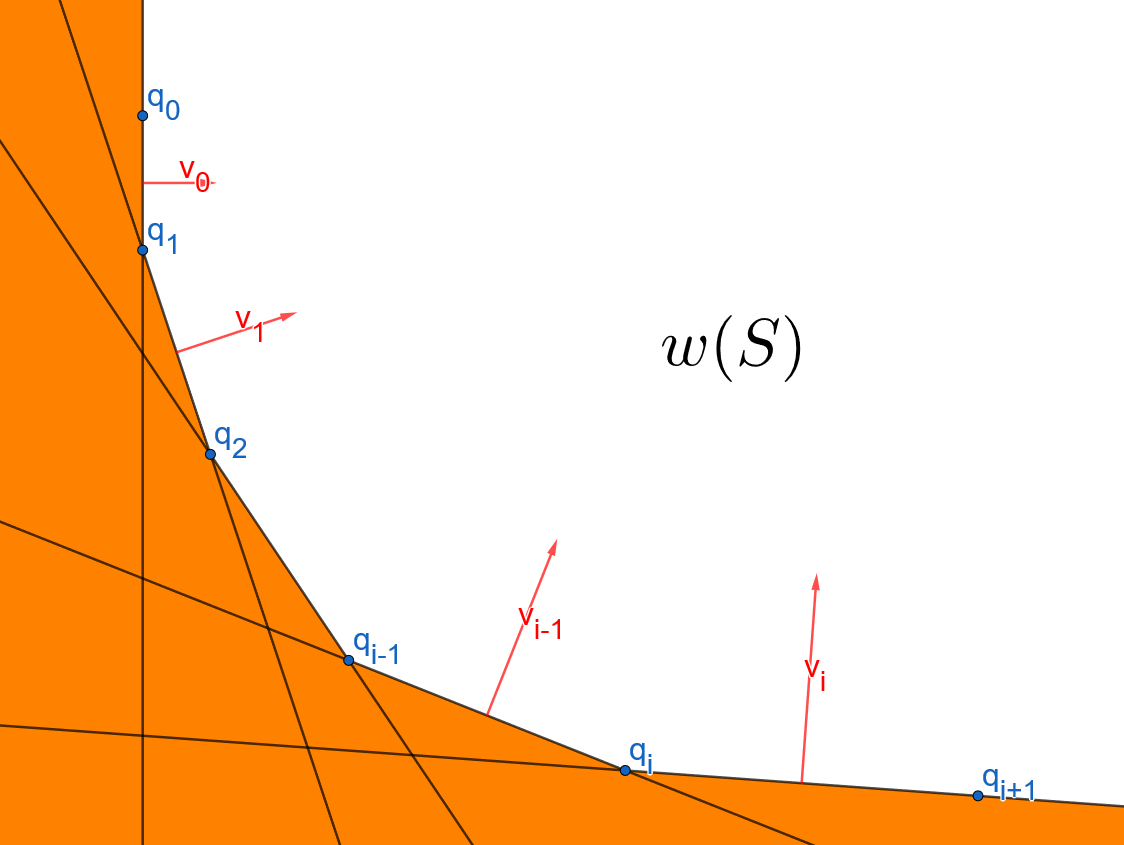
Proof.
As shown in Figure 1, the set of all objective values is contained in the intersection of the upper-half planes of the lines . For any such , let
This vector is normal to the line . Also, lies entirely in one of the half planes delimited by , that is pointing towards. Thus, for all if and only if for any point lying on , with equality if and only if . Now let us fix . We know that lies on both and , so, for all and , with equality if and only if or , respectively. By summing these two inequalities, we get , that is , with equality if and only if . Since and are extremal points, these two lines cannot be parallel, hence , which concludes the proof. ∎
We suppose from now on that the population contains a spanning tree, which is true after an expected number of iterations by Lemmas 8 and 9.
To prove the claimed upper bound, we use multiplicative drift analysis Doerr et al. 2012 on a quantity derived from these functions. A reminder for this technique may be found in appendix of the Arvix version of the paper.
To use the multiplicative drift theorem, we introduce a potential that has a multiplicative drift. For a given population , let
Lemma 14.
Let be the population of the NSGA-II or the GSEMO algorithm after iterations. Then for any , and are nonnegative integers and are non-increasing with respect to t.
Proof.
In order to apply drift analysis, we need another lemma given by Neumann and Wegener 2007.
Lemma 15 (Neumann and Wegener 2007, Lemma 2).
Let be any function which is a linear combination with nonnegative coefficients of and . Let be a search point describing a spanning tree . Let be the minimum value taken by on spanning trees. Then there exists a set of 2-bit flips resulting on new spanning trees, such that the average weight decrease of these flips is at least
We now prove the following lemma.
Lemma 16.
The expected number of generations until the NSGA-II (resp. GSEMO), working on the fitness function with a population of size and with any offspring generation mechanism (resp. its intrinsic mechanism), constructs a population such that is upper bounded by (resp. ).
Proof.
For any and any iteration , let be an individual such that . Then, let be a lower bound over all pairs of bit positions of the probability that there exists, in the offspring, a child generated with as (one of) the parent(s) that differs from on exactly this pair of bits. For the NSGA-II algorithm, by definition of , we have .
For the GSEMO algorithm, if there is at least one spanning tree in the population, the size of the population is upper-bounded by by Lemma 12. Therefore,
We also denote when analysing GSEMO, such that we have for both algorithms.
We now apply drift analysis on . Indeed, for , is a linear combination of and with non-negative coefficients minimum .
Focusing only on the set of 2-bits flips given by Lemma 15 on a search point being one of , and noticing that, since is non-increasing (Lemma 14), all other bit flips contribute positively to the drift, we have
Using this estimate, we show the following lower bound for the drift of our potential.
Let . Since is an non-negative integer, the minimum strictly positive value of is . Since each edge has a weight at most , . Finally, since the convex hull is an incomparable set, we have by Lemma 12. Hence we obtain
Using multiplicative drift theorem, we obtain
We then conclude the proof by plugging in the value of for GSEMO, which does only one fitness evaluation per iteration. ∎
5 Study of Offspring Generation Mechanisms of the NSGA-II
This section is dedicated to demonstrating applications of Theorem 6 on the study of the influence of particular offspring generation mechanisms on the expected runtime of the NSGA-II before finding the extremal points.
We start with a very rudimentary mechanism, composed of fair selection (selecting every individual in as a parent), and standard bitwise mutation with constant , (mutating every bit of a given parent with probability ). Then we can define the lower bounds on the success probabilities as follows.
Theorem 6 then gives the following corollary.
Corollary 17.
The expected time until the NSGA-II, working on the fitness function with a population of size and using standard bitwise mutation and fair selection, constructs a population which includes a spanning tree for each extremal vector of conv() is upper bounded by generations, and
fitness evaluations.
With note that the same result would hold when replacing bitwise mutation with fast mutation Doerr et al. 2017, which proved to be advantageous in some multi-objective problems Doerr and Zheng 2021.
Theorem 6 also ensures that adding crossover with constant probability does not worsen the asymptotic complexity of the NSGA-II. To be more precise, let us consider a random monoparental reproduction scheme , which, from an individual , generates an offspring . From this operator, and a given crossover operator we derive a biparental reproduction scheme , which, from a pair of individuals , generates, with probability , the children and , and with probability , the children , and . Now, consider an offspring generation scheme which puts the selected parents into pairs and applies to these pairs. Finally, note that if , and , are the pairs of probabilities defined in 6 for the offspring generation mechanism using or , then we have trivially and . This gives the following corollary.
Corollary 18.
For a given NSGA-II implementation, replacing by , as described above (i.e. adding crossover with constant probability) does not worsen the asymptotic expected runtime (up to a multiplicative constant).
Finally, to demonstrate the relevance of the parameter, let us introduce a problem-specific “balanced” mutation operator, described in Neumann and Wegener 2007. For any tree individual the mutation operator flips each 1-bit with probability , and each 0-bit with probability , and applies standard bitwise mutation otherwise. We use fair selection for this example. By definition, the value of remains unchanged compared to standard bitwise mutation, that is, . However, one can show that is increased from to (see appendix of the Arvix version of the paper). Theorem 6 automatically gives:
Corollary 19.
The expected runtime of the NSGA-II, working on the fitness function , with , using fair selection and balanced mutation is generations and
fitness evaluations.
6 Conclusion
In this first mathematical runtime analysis of the NSGA-II on a combinatorial optimization problem, we provided a general approach to proving runtime guarantees for MOEAs solving the bi-objective MST problem. For the global SEMO, this gave a bounds lower than the previously known ones by a factor of . More interestingly, we could prove the same performance guarantees for the much more complex NSGA-II. Our result applies to several variants of the NSGA-II, including some that use crossover. As for the simple global SEMO algorithm, we obtain better guarantees when employing a balanced mutation operator (which supports the general belief that analyses on simple toy algorithms can nevertheless give useful hint for the use of more complex algorithms).
Overall, this work indicate that mathematical runtime analyses for the NSGA-II are possible also for combinatorial optimization problems. In this first work, we mostly concentrated on proving performance guarantees at all. For future work, it would be interesting to derive more insights on how to optimally use the NSGA-II on the particular problem (we only saw that balanced mutation is preferable). That such results are possible in principle is again indicated by the simpler works on artificial benchmarks, where, e.g., Doerr and Qu 2023a gave some indications on the right mutation rate. Clearly, runtime analyses of the NSGA-II on other combinatorial optimization problems would also be desirable to put this research direction on a broader basis.
Acknowledgments
This work was supported by a public grant as part of the Investissements d’avenir project, reference ANR-11-LABX-0056-LMH, LabEx LMH and a fellowship via the International Exchange Program of École Polytechnique.
References
- Antipov and Doerr [2021] Denis Antipov and Benjamin Doerr. A tight runtime analysis for the EA. Algorithmica, 83:1054–1095, 2021.
- Arroyo et al. [2008] José Elias Claudio Arroyo, Pedro Sampaio Vieira, and Dalessandro Soares Vianna. A GRASP algorithm for the multi-criteria minimum spanning tree problem. Annals of Operations Research, 159:125–133, 2008.
- Auger and Doerr [2011] Anne Auger and Benjamin Doerr, editors. Theory of Randomized Search Heuristics. World Scientific Publishing, 2011.
- Bäck [1993] Thomas Bäck. Optimal mutation rates in genetic search. In International Conference on Genetic Algorithms, ICGA 1993, pages 2–8. Morgan Kaufmann, 1993.
- Bian and Qian [2022] Chao Bian and Chao Qian. Better running time of the non-dominated sorting genetic algorithm II (NSGA-II) by using stochastic tournament selection. In Parallel Problem Solving From Nature, PPSN 2022, pages 428–441. Springer, 2022.
- Bian et al. [2023] Chao Bian, Yawen Zhou, Miqing Li, and Chao Qian. Stochastic population update can provably be helpful in multi-objective evolutionary algorithms. In International Joint Conference on Artificial Intelligence, IJCAI 2023. ijcai.org, 2023. To appear. Available as arXiv:2306.02611.
- Bossek and Grimme [2017] Jakob Bossek and Christian Grimme. A Pareto-beneficial sub-tree mutation for the multi-criteria minimum spanning tree problem. In Symposium Series on Computational Intelligence, SSCI 2017, pages 1–8. IEEE, 2017.
- Brockhoff et al. [2008] Dimo Brockhoff, Tobias Friedrich, and Frank Neumann. Analyzing hypervolume indicator based algorithms. In Parallel Problem Solving from Nature, PPSN 2008, pages 651–660. Springer, 2008.
- Crawford [2019] Victoria G. Crawford. An efficient evolutionary algorithm for minimum cost submodular cover. In International Joint Conference on Artificial Intelligence, IJCAI 2019, pages 1227–1233. ijcai.org, 2019.
- Dang et al. [2021] Duc-Cuong Dang, Anton V. Eremeev, and Per Kristian Lehre. Escaping local optima with non-elitist evolutionary algorithms. In AAAI Conference on Artificial Intelligence, AAAI 2021, pages 12275–12283. AAAI Press, 2021.
- Dang et al. [2023a] Duc-Cuong Dang, Andre Opris, Bahare Salehi, and Dirk Sudholt. Analysing the robustness of NSGA-II under noise. In Genetic and Evolutionary Computation Conference, GECCO 2023. ACM, 2023. To appear. Available as arXiv:2306.04525.
- Dang et al. [2023b] Duc-Cuong Dang, Andre Opris, Bahare Salehi, and Dirk Sudholt. A proof that using crossover can guarantee exponential speed-ups in evolutionary multi-objective optimisation. In Conference on Artificial Intelligence, AAAI 2023. AAAI Press, 2023. To appear. Available as arXiv:2301.13687.
- Deb et al. [2002] Kalyanmoy Deb, Amrit Pratap, Sameer Agarwal, and T. Meyarivan. A fast and elitist multiobjective genetic algorithm: NSGA-II. IEEE Transactions on Evolutionary Computation, 6:182–197, 2002.
- Doerr and Neumann [2020] Benjamin Doerr and Frank Neumann, editors. Theory of Evolutionary Computation—Recent Developments in Discrete Optimization. Springer, 2020. Also available at http://www.lix.polytechnique.fr/Labo/Benjamin.Doerr/doerr˙neumann˙book.html.
- Doerr and Qu [2023a] Benjamin Doerr and Zhongdi Qu. A first runtime analysis of the NSGA-II on a multimodal problem. Transactions on Evolutionary Computation, 2023. https://doi.org/10.1109/TEVC.2023.3250552.
- Doerr and Qu [2023b] Benjamin Doerr and Zhongdi Qu. From understanding the population dynamics of the NSGA-II to the first proven lower bounds. In Conference on Artificial Intelligence, AAAI 2023. AAAI Press, 2023. To appear. Available as 2209.13974.
- Doerr and Qu [2023c] Benjamin Doerr and Zhongdi Qu. Runtime analysis for the NSGA-II: Provable speed-ups from crossover. In Conference on Artificial Intelligence, AAAI 2023. AAAI Press, 2023. To appear. Available as arXiv:2208.08759.
- Doerr and Zheng [2021] Benjamin Doerr and Weijie Zheng. Theoretical analyses of multi-objective evolutionary algorithms on multi-modal objectives. In Conference on Artificial Intelligence, AAAI 2021, pages 12293–12301. AAAI Press, 2021.
- Doerr et al. [2012] Benjamin Doerr, Daniel Johannsen, and Carola Winzen. Multiplicative drift analysis. Algorithmica, 64:673–697, 2012.
- Doerr et al. [2015] Benjamin Doerr, Carola Doerr, and Franziska Ebel. From black-box complexity to designing new genetic algorithms. Theoretical Computer Science, 567:87–104, 2015.
- Doerr et al. [2016] Benjamin Doerr, Wanru Gao, and Frank Neumann. Runtime analysis of evolutionary diversity maximization for OneMinMax. In Genetic and Evolutionary Computation Conference, GECCO 2016, pages 557–564. ACM, 2016.
- Doerr et al. [2017] Benjamin Doerr, Huu Phuoc Le, Régis Makhmara, and Ta Duy Nguyen. Fast genetic algorithms. In Genetic and Evolutionary Computation Conference, GECCO 2017, pages 777–784. ACM, 2017.
- Doerr et al. [2022] Benjamin Doerr, Omar El Hadri, and Adrien Pinard. The global SEMO algorithm. In Genetic and Evolutionary Computation Conference, GECCO 2022, pages 520–528. ACM, 2022.
- Droste et al. [2002] Stefan Droste, Thomas Jansen, and Ingo Wegener. On the analysis of the (1+1) evolutionary algorithm. Theoretical Computer Science, 276:51–81, 2002.
- Ehrgott [2005] Matthias Ehrgott. Multicriteria Optimization. Springer, 2nd edition, 2005.
- Friedrich et al. [2010] Tobias Friedrich, Jun He, Nils Hebbinghaus, Frank Neumann, and Carsten Witt. Approximating covering problems by randomized search heuristics using multi-objective models. Evolutionary Computation, 18:617–633, 2010.
- Giel [2003] Oliver Giel. Expected runtimes of a simple multi-objective evolutionary algorithm. In Congress on Evolutionary Computation, CEC 2003, pages 1918–1925. IEEE, 2003.
- Hamacher and Ruhe [1994] Horst W. Hamacher and Günther Ruhe. On spanning tree problems with multiple objectives. Annals of Operations Research, 52:209–230, 1994.
- Horoba [2009] Christian Horoba. Analysis of a simple evolutionary algorithm for the multiobjective shortest path problem. In Foundations of Genetic Algorithms, FOGA 2009, pages 113–120. ACM, 2009.
- Huang and Zhou [2020] Zhengxin Huang and Yuren Zhou. Runtime analysis of somatic contiguous hypermutation operators in MOEA/D framework. In Conference on Artificial Intelligence, AAAI 2020, pages 2359–2366. AAAI Press, 2020.
- Huang et al. [2019] Zhengxin Huang, Yuren Zhou, Zefeng Chen, and Xiaoyu He. Running time analysis of MOEA/D with crossover on discrete optimization problem. In Conference on Artificial Intelligence, AAAI 2019, pages 2296–2303. AAAI Press, 2019.
- Jansen et al. [2005] Thomas Jansen, Kenneth A. De Jong, and Ingo Wegener. On the choice of the offspring population size in evolutionary algorithms. Evolutionary Computation, 13:413–440, 2005.
- Jansen [2013] Thomas Jansen. Analyzing Evolutionary Algorithms – The Computer Science Perspective. Springer, 2013.
- Knowles and Corne [2000] Joshua D. Knowles and David Corne. Approximating the nondominated front using the Pareto archived evolution strategy. Evolutionary Computation, 8:149–172, 2000.
- Knowles and Corne [2001] Joshua D. Knowles and David W. Corne. A comparison of encodings and algorithms for multiobjective minimum spanning tree problems. In Congress on Evolutionary Computation, CEC 2001, pages 544–551. IEEE, 2001.
- Lai and Zhou [2020] Xinsheng Lai and Yuren Zhou. Analysis of multiobjective evolutionary algorithms on the biobjective traveling salesman problem (1, 2). Multimedia Tools and Applications, 79:30839–30860, 2020.
- Laumanns et al. [2002] Marco Laumanns, Lothar Thiele, Kalyanmoy Deb, and Eckart Zitzler. Combining convergence and diversity in evolutionary multiobjective optimization. Evolutionary Computation, 10:263–282, 2002.
- Li et al. [2016] Yuan-Long Li, Yu-Ren Zhou, Zhi-Hui Zhan, and Jun Zhang. A primary theoretical study on decomposition-based multiobjective evolutionary algorithms. IEEE Transactions on Evolutionary Computation, 20:563–576, 2016.
- Majumder et al. [2020] Saibal Majumder, Mohuya B. Kar, Samarjit Kar, and Tandra Pal. Uncertain programming models for multi-objective shortest path problem with uncertain parameters. Soft Computing, 24:8975–8996, 2020.
- Mühlenbein [1992] Heinz Mühlenbein. How genetic algorithms really work: mutation and hillclimbing. In Parallel Problem Solving from Nature, PPSN 1992, pages 15–26. Elsevier, 1992.
- Neumann and Theile [2010] Frank Neumann and Madeleine Theile. How crossover speeds up evolutionary algorithms for the multi-criteria all-pairs-shortest-path problem. In Parallel Problem Solving from Nature, PPSN 2010, Part I, pages 667–676. Springer, 2010.
- Neumann and Wegener [2006] Frank Neumann and Ingo Wegener. Minimum spanning trees made easier via multi-objective optimization. Natural Computing, 5:305–319, 2006.
- Neumann and Wegener [2007] Frank Neumann and Ingo Wegener. Randomized local search, evolutionary algorithms, and the minimum spanning tree problem. Theoretical Computer Science, 378:32–40, 2007.
- Neumann and Witt [2010] Frank Neumann and Carsten Witt. Bioinspired Computation in Combinatorial Optimization – Algorithms and Their Computational Complexity. Springer, 2010.
- Neumann and Witt [2022] Frank Neumann and Carsten Witt. Runtime analysis of single- and multi-objective evolutionary algorithms for chance constrained optimization problems with normally distributed random variables. In International Joint Conference on Artificial Intelligence, IJCAI 2022, pages 4800–4806. ijcai.org, 2022.
- Neumann [2007] Frank Neumann. Expected runtimes of a simple evolutionary algorithm for the multi-objective minimum spanning tree problem. European Journal of Operational Research, 181:1620–1629, 2007.
- Nguyen et al. [2015] Anh Quang Nguyen, Andrew M. Sutton, and Frank Neumann. Population size matters: rigorous runtime results for maximizing the hypervolume indicator. Theoretical Computer Science, 561:24–36, 2015.
- Parraga-Alava et al. [2017] Jorge Parraga-Alava, Márcio Dorn, and Mario Inostroza-Ponta. Using local search strategies to improve the performance of NSGA-II for the multi-criteria minimum spanning tree problem. In Congress on Evolutionary Computation, CEC 2017, pages 1119–1126. IEEE, 2017.
- Qian et al. [2019] Chao Qian, Yang Yu, Ke Tang, Xin Yao, and Zhi-Hua Zhou. Maximizing submodular or monotone approximately submodular functions by multi-objective evolutionary algorithms. Artificial Intelligence, 275:279–294, 2019.
- Rudolph [1997] Günter Rudolph. Convergence Properties of Evolutionary Algorithms. Verlag Dr. Kovǎc, 1997.
- Thierens [2003] Dirk Thierens. Convergence time analysis for the multi-objective counting ones problem. In Evolutionary Multi-Criterion Optimization, EMO 2003, pages 355–364. Springer, 2003.
- Wietheger and Doerr [2023] Simon Wietheger and Benjamin Doerr. A mathematical runtime analysis of the Non-dominated Sorting Genetic Algorithm III (NSGA-III). In International Joint Conference on Artificial Intelligence, IJCAI 2023. ijcai.org, 2023. To appear. Available as arXiv:2211.08202.
- Witt [2006] Carsten Witt. Runtime analysis of the ( + 1) EA on simple pseudo-Boolean functions. Evolutionary Computation, 14:65–86, 2006.
- Zheng and Doerr [2022a] Weijie Zheng and Benjamin Doerr. Better approximation guarantees for the NSGA-II by using the current crowding distance. In Genetic and Evolutionary Computation Conference, GECCO 2022, pages 611–619. ACM, 2022.
- Zheng and Doerr [2022b] Weijie Zheng and Benjamin Doerr. Runtime analysis for the NSGA-II: proving, quantifying, and explaining the inefficiency for three or more objectives. CoRR, abs/2211.13084, 2022.
- Zheng et al. [2022] Weijie Zheng, Yufei Liu, and Benjamin Doerr. A first mathematical runtime analysis of the Non-Dominated Sorting Genetic Algorithm II (NSGA-II). In Conference on Artificial Intelligence, AAAI 2022, pages 10408–10416. AAAI Press, 2022.
- Zhou et al. [2011] Aimin Zhou, Bo-Yang Qu, Hui Li, Shi-Zheng Zhao, Ponnuthurai Nagaratnam Suganthan, and Qingfu Zhang. Multiobjective evolutionary algorithms: A survey of the state of the art. Swarm and Evolutionary Computation, 1:32–49, 2011.
- Zhou et al. [2019] Zhi-Hua Zhou, Yang Yu, and Chao Qian. Evolutionary Learning: Advances in Theories and Algorithms. Springer, 2019.
Appendix A Appendix
A.1 Illustration of conv()

A.2 Fast-Non-Dominated-Sort
while do 6
for do 7
if then 9
A.3 Proof of Lemma 8
Proof.
First, we bound the expected time before the population contains a connected graph. Note that the fitness function is constructed in such a way that if are such that , then . Thus, at any time, contains individuals all having the exact same number of components. Moreover, this number is non-increasing. Indeed, if is any individual in at iteration , then any offspring having a bigger number of connected components than would be dominated by , and thus would have rank at least . Now, if at iteration , consists of individuals with connected components, since is connected, there are for each individual at least edges of whose inclusion reduces the number of components. Hence, by definition of the probability that the number of connected components of individuals in decreases at iteration is lower bounded by (Note that the left term is the probability that at least one of the edges is added, but no other). Thus, the expected waiting time for a decrease is at most . Hence, the expected time until the population consists only of connected graphs is upper bounded by
Now, we bound the expected time before the population contains a spanning tree, from the moment it contains a connected graph. From this point, we know that all individuals in are connected graphs. Also, still by construction of the fitness function, consists of individuals having the exact same number of edges, and we prove that this number is still non-increasing using the same argument as for connected components. If consists of non-spanningtree individuals with edges, , then for each individual in , there are exactly edges whose exclusion decreases the number of edges without increasing the number of connected components. Using the same arguments as for connected graphs, we deduce that the expected time until contains spanning trees is at most
We get the claimed upper bound on the whole process simply by summing the two latter.∎
A.4 Proof of Lemma 10
Proof.
Let and be the population sorted of and respectively. If , is at the position and in list and respectively, its crowding distance is positive if and only if one of the 4 following inequalities is true.
- •
- •
- •
- •
However the lists are monotonic, meaning that for a fixed weight value , the indices such that form a contiguous segment of . Hence, only the two border indices of this segment satisfy one of the two conditions on . We deduce that, for a fixed objective value , there are at most individuals such that having positive crowding distance.
Moreover, for a given objective value , there is at least one individual such that with a positive crowding distance. Indeed, since is incomparable, all individuals with have an objective value , so if we denote the smallest index such that in the sorted list, then is an individual satisfying these requirements. Let us now distinguish two cases. Now, let us distinguish two cases.
- •
If , then, every individual in is selected for the next generation and so the lemma holds.
- •
if , first observe that consists only of spanning trees as it contains at least one spanning tree by assumption and a spanning tree dominates every non-spanning tree solution. Moreover, is an incomparable set. Using Lemma 12 it follows that . But we know that for each , there are at most 4 individuals with and . Thus, there are at most individuals in with positive crowding distance. By definition of the NSGA-II algorithm, each individual from with positive crowding distance remains. Since there is at least one individual with positive crowding distance for each objective value, for any objective value , there is an individual in the next iteration such that .
Now observe that for any , for any by definition, there exists an such that . So the individual in the next iteration which has the same objective value as will dominate . This concludes the proof. ∎
A.5 The Multiplicative Drift Theorem
Theorem 20 (Multiplicative Drift Theorem Doerr and Neumann 2020).
Let be a sequence of non-negative random variables with a finite state space such that . Let , let and, for and , define the drift . Suppose there exists such that for all and all the drift is
Then,
A.6 Lower bound for the drift of
We show the following lower bound for the drift of our potential.
Proof.
Let
Then, we have:
A.7 -bound for balanced mutation and fair selection
Let be any tree individual of the first front of any population . Note that since is a tree, it has exactly edges, that is, 1-bits. Let be the positions of a pair of bits of different values. Without loss of generality, we can suppose that the bit at position (respectively ) is a 1 (respectively a 0). Since we are using fair selection, will generate a child with probability . Then, by definition of balanced mutation:
- •
The probability that and differ on bit is
- •
The probability that and differ on bit is
- •
The probability that and are equal on all other bits is
By multiplying these three probabilities, we get the probability that and differ on exactly bits and . Thus we can set
∎