Classification of Orbits in Poincaré Maps using Machine Learning

Chandrika Kamath
Lawrence Livermore National Laboratory 7000 East Avenue, Livermore, CA 94551, USA kamath2@llnl.gov

April 17, 2022

Abstract

Poincaré plots, also called Poincaré maps, are used by plasma physicists to understand the behavior of magnetically confined plasma in numerical simulations of a tokamak. These plots are created by the intersection of field lines with a two-dimensional poloidal plane that is perpendicular to the axis of the torus representing the tokamak. A plot is composed of multiple orbits, each created by a different field line as it goes around the torus. Each orbit can have one of four distinct shapes, or classes, that indicate changes in the topology of the magnetic fields confining the plasma. Given the $(x,y)$ coordinates of the points that form an orbit, the analysis task is to assign a class to the orbit, a task that appears ideally suited for a machine learning approach. In this paper, we describe how we overcame two major challenges in solving this problem - creating a high-quality training set, with few mislabeled orbits, and converting the coordinates of the points into features that are discriminating, despite the variation within the orbits of a class and the apparent similarities between orbits of different classes. Our automated approach is not only more objective and accurate than visual classification, but is also less tedious, making it easier for plasma physicists to analyze the topology of magnetic fields from numerical simulations of the tokamak.

1 Introduction

The quest for low-cost fusion power has led to the construction of experimental devices such as the DIII-D[8], an operational device for conducting magnetic fusion research, and ITER [16], an international project to help make the transition from studies of plasma physics to electricity-generating fusion power plants. These devices, called tokamaks, use magnetic fields to confine the fusion fuel in the form of a plasma, enabling physicists to perform experiments to determine the best shape for the hot reacting plasma and the magnetic fields necessary to hold it in place. To complement the experiments, computer simulations are used to gain an understanding of the complex physics of the plasmas, design new reactors, and select the parameters to be used in experiments. Data from both the experiments and the simulations are analyzed to provide the insights that will contribute to achieving the goal of fusion power.

Refer to caption — Figure 1: (a) Schematic view of a tokamak, in the form of a torus, showing the generation of the Poincare plot. Six poloidal planes are shown as ellipses. An orbit, shown as points on the grey ellipse, is formed by the intersections of a field line with the ellipse as the line is traced around the torus. (b) A collection of orbits in a poloidal plane. The magnetic axis is indicated by a red cross.


(a)	(b)	(c)	(d)

Figure 2: Sample orbits illustrating the four classes - (a) a quasiperiodic orbit; (b) a separatrix orbit with three lobes, where a lobe is the region between the ’X’-points where the two curves of the separatrix cross; (c) an island orbit with five islands; and (d) a stochastic orbit. The number of points in the orbits range from 4000 to 8000.

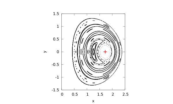
In this paper, we focus on a specific analysis problem that arises in both simulation and experimental data, namely, the classification of orbits in a Poincaré map, also called a Poincaré plot. These two-dimensional plots are obtained for planes, called poloidal planes, which intersect the torus-shaped tokamak perpendicular to the magnetic axis, as shown in Figure 1(a). A plot consists of several orbits, each composed of a number of points (Figure 1(b)). For a given orbit, these points are the intersections of a field line (the solid lines in Figure 1(a)) with a poloidal plane, as the field line is followed around the torus. There are four distinct shapes traced out by these points, leading to four classes of orbits: quasi-periodic, separatrix, island chain, and stochastic, as shown in Figure 2. In some cases, the orbit shows its distinctive shape with just a few points, corresponding to the first few intersections of the field line with the poloidal plane. In other cases, an orbit may appear to be of one class, say island chain, initially, but become a separatrix as additional points are added to the orbit. When the data are generated by a computer simulation, floating point errors can build up as the field lines are traced around the torus, resulting in noise in the location of the later points.

These Poincaré plots provide a convenient way to diagnose, at a glance, changes in the topology of the magnetic fields confining the plasma over time. The goal is to avoid undesirable changes that would result in the hot core of the plasma escaping to mix with the cooler outer regions. Whether the hot plasma is confined or not is reflected in the shape of the orbits: quasi-periodic orbits are indicative of nested magnetic surfaces which provide good confinement; a separatrix indicates reconnection, or rapid changes in the topology; while islands and stochastic regions indicate progressively worse confinement.

Classifying the orbits visually can be tedious, error-prone, and subjective. When the number of orbits is large, as a result of many simulations run over many time steps, it becomes clear that there is a need for an automated approach. An obvious solution is to create a training set by extracting features representing each orbit, followed by a machine learning classifier for prediction. However, the implementation of this solution is not straight-forward due to challenges in labeling the orbits and in identifying relevant features for orbits of different classes (Section 2). In this paper, we describe how we address these challenges (Section 4), and discuss the results of our experiments with i) decision trees for predicting the class of an orbit, and ii) feature selection for understanding which features are more relevant in discriminating among the classes (Section 5). We conclude the paper with a summary of our work in Section 6.

Our contributions in this paper are as follows: given this rather unusual data set, where an instance, or orbit, is a collection of points in two-dimensions, we show how we can transform the $(x,y)$ coordinates of the points into a representation of the visual structure of the orbit. Using simple, but interpretable, classifiers, we show how we can generate a high-quality training data set by refining both the assignment of correct class labels to the orbits and the representative features extracted for each orbit. This approach allows us to capture the subtle differences between orbits of different classes that appear similar when viewed as a whole, as well as the similarities within orbits of a class despite the variation in their shape. As a result, we achieve higher accuracy than that obtained using visual classification. By automating the step of classification of the orbits in a Poincaré plot, we provide plasma physicists improved capability to understand their simulations.

2 Challenges to the analysis

At first glance, this problem of classification of the orbits appears relatively straightforward, and one that can be solved easily as the four orbits shown in Figure 2 have distinctive characteristics. The quasiperiodic orbit appears as points on a single closed curve; the separatrix appears as two intertwined curves; the island chain has angular gaps; and there is no structure to the points in a stochastic orbit. Therefore, by assigning a class label to each orbit and representing it with a suitable set of features, we can create a training data set that we could use to build a machine learning model for classification of orbits. However, a closer inspection of the data indicates two main challenges, which we discuss in detail next.

2.1 Generating a correctly-labeled training set

To generate the training set, we started by visually assigning one of the four class labels to each orbit. Further, since we had a limited set of orbits (four sets of 66 orbits each), many with several thousands of points, we could create a series of orbits from each orbit by using only the initial intersections of the field line with the poloidal plane. Thus, if an orbit of a specific class was defined by $m$ points, $m>1000$ , we created separate derived orbits by using the first $1000,1500,2000,...$ points and assigned them the same class.

However, we then realized that the class of the derived orbits could vary as the number of points was increased. For example, in Figure 3 panel (a), an orbit appears as a quasiperiodic when we plot the first 500 points. At 1000 points, we see a handful of points forming an inner curve, points that could be easily overlooked in a visual labeling of the orbit. This inner curve takes shape only when many more points are added, clearly indicating a separatrix orbit in panels (c) and (d). A similar example is shown in Figure 4, where the class of the orbit changes from island chain to separatrix to mildly stochastic as the number of points in the orbit is increased. This meant that we needed to visually inspect each of the derived orbits to assign a class label; we could not simply assign them to the same class.


(a)	(b)	(c)	(d)

Figure 3: Views of a separatrix orbit as the number of points is increased from (a) 500, showing a quasiperiodic to (b) 1000 points, which is a separatrix with the inner curve made up of very few points, to a clear separatrix at (c) 2000 and finally, (d) 4860 points.



(a)	(b)	(c)	(d)

Figure 4: A separatrix orbit is shown using the first (a) 500; (b) 2000; (c) 3000; and (d) 5000 points, with the bottom row showing the details of the left part of the orbit. The orbits have a multi-scale structure, as they appear to be quasiperiodic at a coarse scale (top row), but the fine scale detail indicates that as the number of points is increased, the class changes from island chain, to separatrix, to mildly stochastic.

We observed that some orbits, especially the separatrix, have some stochasticity, especially for a large number of points. This results from the way in which the field lines are traced along the torus. A true stochastic orbit has the points spread out over a large radial distance as in Figure 2(d).

Figure 4 also illustrates the second challenge in labeling orbits — this orbit, regardless of the number of points, appears to be quasiperiodic when viewed as a whole; we need to look at the detail to determine the correct class. Figure 5 shows other examples where a visual inspection of the full orbit is insufficient to assign the correct class label. Panel (a) appears to be a single island in the form of a crescent, but is actually an island composed of thin islands, that is, the crescent shape will always be composed of incomplete segments. In panels (b) and (c), we see that, what appear to be a quasiperiodic orbit and an incomplete quasiperiodic orbit, are actually a separatrix and an island chain, respectively, where the lobes of the separatrix and the islands are very thin, with a very small radial variation. Based on this example, the orbit in Figure 6(a) could be either an incomplete quasiperiodic or an island chain; as more points are added, it could be a quasiperiodic or a very thin separatrix. The details in the bottom row correctly classify this orbit as quasiperiodic, with a very small amount of stochasticity when the number of points is large.



(a)	(b)	(c)

Figure 5: Thin island chains and narrow separatrix orbits can be difficult to classify visually. The details of the region on the left of each orbit (shown in the bottom row) help in classification. (a) A single island in the form of a crescent is found to be composed of several segments that are islands themselves. (b) A very thin separatrix that appears to be a quasiperiodic orbit. (c) An island chain with seven islands that appears as an incomplete quasiperiodic orbit.



(a)	(b)	(c)

Figure 6: A quasiperiodic that could be a thin island chain at 500 points (a) is confirmed to be a quasiperiodic when more points are added in (b) and (c) and a detailed view is observed (bottom row). The detailed view in (c) appears to indicate a stochastic orbit, but the radial range of values is very small, unlike a stochastic orbit.

This multi-scale nature of some of the orbits, where an orbit appears to be of one class when viewed at a coarse scale, but is of a different class when viewed at a finer scale (that is, a zoomed-in view), further makes it challenging to label the orbits correctly. We can no longer rely solely on a visual inspection of the entire orbit to assign a class; requiring a closer inspection of the points makes the class assignment even more tedious. This provides a strong motivation for our work and, as we show later in Section 4.1, we can use the process of automating the assignment of labels to bootstrap the correct assignment of class labels.

2.2 Generating the features for the training set

The second challenging aspect of the problem of orbit classification is the identification and extraction of representative features for each orbit. Obviously, the features selected must be discriminating so they can be used to differentiate among the orbits of different classes. However, as we have seen, the orbits within a class can appear quite different, while orbits from different classes may appear very similar. As a result, obvious features, such as the angular gaps that characterize the island orbits, are not sufficient to differentiate them from incomplete quasiperiodic orbits, while a small radial variation of the points within a small angular window could indicate a quasiperiodic, a thin island chain, or a thin separatrix. There are also other considerations that influence the definition and extraction of representative features:

•

The data are available as $(x,y)$ coordinates of the points in an orbit and must be converted to represent the structure we see when we visualize the orbit, either as a whole, or a zoomed-in view.
•

These features must be invariant to scale, rotation, and translation, as the class of the orbit does not change if it is scaled, rotated, or translated.
•

The features must be robust to noise as small changes in the coordinates of the points in an orbit do not change the orbit class.
•

The features must not depend on the number of points in the orbit, or how far out the orbit is relative to the magnetic axis.

Transforming the $(x,y)$ coordinates of an orbit into a representation of the visual structure we see is what makes this problem unusual and challenging.

3 Related work

We next briefly review existing work related to the classification of orbits in Poincaré maps to place our work in context. The topic of Poincaré plots, or Poincaré maps, is of interest to several communities, including plasma physics [15] and spacecraft trajectory design [18]. A common theme in these classical physics systems, where the dynamics is described in terms of Hamilton’s equations, is identifying regular and chaotic regions in phase space. This specific problem has been addressed using box counting to determine the fractal dimension of a set of points [1] and by calculating the spectrum of Lyapunov exponents using fast algorithms, such as the structure-preserving Gaussian process surrogate [13].

The analysis of Poincaré maps in magnetic confinement fusion, where they are referred to as puncture plots, has been driven by two class of methods. The visualization community has focused on topology-based methods. For example, Sanderson et al. [14] have used field lines with near minimal lengths to determine the topology of a magnetic field, while Tricoche, Garth, and Sanderson [17] have combined a six-stage topological approach, specifically tailored to the data, with visualization of scalar maps to provide context to the topological visualization. These analyses have also included island chain and separatrix orbits, in addition to quasiperiodic and chaotic orbits.

In contrast, the data mining community has taken a feature-based approach. Yip [19] represented an orbit as a minimal spanning tree, a tree that contains all nodes of the graph where the sum of the edge lengths is minimal. Next, edge lengths greater than a specified threshold were removed, splitting the tree into distinct subgraphs, and features were obtained for the full tree and the subgraphs. For example, the diameter of a graph, which is the longest shortest path between any two nodes in the graph was identified, followed by the “branches” of the graph that have only one node in the diameter. Then, each branch was assigned properties, such as a shallow or a deep branch based on its length. The entire orbit was represented by features such as the number of subgraphs and the fraction of nodes that are on a shallow branch. These features were then used in rules to identify the class of an orbit.

In our previous work [2, 3], we started by applying the rule-based approach of Yip to our data sets. We found that we could improve the results by including additional features and by using standard machine learning classifiers instead of a rule based system. While we obtained nearly 90% accuracy rate for classification, our approach was not robust enough to be applied in practice. We found that an orbit had to be represented by a large number of points (2000-2500) for accurate classification and it was challenging to set the values of the many thresholds used in defining the features. In addition, the graph structure was difficult to implement in software, depended on the number of points in an orbit, and was prone to giving incorrect results if any of the key points determining the structure were perturbed slightly. This present work is an attempt to address these deficiencies.

4 Solution Approach

We used a three-step, machine-learning approach to classifying the orbits, starting with the labeling of the orbits and the generation of features for each orbit to create a training data set, followed by building a classification model with the training set to discriminate among the different classes. We used decision trees as our model of choice as it allows us to understand how the decision to assign a specific class is made, allowing us to iteratively refine both the labels assigned to an orbit, as well as the features used to describe it, thus enabling the creation of a high-quality training data set.

4.1 Labeling the orbits

We started by labeling the orbits using a visual inspection to assign each orbit to one of four classes — quasi-periodic, separatrix, island chain, and stochastic. As discussed earlier, given the limited number of orbits, we increased the number of instances in our data set by creating derived orbits composed of the first $k$ points in an orbit, with $k=1000,1500,\ldots$ . The lower bound on $k$ was chosen as we required a certain minimum number of points in an orbit to extract meaningful features. As the class of an orbit can change with increasing number of points, the use of these derived orbits also allows us to increase the diversity of the instances in the training data set.

Initially, we assigned to each derived orbit, the same class as the original orbit, which was determined using a visual inspection of all points at coarse-scale. Next, we created an initial training data set by extracting obvious features for the orbits, such as angular gaps or the radial spread of points, and built a decision tree model. We then found that we needed to improve the robustness of the features extracted as detailed in Section 4.2.3. As we iteratively improved the quality of the features, the prediction error reduced.

We then reached a point where we were unable to reduce the prediction error any further. A closer look at the decision tree model indicated that it would often incorrectly predict quasiperiodic orbits with gaps as island chains, or ones without gaps as separatrix orbits. When we followed the path the features for these orbits took through the decision tree, we found that at the leaf node, all training instances were of the same class as the one predicted for the orbit. This indicated that in the feature space, the orbit being labeled was in a region where the class was different from the class we had assigned. We next checked the features for the orbit to determine whether we had extracted them correctly. In the process, we inspected each orbit closely, and realized that the features extracted were correct, but, as described in Section 2.1, either the orbits had a multiscale nature and we had assigned them to the wrong class, or that the class of the derived orbit, with fewer points, was different from that of the orbit with all the points.

This accidental discovery indicated that we needed to look closely at the details of each orbit to assign the correct class, making the labeling even more tedious. Instead, we used the decision tree model to our advantage and checked the details only for the orbits with incorrect predictions to determine whether we should change the label assigned. This approach reduced some of the tediousness of labeling the orbits and allowed us to bootstrap our way to a higher quality training data set.

4.2 Feature Extraction

The identification and extraction of discriminating features was performed iteratively - we selected a few sample orbits from each class, extracted a set of features and analyzed them to determine if they were representative enough to account for the variation we saw among the orbits. As the quality of the features improved, we used them to build a decision tree classifier and evaluated its accuracy. If certain types of orbits were consistently mis-classified by the model, we followed the features for such orbits through the decision tree, identified the aspect of the orbit that was missing in the existing features, and refined the features, continuing the process until sufficient accuracy was obtained.

The feature extraction consists of three phases - the initial preprocessing of the data, the extraction of local features representing the local region around the points, and the calculation of global features representing the orbit as a whole. We next discuss these phases in detail.

4.2.1 Preprocessing the data

It is possible to use the original $(x,y)$ coordinates of the points that form an orbit to extract the features. However, we found that converting the data to polar coordinates, using the magnetic axis as the origin, exaggerated the radial variation in an orbit, making it easier to differentiate among the orbits. For example, Figure 7, using $(r,\theta)$ coordinates, clearly shows the difference between the quasiperiodic orbit from Figure 2(a) and the very thin separatrix orbit from Figure 5(b).




(a)	(b)	(c)

Figure 7: The orbits in polar coordinates, with the angle,

\theta

, on the

x

-axis and the radius,

r

, on the

y

-axis. (a) The quasiperiodic orbit from Figure 2(a); (b) the island chain orbit from Figure 2(c); and (c) the separatrix orbit from Figure 5(b). Top row:

(x,y)

coordinates, middle row:

(r,\theta)

coordinates, and bottom row: a zoomed-in view of the polar coordinates that highlights the difference between the quasiperiodic and thin separatrix orbits.

4.2.2 Initial extraction of local features

Once we converted the data into polar coordinates, we wanted to extract local features for the orbit, that is, features that represent the structure of the points in a small $\theta$ window. We started by defining these windows based on the $\theta$ value of the points in an orbit. If we created $n$ windows, each subtending an angle $\delta_{n}=360^{\circ}/n$ or $\delta_{n}=2\pi/n$ radians at the magnetic axis, the points in the $i$ -th window would satisfy

-\pi+(i-1)\delta_{n}\leq\theta<-\pi+i\delta_{n}.

(1)

Each point was assigned to one and only one window and all orbits have the same number of windows, $n$ .

Next, for the points in each window, we obtained $r_{max}$ and $r_{min}$ , which are the largest and smallest values of $r$ , respectively, and calculated ${\Delta r}_{max}=\max(r_{max}-r_{min})$ , which is the largest radial width across all windows. The points in each window were then shifted radially by $r_{min}$ so that the minimum $r$ in each window became zero, and scaled by ${\Delta r}_{max}$ , so that the new largest radial width across all the windows in an orbit became 1.0. This scaling normalizes the radial variation in the points within the windows across all orbits, so that separatrix and island orbits with wide lobes are treated similar to those with thin lobes.

After the normalization, we extracted local features for each window, such as the variation in the $r$ values of the points in a window so we could distinguish quasiperiodic orbits from separatrix orbits, as well as island orbits from quasiperiodic orbits with gaps. We also included a simple count of the points in a window, to reflect the observation that the X points of the separatrix and the end regions of islands have a higher concentration of points. These local features for each of the $n$ windows were converted to features for the entire orbit by taking the mean, minimum, and maximum values of the features across the windows. We also included global features, such as the number of windows with no points.

However, our early experiments indicated two problems with this approach to extracting representative features. The first was the definition of a window. The features extracted were very dependent on the angular width of the window, $\delta_{n}$ , and the location of the points in an orbit relative to the boundaries between the windows. This meant that the features were not rotation invariant, as a feature, such as the maximum density of points across all the windows, could vary substantially if we just rotated the orbit.

Figure 8: A subset of the orbits in polar coordinates, with

\theta

on the x-axis and

r

on the y-axis. Top: a separatrix orbit; bottom: a quasiperiodic orbit. The change in

r

over a

3^{\circ}

window centered at -2.2 for the separatrix (in black) is similar to the change in

r

over a

3^{\circ}

window centered at -1.6 for the quasiperiodic orbit (in red). Thus, using the range of

r

values in a window does not indicate whether the points in the window can be fit by one curve or two.

The second issue was that using just the range of $r$ values within a window was not sufficient to determine if the points in a window lay on one curve, as in a quasiperiodic orbit, or two, as in a separatrix or island chain orbits. As shown in Figure 8, when we consider the variation in $r$ in a $3^{\circ}$ window, we can get similar results for a separatrix (top curve, window centered at $\theta=-2.2$ radians) as we would for a quasiperiodic orbit (bottom curve, window centered at $\theta=-1.6$ radians). This holds whether we considered the difference between the largest and smallest $r$ for the points in the window, that is, $|r_{max}-r_{min}|$ , or the maximum difference between $r$ values of consecutive points, that is, $\max_{j}|r_{j}-r_{j+1}|$ .

4.2.3 Robust extraction of local features

These observations prompted us to consider more robust ways to extract local features. To make the features rotation invariant, we re-defined a window to be centered around each of the $m$ points in an orbit, as shown in Figure 9. Thus, instead of a fixed number, $n$ , of non-overlapping windows for all orbits, we now had a variable number, $m$ , of overlapping windows, each centered at a point and subtending an angle of $\delta$ , which we set to $2^{\circ}$ . We continued to use the normalization of the $r$ values as explained earlier so the features are not influenced by the distance of the orbit from the magnetic axis or the width of island and separatrix lobes.

Figure 9: A zoomed in view of a separatrix orbit showing a window centered at the point with

\theta=1.75115

, indicated by the middle vertical line. The two vertical lines on either side indicate the boundaries of a window which is

2^{\circ}=

0.0349 radians wide. All points in this window are used to generate the features associated with the central point.

Next, to determine if the points in a window lay on one curve (as in the case of quasiperiodic orbits) or two curves (as would be the case for island and separatrix orbits), we obtained a least squares fit of a second order polynomial to the points in a window and calculated the maximum error across all points in this window; we refer to this maximum error as lserr, or the least square error for the window. This error is small for quasiperiodic orbits, but large for the other classes, especially for windows where is a radial spread in the spatial distribution of the points.

As the least squares fit, and other features explained next, require a certain minimum number of points within a window, we only consider windows with greater than four points in the rest of the discussion. The points associated with such windows are referred to as valid points.

Next, we required a feature that would represent the spatial distribution of points within each window to help differentiate the random scattering of the points in a stochastic orbit from the more organized distribution of points on two curves seen in the island chain and separatrix orbits. We considered a feature derived from quadrat counts in spatial statistics[7]. A quadrat method essentially divides a region into non-overlapping subsets, often rectangular in shape and then counts the number of points in each subset. These counts can then be used to determine if there is any spatial pattern in the data. A completely random spatial pattern will have a Poisson distribution and can be identified using the property that its mean is equal to its variance. In our problem, we used a $4\times 4$ grid in $(r,\theta)$ over each window, and since we have relatively few points in each window, we used the number of non-zero cells in the grid to represent the “spread” of the points. We expected that if a window has a larger spread, it will have a more stochastic distribution of points.

We calculated two additional features to represent the distribution of points across the orbit. The first was, conc, the concentration of points for each valid window, defined as the number of points in the window, scaled by the number of points in the orbit, so orbits with larger number of points do not result in biased features. The second feature was the difference in the $\theta$ values between a point and the point to its left, which we refer to as ldtheta. Note that we need to consider all points for ldtheta, not just the valid points (that is, those with more than four points in the window) because points with large ldtheta are often in windows with few points.

4.2.4 Calculation of derived features

Thus far, we have considered an angular window in $\theta$ around each point in the orbit and calculated quantities that characterize the distribution of the points in the window. These local features are calculated for windows with more than 4 points and, for each such window, include lserr, which is the maximum error in fitting a second order polynomial to the points; the spread of the points based on quadrat counts; and conc, the concentration of points in the window, which is the scaled number of points. In addition, the feature ldtheta at each point represented angular gaps in the orbit.

These vector-valued, local features describe the region around each valid point. To derive global features, in the form of scalars, that can represent the orbit as a whole, we calculated the mean, maximum, minimum, and standard deviation of the local features across all the valid windows in an orbit. In addition, for ldtheta, we defined a new binary feature, ldtheta_large that was set to 1 if an orbit had any value of ldtheta greater than $10^{\circ}$ , and 0 otherwise.

However, we found that these global quantities did not capture the subtle variations among the orbit classes, such as changes in the local features as we traversed along the orbit or any patterns when two of the local features were considered together. For example, a closer look at the separatrix orbits indicated that the conc value in windows near an X point is higher than in windows near the middle of a lobe, while the lserr value is higher near the middle of the lobe and tapers off near the X points. A similar behavior is seen between the center and the two corners of each island in an island chain.

This observation prompted us to consider the lserr and conc features at each window together. Figure 10, top row, shows the sample orbit of each class from Figure 2. The second row shows the values of lserr and conc features, in red and black, respectively, where the x axis indicates all the valid points in the orbit, going counter clockwise from $-\pi$ to $\pi$ radians. The plots in the second row indicate that the values of lserr for the quasiperiodic orbit are much smaller than for the other three orbits, which is expected. Also, as expected, we see clear peaks and valleys in lserr and conc for the island chain and separatrix orbits, though surprisingly, similar peaks and valleys are also present for the quasiperiodic and stochastic orbits.

Figure 10, third row shows the lserr and conc features after both have been scaled to lie between [0,1] and after minimal smoothing with a mean filter of width 3. We make two main observations on these plots. First, the number of peaks is equal to the number of lobes in the separatrix or the number of islands in the island chain, but, for the quasiperiodic and stochastic orbits, it is not possible to relate the number of peaks to any structures in the orbits. Second, there is a clear pattern in the locations of the peaks and valleys for lserr and conc. Stochastic orbits have the peaks and valleys of the two curves aligned, both in magnitude and location. In island chain, the peaks and valleys are of different magnitude, with the peak of one aligned with the valley of the other, and vice versa. For the separatrix orbit, the magnitudes of the two features are different, with the valleys in lserr aligned with the peaks in conc. In the quasiperiodic orbit, the two features have similar magnitudes and their peaks and valleys are aligned, with the latter more so than the former.

Figure 10: The lserr and conc features, in red and black, respectively, for the four sample orbits from Figure 2. Top row: original orbits, from left to right: quasiperiodic, separatrix, island chain, and stochastic. Second row: the lserr and conc features in the window around each valid point. Third row: the features scaled to [0,1] and smoothed using a simple mean filter of width 3. Fourth row: Smoothed features obtained after decimated wavelet transform until the number of points in an orbit is between 250 and 500. Fifth row: the features after additional smoothing with the decimated wavelet transform until fewer than 100 points are left in the orbit. Rows four and five are referred to as the fine and coarse versions of the two features after wavelet smoothing. Last row: value of the ldtheta variable. The points in rows two to six are ordered by value of

\theta

, going counterclockwise from

-\pi

\pi

radians.

To translate these observations into scalar features we wanted to identify the peaks and valleys in lserr and conc and evaluate their alignment. However, both curves are quite noisy and the minimal smoothing used was insufficient. To further reduce the high frequency components, we applied wavelet smoothing with the biorth 3,1 wavelet [5, 10], as it is a symmetric wavelet with a small support. However, we could not use a fixed number of wavelet levels to apply to each orbit as the length of the two curves varies across orbits. Instead, we applied the decimated wavelet transform until the number of points in the smooth, low-frequency part of the data was in the range [250,500) (for the fine level), and less than 100 (for the coarse level), as shown in Figure 10, third and fourth rows, respectively. We chose two levels to identify the peak-valley alignment in lserr and conc in case the fine level still had some remaining noise, as seen in some of the orbits.

Finally, the last row in Figure 10 shows the values of ldtheta for each of the orbits - note the high peaks for the island chain that are large enough to completely dwarf the values in between the peaks. We used these plots to select the threshold for the ldtheta_large feature.

Next, we used a simple peak finder, and its converse as a valley finder, to identify the peaks and valleys in the coarse and fine resolutions of the two vectors. At each resolution, given the total number of peaks and valleys in lserr (or conc), we identified the fraction of the peaks and valleys of lserr aligned with the peaks and valleys, respectively, of conc, and the fraction that were misaligned, that is, the peaks/valleys of lserr were aligned with the valleys/peaks of conc. These features allowed us to represent the behavior we see in Figure 10. In addition, to account for cases where the peak and valley locations could be off by a small amount, we also calculated an additional feature, the sign alignment; this is the fraction of points where the sign of $\Delta$ lserr and $\Delta$ conc is the same, that is, where lserr and conc are both increasing or both decreasing. This fraction would be large in orbits where the peaks and valleys in the two vectors are aligned.

Table 1 lists the 17 features that represent each orbit; the first three (file name, total number of points in orbit, and the number of points used in the instance) are not used in classification but help to identify the provenance of an orbit. The remaining features were selected after initial experiments with ensembles of decision trees to remove features that were not discriminating. For example, features related to conc, such as its minimum, maximum, and mean across the windows, did not convey any information about the class of an orbit, but the vector of conc values was useful when combined with the lserr vector to identify the relationship of peaks and valleys between the two variables.

Feature name	Description
f0	Orbit file name
f1	Total number of points in orbit
f2	Number of points used in this instance
f3	Maximum lserr, across windows, from polynomial fit in each window
f4	Minimum lserr, across windows, from polynomial fit in each window
f5	Mean lserr, across windows, from polynomial fit in each window
f6	Standard deviation of lserr, across windows, from polynomial fit in each window
f7	Mean spread, across windows
f8	Maximum spread, across windows
f9	Minimum spread, across windows
f10	Fraction of peaks and valleys aligned at fine scale
f11	Fraction of peaks and valleys misaligned at fine scale
f12	Fraction of valid points with sign alignment of $\delta$ lserr and $\delta$ conc at fine scale
f13	Fraction of peaks and valleys aligned at coarse scale
f14	Fraction of peaks and valleys misaligned at coarse scale
f15	Fraction of valid points with sign alignment of $\delta$ lserr and $\delta$ conc at coarse scale
f16	Any points where ldtheta is greater than 10 degrees (Boolean variable)

Table 1: A description of the features extracted for the orbits. The first three features are for identifying the provenance of each orbit and are not used in the classification.

4.3 Feature Selection

Once we have identified and extracted the features for each orbit, it can be helpful to determine if some features are more important than others in classifying the orbits into the four classes. We considered three feature selection methods, described in detail in [6], and summarized briefly as follows:

•

Distance filter: Intuitively, a more discriminating feature will have greater distance between the histograms of the different classes. For each feature, we create a histogram of the values of the feature for each of the four classes and obtain the the Kullback-Leibler (KL) distance between these histograms. The features are ranked by sorting them in descending order of the distances.
•

Chi-square filter: This method ranks features by sorting them in descending order of Chi-square statistics computed from their contingency tables [9]. As our features are all numeric (except for f16), they are first discretized using histograms, before the Chi-square statistic for each feature is calculated.
•

Stump filter: A simple approach to ranking features by importance is to use the split criterion in decision trees that determine which feature to split on at any node of the tree. We consider just the root node (hence the name of this method), where the entire training data set is used. In our work, we use the Gini index [4] and rank the features according to the purity of their optimal split.

4.4 Classification

We have many options for a classifier to use for predicting the class of an orbit. We selected decision trees mainly because they allowed us to understand how decisions were made in assigning the class to an orbit, helping us to improve iteratively, the correctness of class labels and the features extracted for each orbit. The specific algorithm we used was ASPEN, a method to generate an ensemble of trees based on approximate splits [11]. We introduce randomization at each node of the tree in two ways - first, by randomly sampling the instances at a node and selecting a fraction (we use 0.7) for further consideration, and second, by replacing the sorting of feature values by a histogram. At each node, we create a histogram of feature values for the sampled instances, evaluate the splitting criterion at the mid-point of each bin of the histogram, identify the best bin, and then select the split point randomly in this bin. The use of the histograms and the smaller number of samples speeds up the creation of each tree in the ensemble. We use two different splitting criteria - Gini [4] and InfoGain [12] for comparison.

5 Experimental Results and Discussion

We next present the results of feature selection and classification for the features listed in Table 1. We started with 264 orbits, and after removing the orbits with too few points, we split them into individual orbits comprised of the first $1000,1500,\ldots$ points. This resulted in a training set of 1884 instances, each represent by 14 features, f3 through f16, listed in Table 1.

First, Table 2 lists the features in descending order of importance as identified by the three feature selection methods when applied to the full data set. Figure 11 shows how the error rate for five runs of five-fold cross validation varies when we use only the first $k$ features in order of importance. The error rate is for eleven trees using the Gini split criterion and the ensemble approach described in Section 4.4.

Rank order	Distance filter	Chi-square filter	Stump filter
1	f3	f8	f16
2	f8	f7	f3
3	f5	f3	f8
4	f6	f5	f5
5	f7	f6	f6
6	f16	f16	f7
7	f15	f15	f4
8	f4	f4	f14
9	f12	f14	f15
10	f10	f12	f9
11	f14	f10	f12
12	f11	f13	f10
13	f13	f11	f13
14	f9	f9	f11

Table 2: Ordering, by importance, of the 14 features representing the orbits, using three different feature selection methods. Note that the first six features identified by all three methods are the same, and based on Figure 11 reduce the error rate to

\approx

5%.

These results indicate that all three feature selection methods select the same top six features as important, though the order changes with the method as each uses a different metric to evaluate the importance. Figure 11 indicates that when these top six features are considered, the error rate drops to 5%, and stabilizes thereafter. These six features are ldtheta_large, the mean and maximum spread across windows, and the maximum, mean, and standard deviation of lserr, taken across windows, where lserr for a window is the maximum error from a polynomial fit in that window. Interestingly, the peak-valley features are ranked lower in importance; this is likely because features indicating the angular gaps, the radial spread, and the number of curves (one or two) in each window, are more discriminating when the full data set is considered as is the case in the feature selection methods.

Figure 11: Error rate from five runs of five-fold cross validation for the top

k

features identified as important by each of the three feature selection methods. The error stabilizes at 6-7 features. The Gini split criterion is used with eleven trees in the ensemble.

	5 trees	11 trees	21 trees
Gini	4.55 (0.05)	4.02 (0.13)	3.98 (0.07)
InfoGain	3.89 (0.08)	3.60 (0.15)	3.46 (0.13)

Table 3: Error rate for five runs of five-fold cross-validation using Gini and InfoGain split criteria. The values in parenthesis are the standard error across the five folds.

		Predicted Classes
		Q S I R
Actual Classes	Q	757	15	3	3
	S	28	212	2	8
	I	6	2	432	0
	R	2	6	6	402

(a) Five trees, Gini criterion, 4.3% error.

		Predicted Classes
		Q S I R
Actual Classes	Q	762	8	3	5
	S	18	221	2	9
	I	4	3	433	0
	R	0	6	6	404

(b) Five trees, InfoGain criterion, 3.4% error.

		Predicted Classes
		Q S I R
Actual Classes	Q	762	12	2	2
	S	21	220	2	7
	I	6	2	432	0
	R	0	6	6	404

		Predicted Classes
		Q S I R
Actual Classes	Q	763	9	3	3
	S	19	220	2	9
	I	4	2	434	0
	R	0	8	6	402

(d) Eleven trees, InfoGain criterion, 3.45% error.

		Predicted Classes
		Q S I R
Actual Classes	Q	765	9	2	2
	S	21	221	2	6
	I	7	2	431	0
	R	0	7	6	403

(e) Twenty one trees, Gini criterion, 3.4% error.

		Predicted Classes
		Q S I R
Actual Classes	Q	762	11	2	3
	S	16	226	3	5
	I	4	2	434	0
	R	0	6	6	404

(f) Twenty one trees, InfoGain criterion, 3.08% error.

Table 4: Confusion matrix obtained using the leave-one-out approach, with the Gini and InfoGain split criteria, and five, eleven, and twenty one trees in the ensemble. The confusion matrix is a summary of the actual and predicted classes of each instance in the data set.

Next, in Table 3, we show the results of five runs of five-fold cross validation as the number of trees in the ensemble is varied. This table indicates that the InfoGain split criterion gives slightly better accuracy than the Gini split criterion. To obtain greater insight, especially as there are unequal numbers of orbits of each of the four types in the training data set, we consider the leave-one-out metric that gives us the types of mis-classification when a model, built with all but one instance, is used to predict the class of that instance. Table 4 lists the confusion matrix for five, eleven, and twenty one trees in the ensemble for the Gini and InfoGain split criteria. These results indicate that both the number of trees and the split criterion have relatively little effect on the overall accuracy of prediction. It also indicates that the largest numbers of mis-classifications are when a separatrix orbit is mis-classified as a quasiperiodic orbit, and vice-versa; this would likely be the case when the orbit is very thin or has mild stochasticity. The use of InfoGain split criterion results in fewer such mis-classifications.

Finally, Figure 12 shows a single tree created using all the 1884 instances in the training set, using the InfoGain split criterion. We make several observations based on this tree:

•

First, we observe that the initial splits on features f16 and f6 create three distinct parts of the tree: the top part is a mix of quasiperiodic and separatrix orbits, followed by a part with a mix of separatrix and stochastic orbits, with the island chain orbits at the bottom of the tree. This confirms our observations that very thin separatrix orbits look like quasiperiodic at coarse scale and many of the separatrix orbits have some level of stochasticity.
•

The tree selects f16 and f6 as the most important features. Feature f16, indicating large angular gaps in the points, is an obvious choice as it is critical to identifying island chains. The choice of f6, which is the standard deviation of lserr across windows around valid points, allows quasiperiodic and very thin separatrix orbits, both of which have small values of f6, to be differentiated from other non-island orbits.
•

We also observe that some leaf nodes have a large number of instances of the majority class at the node. Two leaf nodes, with 531 and 151 instances, account for 87.6% of the quasiperiodic orbits. Similarly, two leaf nodes with 261 and 146 instances account for 92.5% of the island chain orbits, and one leaf node with 347 instances accounts for 83.4% of the stochastic orbits. However, for the separatrix orbits, the instances are more scattered through out the tree, with the largest number at a leaf node being 99, or just 40% of the total separatrix orbits. This confirms that separatrix orbits have the greatest overlap with the other orbits, as we have observed visually.
•

The relatively small size of the tree, along with the leaf nodes with a large percentage of each of the four classes of orbits, indicate that the features used in the training set are able to discriminate among the classes successfully.
•

By focusing on the leaf nodes with a large number of orbits of one class, and the decisions made in the path to these nodes, we can understand how many of the labels are assigned. For example, a large number (531+17) of Q orbits are identified by very small values ( $<$ 0.004) of f6, the standard deviation of lserr across windows around valid points. A majority of the stochastic orbits are identified by larger values of both f6 ( $>$ 0.0254) and f8 ( $>$ 0.8125), which is the maximum spread across windows. The key identifying feature for island chains is obviously f16. It is the separatrix orbits that take a deeper path through the tree as they share many similarities with both quasiperiodic and stochastic orbits.
•

The highly ranked features in Table 2, which were identified using the full data set, occur at levels closer to the root of the tree, suggesting they remain important when the subsets of the data at the nodes are considered.
•

The feature f14, identifying the fraction of peaks and valleys misaligned at coarse scale, does not appear in the tree, though its counterpart, f11, at fine scale, appears at a leaf node to distinguish a small number of quasiperiodic from island chain orbits. Both f11 and f14 are lower ranked features by order of importance in Table 2 when the entire training data set is considered.

f16 = 0:
                  :  f6 < 0.0254451:
                  :  :  f6 < 0.00402432:
                  :  :  :  f13 < 0.875: class Q (531/0)         <---------- Q
                  :  :  :  f13 >= 0.875:
                  :  :  :     f11 < 0.0618687: class Q (17/0)  <---------- Q
                  :  :  :     f11 >= 0.0618687: class I (7/1)
                  :  :  f6 >= 0.00402432:
                  :  :     f4 < 0.000891132:
                  :  :     :  f5 < 0.0561031:
                  :  :     :  :  f12 < 0.654276:
                  :  :     :  :  :  f4 < 0.00048728:
                  :  :     :  :  :  :  f12 < 0.515885: class S (41/0)  <---------- S
                  :  :     :  :  :  :  f12 >= 0.515885: class S (4/3)
                  :  :     :  :  :  f4 >= 0.00048728:
                  :  :     :  :  :     f12 < 0.416771:
                  :  :     :  :  :     :  f7 < 0.334634: class S (14/1)  <---------- S
                  :  :     :  :  :     :  f7 >= 0.334634: class Q (3/0)
                  :  :     :  :  :     f12 >= 0.416771: class Q (8/0)
                  :  :     :  :  f12 >= 0.654276: class Q (21/0)    <---------- Q
                  :  :     :  f5 >= 0.0561031: class R (8/0)
                  :  :     f4 >= 0.000891132:
                  :  :        f15 < 0.363317:
                  :  :        :  f3 < 0.0837068: class Q (4/1)
                  :  :        :  f3 >= 0.0837068: class S (12/0)   <---------- S
                  :  :        f15 >= 0.363317:
                  :  :           f6 < 0.0142841: class Q (151/1)   <---------- Q
                  :  :           f6 >= 0.0142841:
                  :  :              f5 < 0.0638765:
                  :  :              :  f10 < 0.1125: class S (4/0)
                  :  :              :  f10 >= 0.1125:
                  :  :              :     f3 < 0.101987: class Q (10/0)
                  :  :              :     f3 >= 0.101987: class S (3/1)
                  :  :              f5 >= 0.0638765: class Q (23/0)    <---------- Q
                  :  f6 >= 0.0254451:
                  :     f8 < 0.8125:
                  :     :  f4 < 0.00613825:
                  :     :  :  f7 < 0.195314: class I (5/0)
                  :     :  :  f7 >= 0.195314:
                  :     :  :     f15 < 0.481: class S (99/0)   <---------- S
                  :     :  :     f15 >= 0.481:
                  :     :  :        f8 < 0.6875:
                  :     :  :        :  f9 < 0.125: class S (34/0)  <---------- S
                  :     :  :        :  f9 >= 0.125: class S (9/3)
                  :     :  :        f8 >= 0.6875: class R (7/0)
                  :     :  f4 >= 0.00613825:
                  :     :     f13 < 0.166667: class S (14/3)
                  :     :     f13 >= 0.166667:
                  :     :        f8 < 0.625: class S (8/0)
                  :     :        f8 >= 0.625:
                  :     :           f3 < 0.501971: class S (2/3)
                  :     :           f3 >= 0.501971: class R (43/1)  <---------- R
                  :     f8 >= 0.8125: class R (347/1)     <---------- R
                  f16 = 1:
                     f10 < 0.121403: class I (261/0)  <---------- I
                     f10 >= 0.121403:
                        f5 < 0.239159: class I (146/4)   <---------- I
                        f5 >= 0.239159:
                           f9 < 0.125: class R (5/0)
                           f9 >= 0.125: class I (19/1)    <---------- I

Figure 12: Single tree created using the entire data set, InfoGain split criterion. The data set has 1884 instances - 778 quasiperiodic, 250 separatrix, 440 island chains, and 416 stochastic (indicated by R) orbits. The node leaves with a large number of orbits of one class have been highlighted with the class initial. Together, they comprise 743 (95%) of the quasiperiodic orbits, 200 (80%) of separatrix orbits, 426 (97%) of the island chain orbits, and 386 (94%) of the stochastic orbits.

6 Conclusions

In this paper, we considered the task of assigning a class label to orbits in a Poincaré plot, where each orbit is represented by the coordinates of a set of two-dimensional points and the class label indicates the shape formed by the points. Though the data set is small, and the task is ideally suited for a machine learning solution, creating a high-quality training data set is challenging. We presented an approach that iteratively refines the class assignment and the features extracted to represent each orbit. Our decision tree based approach results in less than 5% error rate, demonstrating that an automated machine learning approach can replace a tedious, error-prone, subjective visual classification of orbits, providing plasma physicists a useful tool for analysis of simulation data.

7 Acknowledgment

I would like to thank Scott Klasky, from ORNL, for introducing us to this problem that appeared deceptively simple, but posed several unique challenges to a solution. This work would not have been possible without the data and domain expertise provided by Joshua Breslau from PPPL. Erick Cantú-Paz proposed the use of polar coordinates to magnify the radial variation in an orbit. Siddharth Manay created the Poincaré plot schematic in Figure 1(a), as well as the initial codes for fitting the second degree polynomial.

LLNL-TR-834167 This work performed under the auspices of the U.S. Department of Energy by Lawrence Livermore National Laboratory under Contract DE-AC52-07NA27344. This work was part of the SDM Scidac-II Center, funded by the Office of Science, US Department of Energy.

References

[1] Albert, C. G., Kasilov, S. V., and Kernbichler, W. Accelerated methods for direct computation of fusion alpha particle losses within, stellarator optimization. Journal of Plasma Physics 86, 2 (2020), 815860201.
[2] Bagherjeiran, A., and Kamath, C. Graph-based methods for orbit classification (extended version). Tech. Rep. UCRL-CONF-215802, Lawrence Livermore National Laboratory, 2005.
[3] Bagherjeiran, A., and Kamath, C. Graph-based methods for orbit classification. In Proceedings, SIAM International Conference on Data Mining (2006), SIAM, pp. 574–578.
[4] Breiman, L., Friedman, J., Olshen, R. A., and Stone, C. Classification and Regression Trees. CRC Press, Boca Raton, Florida, 1984.
[5] Burrus, C. S., Gopinath, R. A., and Guo, H. Introduction to Wavelets and Wavelet Transforms: A Primer. Prentice Hall, Upper Saddle River, NJ, 1998.
[6] Cantú-Paz, E., Newsam, S., and Kamath, C. Feature selection for scientific applications. In Proceedings of the SIGKDD International Conference on Knowledge Discovery and Data Mining (August 2004), pp. 788–793.
[7] Cressie, N. A. C. Statistics for Spatial Data. John Wiley, 1993.
[8] DIII-D Fusion Website. http://fusion.gat.com/global/DIII-D, 2009.
[9] Huang, S. H. Dimensionality reduction on automatic knowledge acquisition: a simple greedy search approach. IEEE Transactions on Knowledge and Data Engineering 15, 6 (2003), 1364–1373.
[10] Hubbard, B. B. The World According to Wavelets: The Story of a Mathematical Technique in the Making. A. K. Peters, Wellesley, MA, 1998.
[11] Kamath, C., Cantú-Paz, E., and Littau, D. Approximate splitting for ensembles of trees using histograms. In Proceedings, Second SIAM International Conference on Data Mining (2002), pp. 370–383.
[12] Quinlan, J. R. Induction of decision trees. Machine Learning 1, 1 (1986), 81–106.
[13] Rath, K., Albert, C. G., Bischl, B., and von Toussaint, U. Orbit classification and sensitivity analysis in dynamical systems using surrogate models. Physical Sciences Forum 3, 1 (2021).
[14] Sanderson, A., Chen, G., Tricoche, X., Pugmire, D., Kruger, S., and Breslau, J. Analysis of recurrent patterns in toroidal magnetic fields. IEEE Transactions on Visualization and Computer Graphics 16, 6 (2010), 1431–1440.
[15] Sanderson, A., Tricoche, X., Garth, C., Kruger, S., Sovinec, C., Held, E., and Breslau, J. Visualizing patterns in the Poincare plot of a magnetic field. In IEEE Visualization Conference 2006 Compendium (2006).
[16] The ITER Project Website. http://www.iter.org/, 2009.
[17] Tricoche, X., Garth, C., and Sanderson, A. Visualization of topological structures in area-preserving maps. IEEE Transactions on Visualization and Computer Graphics 17, 12 (2011), 1765–1774.
[18] Tricoche, X., Schlei, W., and Howell, K. C. Extraction and visualization of Poincare map topology for spacecraft trajectory design. IEEE Transactions on Visualization and Computer Graphics 27, 2 (2021), 765–774.
[19] Yip, K. M.-K. KAM: A System for Intelligently Guiding Numerical Experimentation by Computer. MIT Press, 1991.