Multi-scale lattice relaxation in general twisted trilayer graphenes

We define a TTG by stacking three graphene layers labeled by $l=1,2$ and 3, with relative twist angles $\theta^{12}$ (layer 1 to 2) and $\theta^{23}$ (layer 2 to 3). The configuration is schematically depicted in Fig. 2(a) and (b), for the chiral case ($\theta^{12}\cdot\theta^{23}>0$) and the alternating case ($\theta^{12}\cdot\theta^{23}<0$), respectively. The primitive lattice vectors of layer $l$ are defined by $\bm{a}_{i}^{(l)}=R(\theta^{(l)})\bm{a}_{i}$ where $\bm{a}_{1}=a(1,0)$ and $\bm{a}_{2}=a(1/2,\sqrt{3}/2)$ are the lattice vectors of unrotated monolayer graphene, $a=0.246$ nm is the graphene’s lattice constant. $R$ is the rotation matrix, and $\theta^{(l)}$ is the absolute twist angle of layer $l$ given by $\theta^{(1)}=-\theta^{12}$, $\theta^{(2)}=0$ and $\theta^{(3)}=\theta^{23}$. Accordingly, the primitive reciprocal lattice vectors become $\bm{b}_{i}^{(l)}=R(\theta^{(l)})\bm{b}_{i}$ where $\bm{b}_{1}=(2\pi/a)(1,-1/\sqrt{3})$ and $\bm{b}_{2}=(2\pi/a)(0,2/\sqrt{3})$ are the reciprocal lattice vectors without rotation. The Dirac points of graphene layer $l$ are intrinsically located at the corners of Brillouin zone (BZ), $K_{\xi}^{(l)}=-\xi\left(2\bm{b}^{(l)}_{1}+\bm{b}^{(l)}_{2}\right)/3$ where $\xi=\pm 1$ is the valley index.

In this paper, we consider TTGs with small twist angles ($|\theta^{12}|,|\theta^{23}|\lesssim 10^{\circ}$). Then the system is governed by two competing moiré patterns, one from the layer 1 and 2 and the other from layer 2 and 3. The reciprocal lattice vectors for these moiré patterns are given by $\bm{G}_{i}^{ll^{\prime}}=\bm{b}_{i}^{(l)}-\bm{b}_{i}^{(l^{\prime})}$ where $(l,l^{\prime})=(1,2)$ or $(2,3)$. The moiré lattice vectors can be obtained from $\bm{G}_{i}^{ll^{\prime}}\cdot\bm{L}_{j}^{ll^{\prime}}=2\pi\delta_{ij}$, and explicitly written as

and $\bm{L}^{ll^{\prime}}_{2}=R(60^{\circ})\bm{L}^{ll^{\prime}}_{1}$. The moiré lattice constant is given by $L^{ll^{\prime}}=|\bm{L}^{ll^{\prime}}_{1}|=|\bm{L}^{ll^{\prime}}_{2}|=a/|2\sin{(\theta^{ll^{\prime}}/2)}|$.

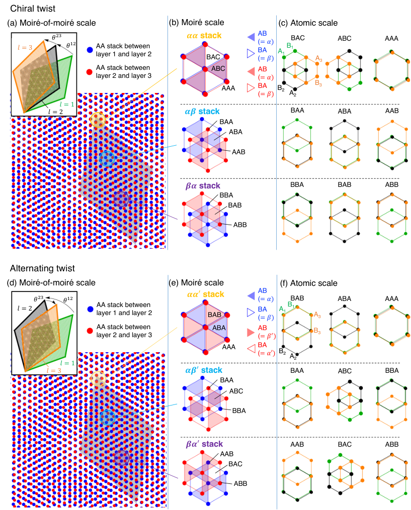
When absolute twist angles are close $(|\theta^{12}|\approx|\theta^{23}|)$, an interference between the two moiré patterns gives rise to a higher order structure called a moiré-of-moiré pattern as shown in Fig. 2. Here the upper and lower rows correspond to the chiral and alternating structures, respectively. For the chiral twist, the left panel [Fig. 2(a)] illustrates the overlapped moiré patterns where blue and red dots represent the AA spots of moiré 12 and 23, respectively. The local structure can be viewed as a pair of non-twisted moiré superlattices with a relative translation, as illustrated in Fig. 2(b). Here shaded and empty triangles represent AB, and BA stacking regions of individual moiré patterns, respectively. By defining AB and BA points (the centers of triangles) by $\alpha$ and $\beta$, respectively, the local stacking configuration of the two moiré patterns is labeled by $\alpha\alpha$, $\alpha\beta$ and $\beta\alpha$. Figure 2(c) depicts the local structure in the atomic scale. Here $A_{l}$ and $B_{l}$ represent the graphene’s sublattice in layer $l$. We define the sublattice $C_{l}$ as the center of the hexagon in the honeycomb lattice. For instance, BAC-stacking represents $B_{1}$, $A_{2}$ and $C_{3}$ are vertically aligned.

The lower panels [Figs. 2(d), (e) and (f)] are the corresponding figures for the alternate twist. The key difference from the chiral case lies in the 180^∘ rotation of the moiré 23 (red lattice) due to the opposing sign of $\theta^{23}$. This results in the flipping of the positions of AB and BA. Consequently, the local atomic structure (shown in the rightmost panels) differs between the chiral and alternating structures, even though the relative arrangement of AA spots is identical. We define AB and BA points in the inverted moiré 23 pattern by $\beta^{\prime}$ and $\alpha^{\prime}$, respectively, and label the local structure in the alternating TTG by $\alpha\alpha^{\prime}$, $\alpha\beta^{\prime}$ and $\beta\alpha^{\prime}$, as in Fig. 2(e).

Generally the two moiré patterns in a TTG are not commensurate, and the spatial period of moiré-of-moiré pattern is infinite. However, there are special angle sets $(\theta^{12},\theta^{23})$ where the two patterns happen to have a finite common period. In such a case, we can express the moiré-of-moiré primitive lattice vectors $\bm{L}_{1}$ and $\bm{L}_{2}$ in terms of integers $n,m,n^{\prime}$ and $m^{\prime}$ as

The moiré-of-moiré reciprocal lattice vectors are given by the condition $\bm{G}_{i}\cdot\bm{L}_{j}=2\pi\delta_{ij}$. The corresponding twist angles are obtained by solving Eqs. (1) and (II.2) for variables $\theta^{12}$ and $\theta^{23}$, as

where

The spatial period of the super-moiré pattern is given by $L=L^{12}\sqrt{n^{2}+m^{2}+nm}=L^{23}\sqrt{n^{\prime 2}+m^{\prime 2}+n^{\prime}m^{\prime}}$.

In alternating TTGs with $\theta^{12}\approx-\theta^{23}$, the relative angle between two moiré lattice vectors nearly vanishes, resulting in an extremely large commensurate moiré-of-moiré unit cell. To treat such cases, we neglect the tiny misorientation of the moiré lattice vectors $\bm{L}_{j}^{12}$ and $\bm{L}_{j}^{23}$, while retaining their norms. In this approximation, the moiré-of-moiré commensurate period is expressed as

instead of Eq.(II.2). Note that Eq. (3) does not apply to this approximate commensurate structure.

In this paper, we consider commensurate chiral TTGs, C1, C2 and C3, and commensurate alternating TTGs, A1, A2 and A3, defined in Table 1. We employ the exact commensurate formulas Eqs. (II.2) and (3) for C1, C2, C3, and A3, while we utilize the approximate formula, Eq. (5) for A1 and A2. Figure 3(a) maps $(\theta^{12},\theta^{23})$ of these systems in two-dimensional space, where the color code represents the ratio of the two moiré periods, $\min\left(L^{12}/L^{23},L^{23}/L^{12}\right)$. The moiré-of-moiré structures of these TTGs without lattice relaxation are illustrated in Fig. 3(b) and (c), respectively.

We show the schematics of Brillouin zone (BZ) of a chiral TTG in Fig. 4. Here green, black and orange hexagons represent the first BZ of layer 1, 2, and 3, respectively. Blue and red hexagons represent the BZ for the first moiré patterns given by $l=1,2$ and the second pattern given by $l=2,3$, respectively. Finally, the gray heaxagon is the BZ of the moiré-of-moiré pattern, where we label the corner points by $\kappa$ and $\kappa^{\prime}$, the midpoint of a side by $\mu$ and the center by $\gamma$.

We adopt a continuum approximation [72; 81; 82] to describe the lattice relaxation on TTG. Let $\bm{s}^{(l)}(\bm{R}_{X})$ be the displacement vector of sublattice $X=A$, or $B$ at a two-dimenisonal position $\bm{R}_{X}$ of layer $l=1,2,3$. Here we consider a long-rage lattice relaxation which has much longer scales than graphene’s lattice constant. The desplacement vectors can then be expressed by continuous functions in real space as $\bm{s}^{(l)}(\bm{R}_{A})=\bm{s}^{(l)}(\bm{R}_{B})=\bm{s}^{(l)}\left(\bm{r}\right)$. We ignore the out-of-plane component of the displacement vector in this model, as it does not much contribute to the commensurate domain formation. The optimized lattice structure can be obtained by minimizing the total energy $U=U_{E}+U_{B}^{12}+U_{B}^{23}$, where $U_{E}$ is the elastic energy and $U_{B}^{ll^{\prime}}$ is the interlayer binding energy between layers $l$ and $l^{\prime}$. We assume that $U_{B}^{12}$ and $U_{B}^{23}$ are given by the interlayer interaction energy of the twisted bilayer graphene [72], and neglect a remote interaction between layer 1 and 3. The $U_{E}$ and $U_{B}^{ll^{\prime}}$ can be expressed as funtionals of the displacement field $\bm{s}^{(l)}\left(\bm{r}\right)$. We solve the Euler-Lagrange equation to obtain the optimized $\bm{s}^{(l)}\left(\bm{r}\right)$ self-consistently.

The elastic energy of strained TTG is written in a standard form [83; 84] as

where $\lambda=3.25$ eV/$\AA^{2}$ and $\mu=9.57$ eV/$\AA^{2}$ are graphene’s Lamé factors[85; 70], and $s_{ij}^{(l)}=(\partial_{i}s_{j}^{(l)}+\partial_{j}s_{i}^{(l)})/2$ is the strain tensor. The interlayer binding energy of adjacent layers $(l,l^{\prime})=(1,2),(2,3)$ is given by [72]

where $\bm{b}_{3}=-\bm{b}_{1}-\bm{b}_{2}$, $\bm{G}_{3}^{ll^{\prime}}=-\bm{G}_{1}^{ll^{\prime}}-\bm{G}_{2}^{ll^{\prime}}$. We take $V_{0}=0.160$ eV/nm²[86; 87].

We introduce

and rewrite $U$ as a functional of $\bm{w},\bm{u}$ and $\bm{v}$. Here $\bm{w}$ represents an overall translation of three layers, while $\bm{u}$ and $\bm{v}$ are relative slidings which are mirror-even and odd, respectively, with respect to the middle layer. In the subsequent analysis, we fix $\bm{w}$ to zero and focus solely on $\bm{u}$ and $\bm{v}$, as $\bm{w}$ does not alter the interlayer registration and therefore does not impact the formation of moiré domains. The Euler-Lagrange equation is written as

where

We assume $\bm{s}^{(l)}$’s (so $\bm{u}$ and $\bm{v}$) are periodic in the original moiré-of-moiré period, and define the Fourier components as

where $\bm{G}=m_{1}\bm{G}_{1}+m_{2}\bm{G}_{2}$ are the moiré-of-moiré reciprocal lattice vectors. We also introduce $f_{\bm{G},j}^{ll^{\prime}}$ by

Eq. (II.3) is then written as

where

We obtain the optimized $\bm{u}_{\bm{G}}$ and $\bm{v}_{\bm{G}}$ by solving Eqs. (14) and (II.3) in an iterative manner. In the calculation, we only consider a finite number of the Fourier components in $|\bm{G}|<3\max\left(|n|,|m|,|n^{\prime}|,|m^{\prime}|\right)$, which are sufficient to describe the lattice relaxation in the systems considered. It should be noted that the components of $\bm{G}=0$ cannot be determined by this scheme, since $\hat{K}_{\bm{G}}$ becomes 0 in Eq. (II.3). Here we treat $\bm{s}^{(l)}_{\bm{G}=0}$ as parameters, and perform the above iteration for different parameter choices. We finally choose the solution having the lowest total energy. The dependence on $\bm{G}=0$ component arises because the moiré-of-moiré structure depends on a relative translation of the two moiré patterns, and hence it cannot be eliminated by a shift of the origin unlike twisted bilayer graphene. Practically, it is sufficient to consider only the lateral sliding of layer 3 with other two layers fixed.

We compute the band structure of the TTGs by using an electronic continuum model [88; 89; 90; 91; 92; 93] that incorporates lattice relaxation [77]. The effective Hamiltonian for valley $\xi$ is written as

The matrix works on a six-component wave function $(\psi_{A}^{(1)},\psi_{B}^{(1)},\psi_{A}^{(2)},\psi_{B}^{(2)},\psi_{A}^{(3)},\psi_{B}^{(3)})$, where $\psi_{X}^{(l)}$ represents the envelope function of sublattice $X(=A,B)$ on layer $l(=1,2,3)$. The $H_{l}(\bm{k})$ is the $2\times 2$ Hamiltonian of monolayer graphene and $U_{ll^{\prime}}$ is the interlayer coupling matrix, in the presence of the lattice distortion. The $H_{l}(\bm{k})$ is given by

where $v$ is the graphene’s band velocity, $\bm{\sigma}=\left(\xi\sigma_{x},\sigma_{y}\right)$ and $\sigma_{x}$, $\sigma_{y}$ are the Pauli matrices in the sublattice space $\left(A,B\right)$. We take $\hbar v/a=2.14$ eV [94]. The $\bm{A}^{(l)}$ is the strain-induced vector potential that is given by [83; 95; 96]

where $\gamma_{0}=2.7$ eV is the nearest neighbor transfer energy of intrinsic graphene and $\beta\approx 3.14$.

The interlayer coupling matrix $U_{21}$ and $U_{32}$ are given by

where we defined

and

The parameters $u=79.7$ meV and $u^{\prime}=95.7$ meV are interlayer coupling strength between AA/BB and AB/BA stack region, respectively[94; 97]. In the band calculation, we take Fourier components within the radius of $|\bm{G}|\leq 2\max\left(|n|,|m|,|n^{\prime}|,|m^{\prime}|\right)$ as the basis of Hamiltonian. We neglect remote interlayer hoppings between layer 1 and 3.

We study the lattice relaxation in the TTGs of C1$(1.79^{\circ},1.58^{\circ})$, C2$(2.64^{\circ},2.45^{\circ})$ and C3$(1.54^{\circ},0.64^{\circ})$ by using the method described in Sec. II.3. Figure 5 summarizes the optimized moiré structures for the three systems. In each row, the left panel shows the moiré pattern 12 (given by layer 1 and 2), and the middle panel shows moiré pattern 23 (by layer 2 and 3) after the relaxation. Here the color represents the local interlayer binding energy $U_{B}^{ll^{\prime}}$, where bright and dark regions correspond to the AA stack and AB/BA stack respectively. Tiny magenta dots indicate the original AA stack points without lattice relaxation for reference. In the right-most panel, we overlap the two moiré structures in a single diagram, where blue and red points represent the AA stack of the moiré 12 and 23 respectively. A rhombus in each panel represents the moiré-of-moiré unit cell, and all scale bars indicate 20 nm.

We first consider C1 and C2 which have relatively close twist angles $(\theta^{12},\theta^{23})$. In the rightmost panels of Fig. 5 (a) and (b), we see that locally-commensurate $\alpha\beta$ and $\beta\alpha$ domains (indicated by triangles) are formed. In these domains, the lattice relaxation equalizes the two moiré periods which were initially different, to achieve a commensurate structure. At the same time, we also have the lattice relaxation in a smaller scale as in twisted bilayer graphene, which shrinks AA regions and expands AB/BA regions in each of two moiré patterns. Therefore we have the relaxations in the moiré-of-moiré scale ($\alpha\beta$/$\beta\alpha$ domains) and in moiré scale (AB/BA domains) at the same time. The following questions naturally arise: (i) What distribution of displacement vectors leads to the multi-scale lattice relaxation? and (ii) Why does such a structure exhibit energetic preference? These questions can be answered by examining the obtained lattice displacement as follows.

Figure 6(a) shows the distribution of the displacement vector $\bm{s}^{(l)}(\bm{r})$ on layer 1, 2 and 3 for the case of C1. The middle row, Fig. 6(b), plots a coarse-grained component $\bar{\bm{s}}^{(l)}(\bm{r})$, which is calculated by averaging $\bm{s}^{(l)}(\bm{r})$ over a scale of moiré unit cell around the point $\bm{r}$. The bottom row [Fig.6(c)] displays magnified plots of $\bm{s}^{(l)}(\bm{r})-\bar{\bm{s}}^{(l)}(\bm{r})$ (i.e., the local component with the coarse-grained part subtracted) within the region enclosed by a dashed square in Fig.6(a).

In Fig. 6(b), we clearly see that $\bar{\bm{s}}^{(1)}$ and $\bar{\bm{s}}^{(3)}$ rotate counter-clockwise around the center of the $\alpha\beta$ and $\beta\alpha$ domains, while $\bar{\bm{s}}^{(2)}$ rotates in the clockwise direction. This behavior is closely linked to $\alpha\beta/\beta\alpha$ domain formation, and it can be comprehended by examining the problem in the $k$-space. Figure 7 depicts the relocation of BZ corners of layer 1, 2 and 3 in the C1 system under the lattice relaxation. The panel (a) is for the original non-distorted configuration. We define $\bm{q}_{1}^{12}=\bm{K}_{+}^{(2)}-\bm{K}_{+}^{(1)}$ and $\bm{q}_{1}^{23}=\bm{K}_{+}^{(3)}-\bm{K}_{+}^{(2)}$, where $\bm{K}_{+}^{(l)}$ is the BZ corner of layer $l$ near $\xi=+$ valley. The vectors $\bm{q}_{1}^{12}$ and $\bm{q}_{1}^{23}$ are associated with the periods of the moiré pattern 12 and that of 23, respectively. When these vectors are equal, two moiré periods completely match.

The lattice displacement in Fig. 6(b) works precisely to align the two vectors. In the case of C1, the angle between layer 1 and 2 is larger than the angle between layer 2 and 3 ($\theta^{12}>\theta^{23}$), so the layer 2 rotates clockwise, and the layer 1 and layer 3 rotate counter-clockwise to achieve $\theta^{12}=\theta^{23}$ [Fig. 7(b)]. There is still a tiny angle difference between $\bm{q}_{1}^{12}$ and $\bm{q}_{1}^{23}$. This can be eliminated by slightly expanding BZs layer 1 and 3, and shrinking BZ of layer 2, to finially obtain the perfect matching [Fig. 7(c)]. In the real space, this corresponds to a shrink of layer 1 and 3 and an expansion of layer 2. These changes are actually observed in Fig. 6(a), where the vector fields rotate around the center of the $\alpha\beta$/$\beta\alpha$ domain.

To understand the energetic stability of $\alpha\beta$/$\beta\alpha$ domains, we examine the local moiré-scale lattice relaxation. Let us first consider the twisted bilayer graphene, which has only a single moiré pattern. There the lattice relaxation takes place such that AB/BA stack region expands and AA stack region shrinks [72]. This is realized by a local interlayer rotation around AA and AB/BA stack points. Around AB/BA, specifically, the layer 1 and 2 oppositely rotate to reduce the local twist angle. The AB/BA region is then enlarged, because the length scale of the moiré pattern is enlarged in decreasing the twist angle. In AA spots, on the contrary, the layer 1 and 2 rotate to increase the local twist angle to shrink the AA region.

The same deformation occurs also in TTG, where all three layers undergo relaxation to expand AB/BA domain in each of the two moiré patterns. However, as the middle layer $l=2$ is shared by the two interference patterns, there can be a frustration such that, for instance, a local movement of the layer 2 leads to the expansion of the AB region in one moiré pattern while causing its contraction in the other. Therefore, the relative displacement of the two moiré superlattices should be determined in such a way that the middle-layer distortion can lower the total energies of the two moiré patterns at the same time.

Figure 8(a) is the schematic figure to illustrate the favorable local rotation of the middle layer, for the moiré 12 (between $l=1,2$) and moiré 23 (between $l=2,3$). The orange and green arc arrows correspond to clockwise and counterclockwise directions, respectively. Here we notice that the direction of rotation is opposite for moiré 12 and moiré 23, since layer 1 and layer 3 are originally twisted in opposite directions with respect to layer 2. When AA stack points of moiré 12 and moiré 23 are aligned ($\alpha\alpha$ stacking), the rotation direction of layer 2 is completely frustrated as shown in Fig. 8(b), and therefore $\alpha\alpha$ stacking is energetically unfavorable. The optimized structure is $\alpha\beta$ stacking [Fig. 8(c)], where the rotation angles coincide in two out of three regions.

When the two angles $\theta^{12}$ and $\theta^{23}$ are not close to each other, $\alpha\beta$/$\beta\alpha$ domains do not appear any more, but still a locally-commensurate moiré-of-moiré structure emerges. Figure 5(c) shows the relaxed structure for the C3 TTG. Since the unit areas of the two moiré patterns differ by nearly 3, we have commensurate domains where a single red triangle includes three blue triangles. We also see red AA points always come to the center of blue triangles. This can also be understood in terms of the alignment of the favorable rotation angles explained above.

Using the electronic continuum model introduced in Sec. II.4, we calculate the band structure of TTGs in the presence of the lattice relaxation. Figure 9(a) and (b) show the energy bands (near $K_{+}$ valley) and the corresponding density of states (DOS) calculated for the case C1 and C2, respectively. The labels $\kappa,\gamma,\mu,\kappa^{\prime}$ are symmetric points of the moiré-of-moiré BZ defined in Fig. 4.

We immediately notice that the spectrum exhibits distinct energy windows characterized by relatively low DOS, which span in the enegy range of 20 meV $<|E|<$ 90 meV for C1, and in 90 meV $<|E|<$ 180 meV for C2. The windows are sparsely filled with energy bands. Figure 9(c) shows the Fermi surface at $E_{F}=117$ meV in the C2, which is indicated by horizontal red line in Fig. 9(b). We see that the Fermi surface is composed of three intersecting lines arranged with a trigonal symmetry, indicating the dispersion is nearly one-dimensional. The band velocities of these one-dimensional bands (normal to the Fermi surface) are oriented to the moiré-of-moiré lattice vectors $\bm{L}_{1}$, $\bm{L}_{2}$ and $\bm{L}_{3}(=-\bm{L}_{1}+\bm{L}_{2})$. Figure 9(d) plots the distribution of the squared wave amplitudes of an eigenstate marked by a red point in Fig. 9(c). The wave function actually takes a highly one-dimensional form, and it is sharply localized within the domain walls dividing $\alpha\beta$ and $\beta\alpha$ regions. Each of the three Fermi surfaces corresponds to one-dimensional states running along the domain walls in the corresponding directions. The states with different directions are barely hybridized. We also have a low-DOS region near $E=0$ in the C2, while this is remnant of the graphene’s Dirac cone and the energy bands are not one-dimensional.

The existence of one-dimensional channels on the domain walls indicates that the $\alpha\beta$ and $\beta\alpha$ regions are locally gapped with different topological numbers, and associated topological boundary modes emerge between the domains, as shown in Fig. 1. To verify this, we calculate the bands structures and the Chern numbers of uniform TTG having $\alpha\beta/\beta\alpha$ stacking. The Hamiltonian of such a uniform system can be obtained by assuming the BZ-corner arrangement in Fig. 7(c), where $\bm{q}_{1}^{12}=\bm{q}_{1}^{23}\equiv\bm{q}$. This corresponds to a TTG where $\theta^{12}=\theta^{23}$ and the layer 2 is slightly expanded in relative to layer 1 and 3. The two moiré periods then become identical, and we have $\bm{G}_{j}^{12}=\bm{G}_{j}^{23}\equiv\bm{G}^{\rm M}_{j}$ and $\bm{q}=(2\bm{G}^{\rm M}_{1}+\bm{G}^{\rm M}_{2})/3$. The Hamiltonian for this system is obtained from Eq. (II.4) as

where

and we neglect the strain-induced vector potentials which does not affect the topological nature argued here. Here $U_{21}$ and $U_{32}$ differ by the parameter $\bm{r}_{0}$, which specifies the relative displacement between the two moiré patterns. The $\alpha\beta$ and $\beta\alpha$ stackings correspond to $\bm{r}_{0}=\left(\bm{L}_{1}^{M}+\bm{L}_{2}^{M}\right)/3$ and $2\left(\bm{L}_{1}^{M}+\bm{L}_{2}^{M}\right)/3$ respectively, where $\bm{L}_{j}^{M}$ is the common moiré lattice vector given by $\bm{G}_{i}^{M}\cdot\bm{L}_{j}^{M}=2\pi\delta_{ij}$.

Here we consider uniform $\alpha\beta$ and $\beta\alpha$ TTGs with $\theta^{12}=\theta^{23}=2.54^{\circ}$, which approximate the local structures of $\alpha\beta$ and $\beta\alpha$ domains in the C2. Figure 10 plots the energy bands in $\xi=+$ valley calculated by Eq. (III.2). We observe energy gaps in the electron and hole sides in the region $50\,{\rm meV}<|E|<180\,{\rm meV}$, which approximately coincides with the energy window of the C2 [Fig. 9(b)]. Between the gaps in the electron and hole sides, we have two bands touching at the charge neutrality point. The total Chern number for the two-band cluster is found to be $\mp 1$ for $\alpha\beta$ and $\beta\alpha$, respectively. The absolute Chern number in the upper gap can also be calculated, and it turns out to be $\mp 1/2$ for $\alpha\beta$ and $\beta\alpha$, respectively. This is obtained by opening mass gap (adding asymmetric energies to A and B sublattices in all the graphene layers) to lift the band touching at the Dirac point. Since the difference of the Chern number of the upper gap between the $\alpha\beta$ and $\beta\alpha$ regions is 1, we have a single edge mode (per a single valley) at the domain boundary. This coincides with the number of the one-dimenisonal modes per a single direction in the moiré-of-moiré superlattice band Fig. 9. The Chern number of the valley $\xi=-1$ is negative of $\xi=+1$ valley due to the time reversal symmetry. Therefore the TTG is a quantized valley Hall insulator when the Fermi energy is in the energy window.

The energy windows and one-dimensional domain-wall states also appear in the C1 case [Fig. 9(a)], which has a smaller moiré-of-moiré period. The degree of one-dimensionality is not as pronounced as in the C2 configuration, as evidenced by the appearance of small gaps at the intersections of bands. The hybridization tends to be greater when the moiré-of-moiré period is smaller.

Finally, the band structure in Fig. 9 closely resembles the marginally-stacked twisted bilayer graphene in a strong perpendicular electric field [98; 99; 100; 101; 102; 103; 104]. There the topological one dimensional edge states arise since the AB and BA regions in the moiré pattern have opposite valley Chern numbers in the electric field. The chiral TTG realizes a similar situation in the moiré-of-moiré scale, without the need for an applied electric field. This can be achieved in any chiral TTGs where $\theta^{12}$ and $\theta^{23}$ are close to each other, such that the two moiré periods are comparable.

Alternating TTGs display distinct relaxed structures that differ entirely from the chiral cases. Figure 11 shows optimized moiré structures calculated for alternating TTGs (a) A1 $(\theta^{12},\theta^{23})=(1.48^{\circ},-1.18^{\circ})$, (b) A2 $(1.42^{\circ},-1.22^{\circ})$ and (c) A3 $(1.47^{\circ},-0.62^{\circ})$, corresponding to Fig. 5 for chiral TTGs. In the A1 and A2, we observe a formation of commensurate $\alpha\alpha^{\prime}$ domains, where AA spots of the two moiré patterns completely overlaps [See Fig. 2(e)]. This is in a sharp contrast to the chiral TTGs, where AA spots are repelled to each other, giving rise to $\alpha\beta/\beta\alpha$ domains. The atomic structure of $\alpha\alpha^{\prime}$ domain corresponds precisely to the mirror-symmetric TTG with $\theta^{12}=-\theta^{23}$. In A3 case [Fig. 11(c)], where the two moiré periods are not comparable, we observe a different type of commensurate domain with the ratio of the lattice periods fixed at 2, reflecting the original moiré-period ratio $L^{23}/L^{12}\simeq 2.3$. Here the AA stacking points of the red and blue moiré lattices are vertically aligned as in $\alpha\alpha^{\prime}$ domains observed in A1 and A2.

The formation of the commensurate domains can be attributed to a specific type of lattice distortion that differs from the chiral case. Figure 12 shows the distribution of the coarse-grained displacement vector $\bar{\bm{s}}^{(l)}(\bm{r})$ in the A1 case (corresponding to Fig. 6(b) for the chiral case). We observe that the layer 1 and layer 3 rotate anti-clockwise and clock-wise directions, respectively, around $\alpha\alpha^{\prime}$ domain center. In $k$-space, accordingly, the Brillouin zone corners of layer 1 and 3 move to overlap as shown in Fig. 13. This corresponds to the symmetric TTG $(\theta^{12}=-\theta^{23})$ where the layer 1 and layer 3 are perfectly aligned.

The stability of $\alpha\alpha^{\prime}$-domain is also explained by considering moiré-scale lattice relaxation. As discussed in Sec. III.1, the graphene layers in TTG undergo spontaneous distortion to expand the AB/BA regions for the moiré patterns 12 and 23, giving a competitive environment for the shared layer 2. Figure 14(a) depicts the preferred orientation of layer 2 for the two moiré patterns in alternating TTG. In contrast to the chiral stack [Fig. 8], the rotation direction is identical for both moiré patterns, since layer 1 and layer 3 are rotated in the same direction relative to the layer 2. Consequently, there is no frustration when the moiré lattices are arranged in an $\alpha\alpha^{\prime}$ stack as shown in Fig. 14(b). In this structure, the motion of the shared layer 2 allows for the simultaneous relaxation of the moiré patterns 12 and 23, resulting in an energy advantage compared to partially frustrated configurations like the $\alpha\beta^{\prime}$ stack [Fig. 14(c)]. The stability of $\alpha\alpha^{\prime}$ stack in nearly-symmetric TTGs was pointed out in the previous theoretical works [22; 26; 47; 48], and it was observed in recent experiments [78; 80].

We calculate the band structure for alternating TTGs of A1$(1.48^{\circ},-1.18^{\circ})$, (b)A2$(1.42^{\circ},-1.22^{\circ})$ using the method described in Sec. II. The energy band and DOS for A1 and A2 are displayed in Figs. 15(a) and (b), respectively. In each figure, the right and left panels correspond to the TTGs with and without the lattice relaxation, respectively. Black curves represent the energy bands, and blue straight lines indicate the intrinsic Dirac bands of layer 1 and layer 3 without the interlayer coupling. Red dots indicate the amplitude projected onto the mirror-odd plane wave states, as defined by

where $\psi_{n\bm{k}}$ is the eigenstates, and $|\bm{k},X,l\rangle$ is the plane wave at sublattice $X(=A,B)$ on layer $l$. We take the path $\bm{K}_{+}^{(1)}\to\bm{K}_{+}^{(3)}\to\bm{K}_{+}^{(2)}$ on a straight line in the extended $k$-space, as shown in insets of Fig. 15.

In the band structures with the lattice relaxation, we observe numerous flat bands concentrated around zero energy, and these bands are surrounded by a region where dispersive energy bands are sparsely distributed. These features coincide with the mirror-symmetric TTG $(\theta^{12}=-\theta^{23})$, where the low-energy spectrum is composed of a flat band with even parity, and a Dirac cone with odd parity against the mirror inversion [21; 22]. We see that the red dots roughly form a conical dispersion, and it is regarded as a remnant of the symmetric TTG’s Dirac cone having odd parity. In the non-relaxed calculations, we notice that the flat bands and Dirac cones are strongly hybridized, and the conical dispersion of the red dots is not clearly resolved. These results suggest that the formation of $\alpha\alpha^{\prime}$ domains (equivalent to the mirror-symmetric TTG) supports the spectral separation of the flat bands and the Dirac-cone like bands. Therefore, we expect that asymmetric TTGs slightly away from the symmetric condition $\theta^{12}=-\theta^{23}$ acquire similar electronic properties to the symmetric TTG, through the moiré-of-moiré lattice relaxation.

The electronic properties of TTG can be tuned by applying a perpendicular electric field. We can introduce the field effect to our model as $H+V$, where $H$ is the original Hamiltonian of Eq. (II.4), and $V$ is the on-site potential term by perpendicular electronic field,

Here $\Delta$ is the difference of the on-site energy and $\hat{I}_{2}$ is a $2\times 2$ unit matrix, and we simply assumed the perpendicular electric field is constant between top layer and bottom layer. Figure 16 shows the energy band of the A2 with lattice relaxation, under the perpendicular electric field $\Delta=50$ meV and $100$ meV. When the electric field is applied, we observe the Dirac band moves along the energy axes, and eventually the Dirac point emerges out of the flat-band cluster. We also see that the electric fields broadens the energy width of the flat band region, and enhances a hybridization between the flat bands and the dispersive bands.

References

- Cao et al. [2018a] Y. Cao, V. Fatemi, A. Demir, S. Fang, S. L. Tomarken, J. Y. Luo, J. D. Sanchez-Yamagishi, K. Watanabe, T. Taniguchi, E. Kaxiras, R. C. Ashoori, and P. Jarillo-Herrero, Nature 556, 80 (2018a).
- Cao et al. [2018b] Y. Cao, V. Fatemi, S. Fang, K. Watanabe, T. Taniguchi, E. Kaxiras, and P. Jarillo-Herrero, Nature 556, 43 (2018b).
- Yankowitz et al. [2019] M. Yankowitz, S. Chen, H. Polshyn, Y. Zhang, K. Watanabe, T. Taniguchi, D. Graf, A. F. Young, and C. R. Dean, Science 363, 1059 (2019), https://www.science.org/doi/pdf/10.1126/science.aav1910 .
- Kerelsky et al. [2019] A. Kerelsky, L. J. McGilly, D. M. Kennes, L. Xian, M. Yankowitz, S. Chen, K. Watanabe, T. Taniguchi, J. Hone, C. Dean, A. Rubio, and A. N. Pasupathy, Nature 572, 95 (2019).
- Xie et al. [2019] Y. Xie, B. Lian, B. Jäck, X. Liu, C.-L. Chiu, K. Watanabe, T. Taniguchi, B. A. Bernevig, and A. Yazdani, Nature 572, 101 (2019).
- Jiang et al. [2019] Y. Jiang, X. Lai, K. Watanabe, T. Taniguchi, K. Haule, J. Mao, and E. Y. Andrei, Nature 573, 91 (2019).
- Polshyn et al. [2019] H. Polshyn, M. Yankowitz, S. Chen, Y. Zhang, K. Watanabe, T. Taniguchi, C. R. Dean, and A. F. Young, Nature Physics 15, 1011 (2019).
- Choi et al. [2019] Y. Choi, J. Kemmer, Y. Peng, A. Thomson, H. Arora, R. Polski, Y. Zhang, H. Ren, J. Alicea, G. Refael, F. von Oppen, K. Watanabe, T. Taniguchi, and S. Nadj-Perge, Nature Physics 15, 1174 (2019).
- Sharpe et al. [2019] A. L. Sharpe, E. J. Fox, A. W. Barnard, J. Finney, K. Watanabe, T. Taniguchi, M. A. Kastner, and D. Goldhaber-Gordon, Science 365, 605 (2019), https://www.science.org/doi/pdf/10.1126/science.aaw3780 .
- Lu et al. [2019] X. Lu, P. Stepanov, W. Yang, M. Xie, M. A. Aamir, I. Das, C. Urgell, K. Watanabe, T. Taniguchi, G. Zhang, A. Bachtold, A. H. MacDonald, and D. K. Efetov, Nature 574, 653 (2019).
- Cao et al. [2020] Y. Cao, D. Chowdhury, D. Rodan-Legrain, O. Rubies-Bigorda, K. Watanabe, T. Taniguchi, T. Senthil, and P. Jarillo-Herrero, Phys. Rev. Lett. 124, 076801 (2020).
- Serlin et al. [2020] M. Serlin, C. L. Tschirhart, H. Polshyn, Y. Zhang, J. Zhu, K. Watanabe, T. Taniguchi, L. Balents, and A. F. Young, Science 367, 900 (2020), https://www.science.org/doi/pdf/10.1126/science.aay5533 .
- Chen et al. [2020] G. Chen, A. L. Sharpe, E. J. Fox, Y.-H. Zhang, S. Wang, L. Jiang, B. Lyu, H. Li, K. Watanabe, T. Taniguchi, et al., Nature 579, 56 (2020).
- Saito et al. [2020] Y. Saito, J. Ge, K. Watanabe, T. Taniguchi, and A. F. Young, Nature Physics 16, 926 (2020).
- Zondiner et al. [2020] U. Zondiner, A. Rozen, D. Rodan-Legrain, Y. Cao, R. Queiroz, T. Taniguchi, K. Watanabe, Y. Oreg, F. von Oppen, A. Stern, et al., Nature 582, 203 (2020).
- Wong et al. [2020] D. Wong, K. P. Nuckolls, M. Oh, B. Lian, Y. Xie, S. Jeon, K. Watanabe, T. Taniguchi, B. A. Bernevig, and A. Yazdani, Nature 582, 198 (2020).
- Stepanov et al. [2020] P. Stepanov, I. Das, X. Lu, A. Fahimniya, K. Watanabe, T. Taniguchi, F. H. Koppens, J. Lischner, L. Levitov, and D. K. Efetov, Nature 583, 375 (2020).
- Arora et al. [2020] H. S. Arora, R. Polski, Y. Zhang, A. Thomson, Y. Choi, H. Kim, Z. Lin, I. Z. Wilson, X. Xu, J.-H. Chu, et al., Nature 583, 379 (2020).
- Stepanov et al. [2021] P. Stepanov, M. Xie, T. Taniguchi, K. Watanabe, X. Lu, A. H. MacDonald, B. A. Bernevig, and D. K. Efetov, Phys. Rev. Lett. 127, 197701 (2021).
- Mora et al. [2019] C. Mora, N. Regnault, and B. A. Bernevig, Phys. Rev. Lett. 123, 026402 (2019).
- Li et al. [2019] X. Li, F. Wu, and A. H. MacDonald, “Electronic structure of single-twist trilayer graphene,” (2019), arXiv:1907.12338 [cond-mat.mtrl-sci] .
- Carr et al. [2020] S. Carr, C. Li, Z. Zhu, E. Kaxiras, S. Sachdev, and A. Kruchkov, Nano Letters 20, 3030 (2020), pMID: 32208724, https://doi.org/10.1021/acs.nanolett.9b04979 .
- Tritsaris et al. [2020] G. A. Tritsaris, S. Carr, Z. Zhu, Y. Xie, S. B. Torrisi, J. Tang, M. Mattheakis, D. T. Larson, and E. Kaxiras, 2D Materials 7, 035028 (2020).
- Lopez-Bezanilla and Lado [2020] A. Lopez-Bezanilla and J. L. Lado, Phys. Rev. Res. 2, 033357 (2020).
- Ramires and Lado [2021] A. Ramires and J. L. Lado, Phys. Rev. Lett. 127, 026401 (2021).
- Lei et al. [2021] C. Lei, L. Linhart, W. Qin, F. Libisch, and A. H. MacDonald, Phys. Rev. B 104, 035139 (2021).
- Phong et al. [2021] V. o. T. Phong, P. A. Pantaleón, T. Cea, and F. Guinea, Phys. Rev. B 104, L121116 (2021).
- Călugăru et al. [2021] D. Călugăru, F. Xie, Z.-D. Song, B. Lian, N. Regnault, and B. A. Bernevig, Phys. Rev. B 103, 195411 (2021).
- Xie et al. [2021] F. Xie, N. Regnault, D. Călugăru, B. A. Bernevig, and B. Lian, Phys. Rev. B 104, 115167 (2021).
- Guerci et al. [2022] D. Guerci, P. Simon, and C. Mora, Phys. Rev. Res. 4, L012013 (2022).
- Christos et al. [2022] M. Christos, S. Sachdev, and M. S. Scheurer, Phys. Rev. X 12, 021018 (2022).
- Zhang et al. [2022] Y. Zhang, R. Polski, C. Lewandowski, A. Thomson, Y. Peng, Y. Choi, H. Kim, K. Watanabe, T. Taniguchi, J. Alicea, F. von Oppen, G. Refael, and S. Nadj-Perge, Science 377, 1538 (2022), https://www.science.org/doi/pdf/10.1126/science.abn8585 .
- Hao et al. [2021] Z. Hao, A. M. Zimmerman, P. Ledwith, E. Khalaf, D. H. Najafabadi, K. Watanabe, T. Taniguchi, A. Vishwanath, and P. Kim, Science 371, 1133 (2021), https://www.science.org/doi/pdf/10.1126/science.abg0399 .
- Park et al. [2021] J. M. Park, Y. Cao, K. Watanabe, T. Taniguchi, and P. Jarillo-Herrero, Nature 590, 249 (2021).
- Cao et al. [2021] Y. Cao, J. M. Park, K. Watanabe, T. Taniguchi, and P. Jarillo-Herrero, Nature 595, 526 (2021).
- Kim et al. [2022] H. Kim, Y. Choi, C. Lewandowski, A. Thomson, Y. Zhang, R. Polski, K. Watanabe, T. Taniguchi, J. Alicea, and S. Nadj-Perge, Nature 606, 494 (2022).
- Zhu et al. [2020a] Z. Zhu, P. Cazeaux, M. Luskin, and E. Kaxiras, Phys. Rev. B 101, 224107 (2020a).
- Zhu et al. [2020b] Z. Zhu, S. Carr, D. Massatt, M. Luskin, and E. Kaxiras, Phys. Rev. Lett. 125, 116404 (2020b).
- Lin et al. [2020] F. Lin, J. Qiao, J. Huang, J. Liu, D. Fu, A. S. Mayorov, H. Chen, P. Mukherjee, T. Qu, C.-H. Sow, et al., Nano Letters 20, 7572 (2020).
- Zhang et al. [2021] X. Zhang, K.-T. Tsai, Z. Zhu, W. Ren, Y. Luo, S. Carr, M. Luskin, E. Kaxiras, and K. Wang, Phys. Rev. Lett. 127, 166802 (2021).
- Gao and Khalaf [2022] Q. Gao and E. Khalaf, Physical Review B 106, 075420 (2022).
- Ma et al. [2022] Z. Ma, S. Li, M. Lu, D.-H. Xu, J.-H. Gao, and X. Xie, Science China Physics, Mechanics & Astronomy 66, 227211 (2022).
- Liang et al. [2022] M. Liang, M.-M. Xiao, Z. Ma, and J.-H. Gao, Phys. Rev. B 105, 195422 (2022).
- Uri et al. [2023] A. Uri, S. C. de la Barrera, M. T. Randeria, D. Rodan-Legrain, T. Devakul, P. J. D. Crowley, N. Paul, K. Watanabe, T. Taniguchi, R. Lifshitz, L. Fu, R. C. Ashoori, and P. Jarillo-Herrero, “Superconductivity and strong interactions in a tunable moiré quasiperiodic crystal,” (2023), arXiv:2302.00686 [cond-mat.mes-hall] .
- Mao et al. [2023] Y. Mao, D. Guerci, and C. Mora, Phys. Rev. B 107, 125423 (2023).
- Popov and Tarnopolsky [2023] F. K. Popov and G. Tarnopolsky, “Magic angles in equal-twist trilayer graphene,” (2023), arXiv:2303.15505 [cond-mat.str-el] .
- Lin et al. [2022] X. Lin, C. Li, K. Su, and J. Ni, Phys. Rev. B 106, 075423 (2022).
- Meng et al. [2023] H. Meng, Z. Zhan, and S. Yuan, Phys. Rev. B 107, 035109 (2023).
- Oka and Koshino [2021] H. Oka and M. Koshino, Physical Review B 104, 035306 (2021).
- Koshino and Oka [2022] M. Koshino and H. Oka, Physical Review Research 4, 013028 (2022).
- Finney et al. [2019] N. R. Finney, M. Yankowitz, L. Muraleetharan, K. Watanabe, T. Taniguchi, C. R. Dean, and J. Hone, Nature nanotechnology 14, 1029 (2019).
- Wang et al. [2019a] L. Wang, S. Zihlmann, M.-H. Liu, P. Makk, K. Watanabe, T. Taniguchi, A. Baumgartner, and C. Schönenberger, Nano letters 19, 2371 (2019a).
- Wang et al. [2019b] Z. Wang, Y. B. Wang, J. Yin, E. Tóvári, Y. Yang, L. Lin, M. Holwill, J. Birkbeck, D. Perello, S. Xu, et al., Science advances 5, eaay8897 (2019b).
- Yang et al. [2020] Y. Yang, J. Li, J. Yin, S. Xu, C. Mullan, T. Taniguchi, K. Watanabe, A. K. Geim, K. S. Novoselov, and A. Mishchenko, arXiv preprint arXiv:2010.03798 (2020).
- Andelkovic et al. [2020] M. Andelkovic, S. P. Milovanovic, L. Covaci, and F. M. Peeters, Nano letters 20, 979 (2020).
- Leconte and Jung [2020] N. Leconte and J. Jung, 2D Materials 7, 031005 (2020).
- Onodera et al. [2020] M. Onodera, K. Kinoshita, R. Moriya, S. Masubuchi, K. Watanabe, T. Taniguchi, and T. Machida, Nano letters 20, 4566 (2020).
- Kuiri et al. [2021] M. Kuiri, S. K. Srivastav, S. Ray, K. Watanabe, T. Taniguchi, T. Das, and A. Das, Physical Review B 103, 115419 (2021).
- Shi et al. [2021] J. Shi, J. Zhu, and A. MacDonald, Physical Review B 103, 075122 (2021).
- Shin et al. [2021a] J. Shin, Y. Park, B. L. Chittari, J.-H. Sun, and J. Jung, Physical Review B 103, 075423 (2021a).
- Shin et al. [2021b] J. Shin, B. L. Chittari, and J. Jung, Physical Review B 104, 045413 (2021b).
- Huang et al. [2021] X. Huang, L. Chen, S. Tang, C. Jiang, C. Chen, H. Wang, Z.-X. Shen, H. Wang, and Y.-T. Cui, arXiv preprint arXiv:2102.08594 (2021).
- Popov et al. [2011a] A. M. Popov, I. V. Lebedeva, A. A. Knizhnik, Y. E. Lozovik, and B. V. Potapkin, Phys. Rev. B 84, 045404 (2011a).
- Brown et al. [2012] L. Brown, R. Hovden, P. Huang, M. Wojcik, D. A. Muller, and J. Park, Nano Lett. 12, 1609 (2012).
- Lin et al. [2013] J. Lin, W. Fang, W. Zhou, A. R. Lupini, J. C. Idrobo, J. Kong, S. J. Pennycook, and S. T. Pantelides, Nano Lett. 13, 3262 (2013).
- Alden et al. [2013] J. S. Alden, A. W. Tsen, P. Y. Huang, R. Hovden, L. Brown, J. Park, D. A. Muller, and P. L. McEuen, Proc. Natl. Acad. Sci. USA 110, 11256 (2013).
- Uchida et al. [2014] K. Uchida, S. Furuya, J.-I. Iwata, and A. Oshiyama, Phys. Rev. B 90, 155451 (2014).
- van Wijk et al. [2015] M. van Wijk, A. Schuring, M. Katsnelson, and A. Fasolino, 2D Mater. 2, 034010 (2015).
- Dai et al. [2016] S. Dai, Y. Xiang, and D. J. Srolovitz, Nano Lett. 16, 5923 (2016).
- Jung et al. [2015] J. Jung, A. M. DaSilva, A. H. MacDonald, and S. Adam, Nat. Commun. 6, 6308 (2015).
- Jain et al. [2016] S. K. Jain, V. Juričić, and G. T. Barkema, 2D Mater. 4, 015018 (2016).
- Nam and Koshino [2017] N. N. T. Nam and M. Koshino, Phys. Rev. B 96, 075311 (2017), errata ibid 101, 099901 (2020).
- Carr et al. [2018] S. Carr, D. Massatt, S. B. Torrisi, P. Cazeaux, M. Luskin, and E. Kaxiras, Phys. Rev. B 98, 224102 (2018).
- Lin et al. [2018] X. Lin, D. Liu, and D. Tománek, Phys. Rev. B 98, 195432 (2018).
- Yoo et al. [2019] H. Yoo, R. Engelke, S. Carr, S. Fang, K. Zhang, P. Cazeaux, S. H. Sung, R. Hovden, A. W. Tsen, T. Taniguchi, G.-C. Watanabe, Kenji Yi, M. Kim, L. Mitchell, E. B. Tadmor, E. Kaxiras, and P. Kim, Nat. Mater. 18, 448 (2019).
- Guinea and Walet [2019] F. Guinea and N. R. Walet, Phys. Rev. B 99, 205134 (2019).
- Koshino and Nam [2020a] M. Koshino and N. N. Nam, Phys. Rev. B 101, 195425 (2020a).
- Turkel et al. [2022] S. Turkel, J. Swann, Z. Zhu, M. Christos, K. Watanabe, T. Taniguchi, S. Sachdev, M. S. Scheurer, E. Kaxiras, C. R. Dean, and A. N. Pasupathy, Science 376, 193 (2022), https://www.science.org/doi/pdf/10.1126/science.abk1895 .
- Li et al. [2022] Y. Li, M. Xue, H. Fan, C.-F. Gao, Y. Shi, Y. Liu, K. Watanabe, T. Tanguchi, Y. Zhao, F. Wu, et al., Nano Letters 22, 6215 (2022).
- Craig et al. [2023] I. M. Craig, M. V. Winkle, C. Groschner, K. Zhang, N. Dowlatshahi, Z. Zhu, T. Taniguchi, K. Watanabe, S. M. Griffin, and D. K. Bediako, “Local atomic stacking and symmetry in twisted graphene trilayers,” (2023), arXiv:2303.09662 [cond-mat.mes-hall] .
- Koshino and Son [2019] M. Koshino and Y.-W. Son, Phys. Rev. B 100, 075416 (2019).
- Krisna and Koshino [2023] L. P. A. Krisna and M. Koshino, Phys. Rev. B 107, 115301 (2023).
- Suzuura and Ando [2002] H. Suzuura and T. Ando, Phys. Rev. B 65, 235412 (2002).
- San-Jose et al. [2014] P. San-Jose, A. Gutiérrez-Rubio, M. Sturla, and F. Guinea, Phys. Rev. B 90, 115152 (2014).
- Zakharchenko et al. [2009] K. V. Zakharchenko, M. I. Katsnelson, and A. Fasolino, Phys. Rev. Lett. 102, 046808 (2009).
- Popov et al. [2011b] A. M. Popov, I. V. Lebedeva, A. A. Knizhnik, Y. E. Lozovik, and B. V. Potapkin, Phys. Rev. B 84, 045404 (2011b).
- Lebedeva et al. [2011] I. V. Lebedeva, A. A. Knizhnik, A. M. Popov, Y. E. Lozovik, and B. V. Potapkin, Physical Chemistry Chemical Physics 13, 5687 (2011).
- Lopes dos Santos et al. [2007] J. Lopes dos Santos, N. Peres, and A. Castro Neto, Phys. Rev. Lett. 99, 256802 (2007).
- Bistritzer and MacDonald [2011] R. Bistritzer and A. MacDonald, Proc. Natl. Acad. Sci. 108, 12233 (2011).
- Kindermann and First [2011] M. Kindermann and P. First, Phys. Rev. B 83, 045425 (2011).
- Lopes dos Santos et al. [2012] J. M. B. Lopes dos Santos, N. M. R. Peres, and A. H. Castro Neto, Phys. Rev. B 86, 155449 (2012).
- Moon and Koshino [2013] P. Moon and M. Koshino, Phys. Rev. B 87, 205404 (2013).
- Koshino [2015] M. Koshino, New J. Phys. 17, 015014 (2015).
- Koshino et al. [2018] M. Koshino, N. F. Q. Yuan, T. Koretsune, M. Ochi, K. Kuroki, and L. Fu, Phys. Rev. X 8, 031087 (2018).
- Pereira and Castro Neto [2009] V. M. Pereira and A. H. Castro Neto, Phys. Rev. Lett. 103, 046801 (2009).
- Guinea et al. [2010] F. Guinea, M. I. Katsnelson, and A. K. Geim, Nature Physics 6, 30 (2010).
- Koshino and Nam [2020b] M. Koshino and N. N. T. Nam, Phys. Rev. B 101, 195425 (2020b).
- San-Jose and Prada [2013] P. San-Jose and E. Prada, Phys. Rev. B 88, 121408 (2013).
- Ramires and Lado [2018] A. Ramires and J. L. Lado, Phys. Rev. Lett. 121, 146801 (2018).
- Efimkin and MacDonald [2018] D. K. Efimkin and A. H. MacDonald, Phys. Rev. B 98, 035404 (2018).
- Fleischmann et al. [2020] M. Fleischmann, R. Gupta, F. Wullschlägger, S. Theil, D. Weckbecker, V. Meded, S. Sharma, B. Meyer, and S. Shallcross, Nano Lett. 20, 971 (2020).
- Walet and Guinea [2019] N. R. Walet and F. Guinea, 2D Materials 7, 015023 (2019).
- Tsim et al. [2020] B. Tsim, N. N. T. Nam, and M. Koshino, Phys. Rev. B 101, 125409 (2020).
- Hou et al. [2020] T. Hou, Y. Ren, Y. Quan, J. Jung, W. Ren, and Z. Qiao, Phys. Rev. B 101, 201403 (2020).
- Devakul et al. [2023] T. Devakul, P. J. Ledwith, L.-Q. Xia, A. Uri, S. de la Barrera, P. Jarillo-Herrero, and L. Fu, arXiv preprint arXiv:2305.03031 (2023).
- Guerci et al. [2023] D. Guerci, Y. Mao, and C. Mora, arXiv preprint arXiv:2305.03702 (2023).