DEGREE: Decomposition Based Explanation for Graph Neural Networks

We first introduce the notations used in this work. Given a graph $\mathcal{G}=(\mathcal{V},\mathcal{E})$, where $\mathcal{V}$ is the set of nodes and $\mathcal{E}$ is the set of edges between nodes. The adjacency matrix of $\mathcal{G}$ is denoted as $\mathbf{A}\in\mathbb{R}^{N\times N}$, where $N=|\mathcal{V}|$ is the number of nodes, so $\mathcal{V}=\{v_{1},v_{2},...,v_{N}\}$. The nodes are associated with features, and the feature matrix is denoted as $\mathbf{X}\in\mathbb{R}^{N\times F}$, where $F$ is the feature dimension.

In this work, we focus on explaining GNN-based classification models. Let $f$ denote the target GNN model. $f$ computes the likelihood of a node or graph belonging to the target class, where $f\mathrel{\mathop{\mathchar 58\relax}}\mathcal{G}\mapsto\mathbb{R}^{\left|\mathcal{V}\right|}$ or $f\mathrel{\mathop{\mathchar 58\relax}}\mathcal{G}\mapsto\mathbb{R}$, for node or graph classification respectively.

The goal of explanation is to find the most important subgraph in $\mathcal{G}$ given $f(\mathcal{G})$, which requires measuring the contribution of all possible subgraphs and find the ones with high contribution scores. However, there are two challenges to be addressed. (1) Given any subgraph of interest, how to estimate its contribution without breaking up the input graph? (2) The number of all subgraphs in $\mathcal{G}$ is usually very large, so how to choose candidate subgraphs for improving explanation efficiency? We tackle the first challenge in the following part of Sec 3 and solve the second one in Sec 4.

In general, a prediction model $f$ contains multiple layers $L_{t},t\in\{1,\ldots,T\}$:

Let $\mathbf{X}[t]$ denotes the input to $L_{t}$, so $\mathbf{X}[t+1]=L_{t}(\mathbf{X}[t])$ and $\mathbf{X}[1]=\mathbf{X}$. The symbol $\circ$ denotes function composition. Here $\mathbf{X}[t]\in\mathbb{R}^{N\times F_{t}}$ is the embedding matrix at $t$-th layer, where $F_{t}$ is the latent dimension. The embedding vector of the $i$-th node at $t$-th layer is denoted as $\mathbf{X}_{i}[t]$.

The core idea of decomposition based explanation is that, given a target node group (or subgraph) of interest, we estimate its contribution score to model prediction merely through feed-forward propagation. We call the information propagated from the target group as target portion, and the rest of information is called background portion. It is worth noting that, a node is in the target group does not necessarily mean it is important, while it only means we are interested in its importance score. In the following, we use $\gamma$ and $\beta$ to denote the target and background portion, respectively. Let $\mathbf{m}\in\{0,1\}^{N}$, where $\mathbf{m}_{i}=1$ means $v_{i}$ belongs to the target group and otherwise $\mathbf{m}_{i}=0$. Then, the decomposition is initialized from the layer of node features, where the target portion and background portion of the input feature matrix are: $\mathbf{X}^{\gamma}=diag(\mathbf{m})\mathbf{X}$ and $\mathbf{X}^{\beta}=(\mathbf{I}-diag(\mathbf{m}))\mathbf{X}$, respectively. In a neural network, information from different parts of input are merged in the feedforward process into latent representations, which poses challenges for explanation. Suppose the target and background portion in $\mathbf{X}[t]$ are known from prior layer, we could explain the model if we can still distinguish the information flows of the two portions inside $L_{t}$. That is, at layer $L_{t}$, suppose its input can be decomposed as $\mathbf{X}[t]=\mathbf{X}^{\gamma}[t]+\mathbf{X}^{\beta}[t]$, the following relations need to hold for explanation:

where $L_{t}^{D}(\cdot,\cdot)$ denotes the decomposed version of layer $L_{t}$. $\Gamma(\cdot,\cdot)$ and $B(\cdot,\cdot)$ corresponds to the contribution of the target and the background portion to layer $L_{t}$. $\mathbf{X}^{\gamma}[t+1]$ and $\mathbf{X}^{\beta}[t+1]$ denotes the target and background portion of $\mathbf{X}[t+1]$ as the input to the next layer. The decomposition above goes from the input, through all intermediate layers, to the final prediction. If a target node group or subgraph is important, then it should contributes to most of the prediction, meaning that $\Gamma(\mathbf{X}^{\gamma}[T],\mathbf{X}^{\beta}[T])\approx f(\mathbf{X})$.

The intuition behind decomposition based explanation could be summarized as two rules: (1) the target and background portion at a higher layer mainly comes from the target and background portion at the lower layer respectively; (2) ideally there should be little interaction between the target portion and the background portion. Please note that the partition is not dimension-wise, meaning that each latent dimension may contain information from both target and background portions.

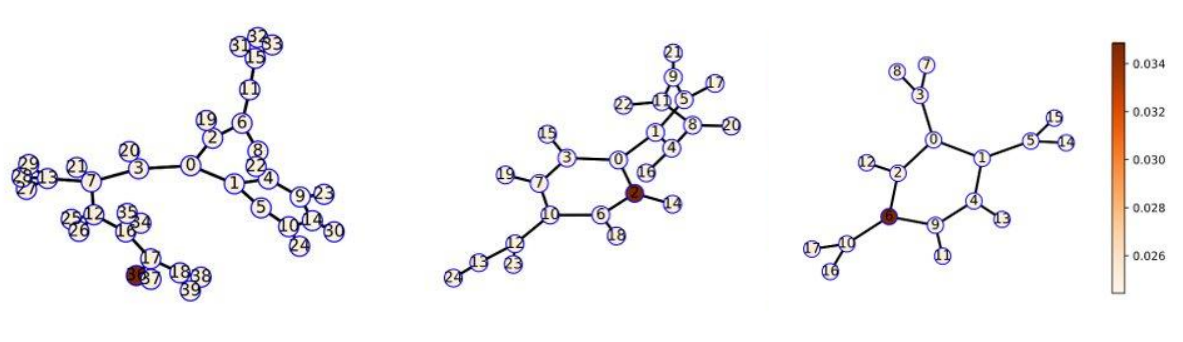
Figure 1 briefly illustrates the working principle of GNNs: the model computes neural message for each node pair and aggregates message for them from their neighbors. A major step of decomposing GNNs is that: the target and background portion of a node are aggregated from the target and background portion of its neighbours, respectively. This can be easily illustrated by the distributive nature of the GNN information aggregation mechanism:

Nevertheless, the above equation is only a conceptual illustration. A real GNN model could consist of various layers, such as graph convolution layers, fully connected layers, activation layers and pooling layers. Several challenges still need to be tackled to develop an effective explanation method. First, how to design the decomposition scheme for different types of layers? Second, how to efficiently find out the important nodes and subgraphs, by choosing the appropriate target/background group given all possible node combinations?

In this work, we consider the decomposition scheme for two commonly used GNN architectures: GCN (Kipf & Welling 2016) and GAT (Veličković et al. 2017).

We first introduce a new scoring function to be used in our algorithm. Different from the absolute contribution scores provided by decomposition, in many scenarios, we are more interested in the relative contribution of the target compared to its contexts. Let $\mathcal{V}^{\gamma}\subset\mathcal{V}$ be the target node group, and $f^{D}(\cdot)$ be the contribution score calculated from decomposition. The relative contribution of $\mathcal{V}^{\gamma}$ averaged over different contexts is calculated as:

where $\mathcal{C}$ is the context around $\mathcal{V}^{\gamma}$, and $\mathcal{N}_{L}\left(\mathcal{V}^{\gamma}\right)$ contains the neighboring nodes of $\mathcal{V}^{\gamma}$ within $L$-hops. Here we use a random walk process $RW()$ to sample $\mathcal{C}$ within the neighborhood around $\mathcal{V}^{\gamma}$. The reason for sampling within the neighborhood is based on the information aggregation, where a node collects the information from its neighbors within certain hops constrained by the GNN depth.

Our agglomeration algorithm initializes from individual nodes and terminates when the whole graph structure is included. Specifically, the interpretation process constructs a series of intermediate subgraph sets $\mathcal{E}=\{\mathcal{S}_{1},...,\mathcal{S}_{I}\}$, where $\mathcal{S}_{i}=\{\mathcal{B}_{1},...,\mathcal{B}_{M_{i}}\}$ contains $M_{i}$ subgraphs. At each step, the algorithm searches for the candidate node or node group $v$ that most significantly affects the contribution of subgraph $\mathcal{B}_{m},m\in\{1,...,M_{i}\}$ according to the ranking score $r(v)$:

where $\mathcal{N}\left(\mathcal{B}_{m}\right)$ is the set of neighbor nodes or node groups to $\mathcal{B}_{m}$. Here $s(v)$ measures the influence of $v$ to $\mathcal{B}_{m}$, while $r(v)$ further revises the value by considering the relative influence of $v$ compared to other candidates $v^{\prime}$. At the beginning of our algorithm, $\mathcal{B}_{m}=\emptyset$. A node $v$ is selected if $r(v)\geq q\cdot\max_{v^{\prime}}r(v^{\prime})$, and we set $q=0.6$ in experiments. The selected nodes are merged into subgraphs to form $\mathcal{S}_{i+1}$. Small subgraphs will be merged into larger ones, so we have $M_{i}\leq M_{j},i\geq j$. The algorithm executes the above steps repeatedly and terminates until all nodes are included (i.e., $M_{i}=1$), or a certain pre-defined step budget is used up. Further details of the algorithm can be found in Section C of the Appendix.

Following the setting in previous work (Ying et al. 2019), we adopt both synthetic datasets and real-world datasets. The statistic of all datasets are given in Sec A in the Appendix.

In this section, we introduce experimental results on both synthetic datasets and the MUTAG dataset. For node classification, the computation graph only contains nodes within $l$-hop from the target node, where $l$ is the number of model layer. The reason is that the nodes outside the computation graph will not influence the final prediction. Table 1 shows the explanation AUC and time efficiency (the training time is shown outside the parentheses for PGExplainer). We have the following key findings. First, DEGREE achieves SOTA performances in most scenarios, showing its advantages in faithfulness over baseline methods. Second, the performance of DEGREE on GCN and GAT models can achieve similar high performance. This observation demonstrates the adaptability of our approach. Third, the improvement of AUC on BA-Community (~9%) and MUTAG (~5%) is more noticeable, where the two datasets distinguish themselves from others is that their features are not constants. It thus shows that our explanation method could well handle node features as they propagate through the graph structure. In terms of efficiency, DEGREE is implemented by decomposing the built-in forward propagation function, so there is no training process. The time cost is highly correlated to the complexity of the target model and the input size. We report further quantitative experiments in Appendix D.

In this section, we use Graph-SST2 and MUTAG datasets to visualize the explanation and demonstrate the effectiveness of our subgraph agglomeration algorithm in Sec 4.

In the first example, we show three visualizations from the MUTAG dataset in Figure 2. The first row represents a correctly predicted instance. Our model successfully identifies the ”NO2” motif as a moderately positive symbol for mutagenicity. The ”H” or the carbon ring is considered a negative sign for mutagenicity. Once the ”NO2” and the ring join, they become a strong positive symbol for mutagenicity. This phenomenon is consistent with the knowledge that the carbon rings and ”NO2” groups tend to be mutagenic (Debnath et al. 1991). We check instances with wrong predictions and show two representative examples. From the second row in Fig. 2, the GCN model precisely finds out the ”NH2” motif with the ring motif as a strong mutagenic symbol. But another wandering part without connection shows a strong non-mutagenic effect, ultimately leading to an incorrect prediction. The second row shows another typical failure pattern. The model catches the ”NH2” and part of the carbon ring as a mutagenic symbol, but the ”CH3” on the bottom right shows a strong non-mutagenic effect. The model erroneously learns a negative interaction between them.

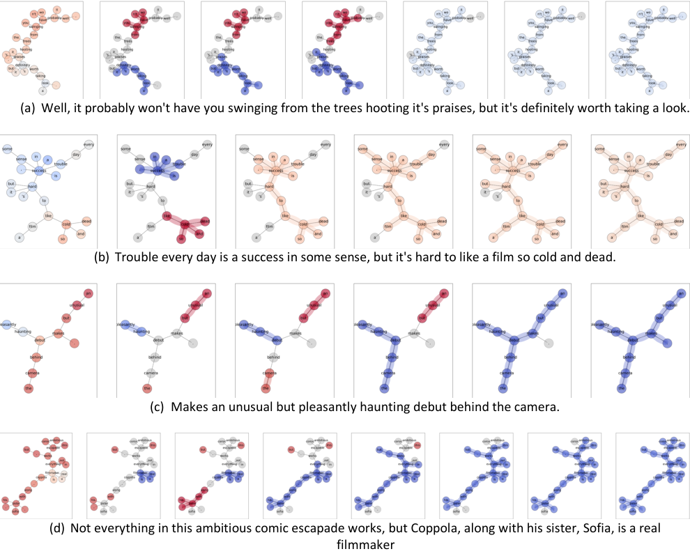
In the second example, we show two visualizations for the Graph-SST2 dataset in Figure 3. The sentence in the first row is labeled negative, yet its prediction is wrong. Our algorithm can explain the decision that the GNN model regards first half of the sentence (”Maybe it’s asking too much”) as negative, the second half (”going to inspire me”, ”want a little more than this”) as positive. But the model can not tell the subjunctive tone behind the word ”if”, and consequently yields a positive but incorrect prediction. The sentence in the second row is negative, and the prediction is correct. Our algorithm precisely identifies the positive part (”Though Ford and Neeson capably hold our interest”) and the negative part (”but its just not a thrilling movie”). Moreover, it reveals that the GCN model can correctly learn the transition relationship between these two components.

We observe that our method can detect non-linear interactions between subgraphs throughout the agglomeration process from above examples. It can help to diagnose the incorrect predictions and enhance the credibility of the model. More visualizations and efficiency study are in Appendix E.

References

- Baldassarre & Azizpour (2019) Federico Baldassarre and Hossein Azizpour. Explainability techniques for graph convolutional networks, 2019.
- Barabási & Albert (1999) Albert-László Barabási and Réka Albert. Emergence of scaling in random networks. science, 286(5439):509–512, 1999.
- Cai & Ji (2020) Lei Cai and Shuiwang Ji. A multi-scale approach for graph link prediction. In Proceedings of the AAAI Conference on Artificial Intelligence, volume 34, pp. 3308–3315, 2020.
- Casas et al. (2019) Sergio Casas, Cole Gulino, Renjie Liao, and Raquel Urtasun. Spatially-aware graph neural networks for relational behavior forecasting from sensor data. arXiv preprint arXiv:1910.08233, 2019.
- Chang et al. (2018) Chun-Hao Chang, Elliot Creager, Anna Goldenberg, and David Duvenaud. Explaining image classifiers by counterfactual generation. arXiv preprint arXiv:1807.08024, 2018.
- Debnath et al. (1991) Asim Kumar Debnath, Rosa L Lopez de Compadre, Gargi Debnath, Alan J Shusterman, and Corwin Hansch. Structure-activity relationship of mutagenic aromatic and heteroaromatic nitro compounds. correlation with molecular orbital energies and hydrophobicity. Journal of medicinal chemistry, 34(2):786–797, 1991.
- Devlin et al. (2019) Jacob Devlin, Ming-Wei Chang, Kenton Lee, and Kristina Toutanova. Bert: Pre-training of deep bidirectional transformers for language understanding, 2019.
- Du et al. (2019) Mengnan Du, Ninghao Liu, and Xia Hu. Techniques for interpretable machine learning. Communications of the ACM, 63(1):68–77, 2019.
- Fan et al. (2019) Wenqi Fan, Yao Ma, Qing Li, Yuan He, Eric Zhao, Jiliang Tang, and Dawei Yin. Graph neural networks for social recommendation. In The World Wide Web Conference, pp. 417–426, 2019.
- Henaff et al. (2015) Mikael Henaff, Joan Bruna, and Yann LeCun. Deep convolutional networks on graph-structured data. arXiv preprint arXiv:1506.05163, 2015.
- Huang et al. (2020) Qiang Huang, Makoto Yamada, Yuan Tian, Dinesh Singh, Dawei Yin, and Yi Chang. Graphlime: Local interpretable model explanations for graph neural networks. arXiv preprint arXiv:2001.06216, 2020.
- Jang et al. (2017) Eric Jang, Shixiang Gu, and Ben Poole. Categorical reparameterization with gumbel-softmax, 2017.
- Kipf & Welling (2016) Thomas N Kipf and Max Welling. Semi-supervised classification with graph convolutional networks. arXiv preprint arXiv:1609.02907, 2016.
- Liang et al. (2020) Jian Liang, Bing Bai, Yuren Cao, Kun Bai, and Fei Wang. Adversarial infidelity learning for model interpretation. In Proceedings of the 26th ACM SIGKDD International Conference on Knowledge Discovery & Data Mining, pp. 286–296, 2020.
- Liu et al. (2020) Cheng-Hao Liu, Maksym Korablyov, Stanisław Jastrzebski, Paweł Włodarczyk-Pruszyński, Yoshua Bengio, and Marwin HS Segler. Retrognn: Approximating retrosynthesis by graph neural networks for de novo drug design. arXiv preprint arXiv:2011.13042, 2020.
- Liu et al. (2021) Meng Liu, Youzhi Luo, Limei Wang, Yaochen Xie, Hao Yuan, Shurui Gui, Haiyang Yu, Zhao Xu, Jingtun Zhang, Yi Liu, Keqiang Yan, Haoran Liu, Cong Fu, Bora Oztekin, Xuan Zhang, and Shuiwang Ji. DIG: A turnkey library for diving into graph deep learning research. arXiv preprint arXiv:2103.12608, 2021.
- Liu et al. (2019) Ninghao Liu, Qiaoyu Tan, Yuening Li, Hongxia Yang, Jingren Zhou, and Xia Hu. Is a single vector enough? exploring node polysemy for network embedding. In Proceedings of the 25th ACM SIGKDD International Conference on Knowledge Discovery & Data Mining, pp. 932–940, 2019.
- Lucic et al. (2021) Ana Lucic, Maartje ter Hoeve, Gabriele Tolomei, Maarten de Rijke, and Fabrizio Silvestri. Cf-gnnexplainer: Counterfactual explanations for graph neural networks, 2021.
- Lundberg & Lee (2017) Scott Lundberg and Su-In Lee. A unified approach to interpreting model predictions, 2017.
- Luo et al. (2020) Dongsheng Luo, Wei Cheng, Dongkuan Xu, Wenchao Yu, Bo Zong, Haifeng Chen, and Xiang Zhang. Parameterized explainer for graph neural network. arXiv preprint arXiv:2011.04573, 2020.
- Murdoch & Szlam (2017) W James Murdoch and Arthur Szlam. Automatic rule extraction from long short term memory networks. arXiv preprint arXiv:1702.02540, 2017.
- Murdoch et al. (2018) W James Murdoch, Peter J Liu, and Bin Yu. Beyond word importance: Contextual decomposition to extract interactions from lstms. arXiv preprint arXiv:1801.05453, 2018.
- Pope et al. (2019) Phillip E Pope, Soheil Kolouri, Mohammad Rostami, Charles E Martin, and Heiko Hoffmann. Explainability methods for graph convolutional neural networks. In Proceedings of the IEEE/CVF Conference on Computer Vision and Pattern Recognition, pp. 10772–10781, 2019.
- Rudin (2019) Cynthia Rudin. Stop explaining black box machine learning models for high stakes decisions and use interpretable models instead. Nature Machine Intelligence, 1(5):206–215, 2019.
- Schnake et al. (2020) Thomas Schnake, Oliver Eberle, Jonas Lederer, Shinichi Nakajima, Kristof T. Schütt, Klaus-Robert Müller, and Grégoire Montavon. Higher-order explanations of graph neural networks via relevant walks, 2020.
- Schwarzenberg et al. (2019) Robert Schwarzenberg, Marc Hübner, David Harbecke, Christoph Alt, and Leonhard Hennig. Layerwise relevance visualization in convolutional text graph classifiers, 2019.
- Shrikumar et al. (2017) Avanti Shrikumar, Peyton Greenside, and Anshul Kundaje. Learning important features through propagating activation differences. In International Conference on Machine Learning, pp. 3145–3153. PMLR, 2017.
- Simonyan et al. (2013) Karen Simonyan, Andrea Vedaldi, and Andrew Zisserman. Deep inside convolutional networks: Visualising image classification models and saliency maps. arXiv preprint arXiv:1312.6034, 2013.
- Singh et al. (2018) Chandan Singh, W James Murdoch, and Bin Yu. Hierarchical interpretations for neural network predictions. arXiv preprint arXiv:1806.05337, 2018.
- Sundararajan et al. (2017) Mukund Sundararajan, Ankur Taly, and Qiqi Yan. Axiomatic attribution for deep networks. In International Conference on Machine Learning, pp. 3319–3328. PMLR, 2017.
- Veličković et al. (2017) Petar Veličković, Guillem Cucurull, Arantxa Casanova, Adriana Romero, Pietro Lio, and Yoshua Bengio. Graph attention networks. arXiv preprint arXiv:1710.10903, 2017.
- Vu & Thai (2020) Minh N Vu and My T Thai. Pgm-explainer: Probabilistic graphical model explanations for graph neural networks. arXiv preprint arXiv:2010.05788, 2020.
- Wang et al. (2021) Xiang Wang, Yingxin Wu, An Zhang, Xiangnan He, and Tat seng Chua. Causal screening to interpret graph neural networks, 2021. URL https://openreview.net/forum?id=nzKv5vxZfge.
- Xu et al. (2018) Keyulu Xu, Weihua Hu, Jure Leskovec, and Stefanie Jegelka. How powerful are graph neural networks? arXiv preprint arXiv:1810.00826, 2018.
- Ying et al. (2019) Rex Ying, Dylan Bourgeois, Jiaxuan You, Marinka Zitnik, and Jure Leskovec. Gnnexplainer: Generating explanations for graph neural networks. Advances in neural information processing systems, 32:9240, 2019.
- Yuan et al. (2020) Hao Yuan, Jiliang Tang, Xia Hu, and Shuiwang Ji. Xgnn: Towards model-level explanations of graph neural networks. In Proceedings of the 26th ACM SIGKDD International Conference on Knowledge Discovery & Data Mining, pp. 430–438, 2020.
- Yuan et al. (2021) Hao Yuan, Haiyang Yu, Jie Wang, Kang Li, and Shuiwang Ji. On explainability of graph neural networks via subgraph explorations. arXiv preprint arXiv:2102.05152, 2021.
- Zhang & Chen (2018) Muhan Zhang and Yixin Chen. Link prediction based on graph neural networks. arXiv preprint arXiv:1802.09691, 2018.
- Zhang et al. (2018) Muhan Zhang, Zhicheng Cui, Marion Neumann, and Yixin Chen. An end-to-end deep learning architecture for graph classification. In Proceedings of the AAAI Conference on Artificial Intelligence, volume 32, 2018.
- Zhou et al. (2018) Jie Zhou, Ganqu Cui, Zhengyan Zhang, Cheng Yang, Zhiyuan Liu, Lifeng Wang, Changcheng Li, and Maosong Sun. Graph neural networks: A review of methods and applications. arXiv preprint arXiv:1812.08434, 2018.
Appendix A Datasets and Experimental Setting
In this section, we introduce the detail of the datasets as wall as the experimental setting. The code can be found at https://anonymous.4open.science/r/DEGREE-3128.
Model setup: We adopt GCN model and GAT model architecture for corresponding experiments. We use to denote a GCN layer, and similar notation for GAT layer and fully connected layer.
The structure of GCN model for node classification task is following:
.
For graph classification task, we adopt a Max-pooling layer before the FC layers:
For GAT model architecture, we replace all GCN layers with GAT layer and keep the remaining setting unchanged. For experiments on Tree-Grid dataset, we adopt 4-layer GCN/GAT model by adding one more GCN/GAT layer with same setting before FC layers.
Dataset statistic: The statistics of synthetic datasets and real-world datasets are reported in Table 2.