Combinatorial-hybrid Optimization for Multi-agent Systems
under Collaborative Tasks

The first layer assigns the set of tasks to available agents. To begin with, the task assignment problem is formulated based on the literature of coalition formation [26, 27]. Particularly, consider the coalition structure defined as follows:

where $\mathcal{R}=\{1,\cdots,N\}$ is the team of $N$ agents; $\Omega=\{\omega_{1},\cdots,\omega_{M}\}$ is the set of $M$ tasks; $f:2^{\mathcal{R}}\times\Omega\rightarrow\mathbb{R}^{+}$ is the cost function of a potential coalition for any given task in $\Omega$. Not that since the exact cost $f$ above is often unknown, thus estimated initially by simple heuristics such as Euclidean distance, denoted by $\widehat{f}$.

Let $\mu(\omega_{m})=\mathcal{R}_{m}$ return the coalition for task $\omega_{m}$ and $\mu(n)=\omega_{m}$ return the task assigned to agent $n$, $\forall n\in\mathcal{R}_{m}$. More importantly, an assignment $\mu$ can be modified via the following switch operation.

Given the above definitions, the first layer of coalition formation is transformed into the problem of finding a Nash-stable assignment as follows.

The proposed solution follows an iterative switching operations to reduce the largest cost of all tasks. An initial assignment $\mu_{0}$ can be derived in a random or greedy way. Then, the target coalition with the $k$-th maximum cost is selected via:

where $k=1$ initially for the maximum cost; and ties are broken arbitrarily. Given $(\mathcal{R}_{m^{\star}},\omega_{m^{\star}})$, the first step is to calculate the actual utility $f_{m^{\star}}$, via the hybrid optimization procedure described in the subsequent section. There are two possible outcomes: (I) If $f_{m^{\star}}\geq\textbf{max}_{m\neq m^{\star}}\{\widehat{f}_{m}\}$, it means that $\omega_{m^{\star}}$ remains the target coalition. As illustrated in Fig. 3, the goal is to find a switch operation $\sigma^{m^{\star}}_{n}$ for one agent $n\in\mathcal{N}$ such that after applying $\sigma^{m^{\star}}_{n}$ the maximum cost is reduced, i.e.,

where $m^{-}=\mu_{0}(n)$ is the task to which agent $n$ was assigned before applying the switch. Such a switch can be found by iterating through all agents within $\mathcal{R}\backslash\mathcal{R}_{m^{\star}}$, and verifying whether the condition in (10) holds. Once a switch $\sigma^{m^{\star}}_{n}$ is found, a new assignment is given by $\mu_{1}=\sigma^{m^{\star}}_{n}(\mu_{0})$, after which a new target coalition can be found via (9). (II) If $f_{m^{\star}}<\textbf{max}_{m\neq m^{\star}}\{\widehat{f}_{m}\}$, it means that $\omega_{m^{\star}}$ is no longer the target coalition based on its actual cost. Then, the estimated utility $\widehat{f}_{m^{\star}}$ is updated accordingly and thus a new target coalition can be found via (9). The above procedure is repeated until the target coalition does not change anymore, of which the assignment and target coalition are denoted by $\mu_{K_{1}}$ and $(\omega_{m_{1}^{\star}},\mathcal{R}_{m_{1}^{\star}})$, respectively.

Afterwards, the same process is repeated but focusing on the target coalition with second largest cost, i.e., by setting $\mu_{K_{1}}$ as the initial assignment and $k=2$ instead in (9). Similarly, the procedure converges in this round after the target coalition remains unchanged. The same round is performed for $k=3$ and so on until $k=M$, when the target coalition $\mu_{K_{M}}$ has the minimum utility. Note that if the target coalitions from the previous rounds, e.g., round $k_{1}$, are changed during the current round $k_{2}>k_{1}$, the whole process is re-started from $k=1$.

For the ease of notation, let $\mathbf{X}=x_{k_{0}^{m}}\cdots x_{k_{T}^{m}}$ be the sequence of system states at discrete time steps $t=0,1,\cdots,T$ for a sufficient duration $T$; $\mathbf{\Xi}=\xi_{k_{t_{1}}^{m}},\cdots,\xi_{k_{t_{N}}^{m}}$ and $\mathbf{P}=\rho_{k_{t_{1}}^{m}},\cdots,\rho_{k_{t_{N}}^{m}}$ be the sequence of modes applied to the system for time periods $[t_{0},t_{1}),\,[t_{1},t_{2}),\,\cdots,\,[t_{N-1},t_{N})$, where $t_{n}=nT_{0},T_{0}\in\mathbb{N}$, $\forall n=0,\cdots,\lfloor\frac{T}{T_{0}}\rfloor$. Note that $T_{0}>0$ is chosen as a lower bound on the duration of each mode to avoid too frequent switching of modes and parameters. Furthermore, let $\mathbf{X}_{t},\,\mathbf{\Xi}_{t},\,\mathbf{P}_{t}$ denote $x_{k_{t}^{m}},\,\xi_{k_{t}^{m}},\,\rho_{k_{t}^{m}}$. Then, the hybrid optimization problem is stated as follows:

Note that different from the original combinatorial-hybrid optimization problem in (6), the goal of the hybrid optimization problem above is to find the optimal hybrid plan $\varphi_{m}$ for a specific task $\omega_{m}$ and the corresponding coalition $\mathcal{R}_{m}$. A novel hybrid-search algorithm called Heuristic Gradient-Guided Hybrid Search (HGG-HS) is proposed to solve Problem 3. Instead of feeding the above problem directly into a general nonlinear optimizer, the proposed algorithm combines: (i) the $A^{\star}$-based discrete search for the optimal sequence of modes, and (ii) the gradient-based optimization for the optimal sequence of parameters. More specifically, the hybrid search tree is defined as $\mathcal{T}\triangleq(V,\,E,\,\nu_{0},\,V_{G})$, where $V=\{\nu\}$ is a set of vertices for $\nu\in\mathcal{X}_{\texttt{safe}}$; $E\subset V\times V$ is a set of edges; $\nu_{0}\in V$ is the initial vertex; and $V_{G}\subset V$ is a set of goal states determined by $\mathcal{X}_{G_{m}}$. Moreover, let $cost(\nu)$ be the cost of node $\nu$ and $prev(\nu)$ be the parent node of $\nu$.

As stated in [28], a proper design of the heuristic function $h:\mathcal{X}\rightarrow\mathbb{R}^{+}$ is essential for the performance of the $A^{\star}$ search algorithm. Since it is impractical to find an exact heuristic function $h^{\texttt{opt}}$ that estimates perfectly the cost from a given vertex $\nu\in V$ to the goal set $V_{G}$, this work proposes two approximations of the exact heuristics at different level of abstraction: (i) the global approximation $h^{\mathcal{G}}$ that serves as a lower bound on the actual cost, i.e., $h^{\texttt{opt}}(x)\geq h^{\mathcal{G}}(x)$, $\forall x\in\mathcal{X}$. For instance, Euclidean distance is a common choice as admissible heuristics; (ii) the local approximation $h^{\mathcal{L}}$ that is differentiable and has similar gradients to $h^{\texttt{opt}}$ in a local neighborhood, i.e., $\|\nabla h^{\mathcal{L}}_{x_{0}}(x)-\nabla h^{\texttt{opt}}(x)\|\leq E$, $\forall x\in\mathrm{U}_{d}(x_{0})=\{x\in\mathcal{X}|\|x-x_{0}\|\leq d\}$ and $E>0$. Furthermore, a balanced heuristic function $h^{\mathcal{B}}$ is defined recursively as follows:

where $\tilde{\nu}=prev(\nu)$; $\lambda\in[0,1]$ is a weighting factor; and $\Delta h(\tilde{\nu},\,\nu)$ is the change of cost from $\tilde{\nu}$ to $\nu$, which is estimated by the accumulated change along a path, i.e.,

where $x_{0}=\tilde{\nu}$, $x_{L}=\nu$, and $x_{\ell}\in\mathrm{U}_{d}(x_{\ell-1})$, $\forall\ell=1,\cdots,L$. Moreover, $\lambda$ is a parameter that effects the greedy-ness of HGG-HS. Namely, when $\lambda=0$ holds, $h^{\mathcal{B}}$ reduces to $h^{\mathcal{G}}$, yielding a general heuristic search algorithm like $A^{\star}$. On the other hand, when $\lambda=1$ holds, $h^{\mathcal{B}}$ only depends on the local approximation $h^{\mathcal{L}}$, resulting in a local greedy search.

Given the above definition of balanced heuristics, the hybrid search tree $\mathcal{T}$ is explored via an iterative process of node selection and expansion. To begin with, similar to the $A^{\star}$ algorithm, a priority queue $V_{\texttt{op}}\subset V$ is used to store the vertices to be visited, while a set $V_{\texttt{cl}}\subset V$ is used to store the vertices that have been fully explored. Then, as illustrated in Fig. 4, the proposed hybrid search algorithm consists of the following stages: (I) Selection. The vertex with the lowest estimated cost in $V_{\texttt{op}}$ is selected, i.e., $\nu^{\star}=\textbf{argmin}_{\nu\in V_{\texttt{op}}}\{cost(\nu)+h^{\mathcal{B}}(\nu)\}$, of which the associated state is $x^{\star}$. (II) Expansion. This vertex $\nu^{\star}$ is expanded in three steps: (i) first, a feasible mode $\xi\in\Xi$ is chosen given the state $x^{\star}$; (ii) then, a set of candidate parameters $\{\rho^{\star}\}\subset\mathcal{P}_{\xi}$ is found for mode $\xi$ and $x^{\star}$ via an iterative optimization in the parameter space as described in the sequel; (iii) lastly, given $\xi$ and $\{\rho^{\star}\}$ above, the set of resulting child vertices $\mathcal{C}_{\xi}(\nu^{\star})\triangleq\{\nu^{+}\}$ is given by:

which is encapsulated by $\nu^{+}\triangleq\texttt{Expand}(x^{\star},\,\rho^{\star})$ for the ease of notation. Moreover, the properties of $\nu^{+}$ is updated by $cost(\nu^{+})=cost(\nu^{\star})+\sum_{t=0}^{T_{0}}c_{\text{cont}}(\mathbf{x}_{t},\,\rho^{\star})$ and $prev(\nu^{+})=\nu^{\star}$. Each child node $\nu^{+}\in\mathcal{C}_{\xi}(\nu^{\star})$ is added to the node set $V$ and $V_{\texttt{op}}$, if $\nu\notin V_{\texttt{cl}}$ and $cost(\nu^{+})\leq cost(\nu)$, $\forall\nu\in V$ that satisfying $[(\nu^{+}-\nu)/\delta]=\mathbf{0}$, where $[\cdot]$ is the rounding function for a radius $\delta>0$. Afterwards, the edge $(\nu^{\star},\nu^{+})$ is added to the edge set $E$ and labeled by the associated mode and parameter $(\xi,\,\rho^{\star})$. (III) Termination. If all the child vertices of $\nu^{\star}$ have been explored, $\nu^{\star}$ is removed from $V_{\texttt{op}}$ and added to $V_{\texttt{cl}}$. More importantly, if $\nu^{\star}\in V_{G}$ holds, the optimized sequences $\mathbf{\Xi}$ and $\mathbf{P}$ as the solution to Problem 3 can be obtained by tracing back the parent vertices and retrieving its label $(\xi,\,\rho)$. Thus, the hybrid search algorithm returns the hybrid plan as described in (11), along with the actual cost for the assigned task.

The optimization for parameter $\rho^{\star}$ in the stage of expansion above for node $\nu^{\star}$ follows a two-stage process. In the first stage of primitive expansion, parameters are initially selected from a predefined set of primitive parameters $\{\hat{\rho}_{1},\cdots,\hat{\rho}_{I}\}\subset\mathcal{P}_{\xi}$. Then, a set of child vertices can be generated by $\nu_{i}^{+}=\texttt{Expand}(x^{\star},\,\hat{\rho}_{i})$, $\forall\hat{\rho}_{i}\in\hat{\mathcal{P}}_{\xi}$. Within this set, the child vertex with lowest estimated total cost is selected, i.e.,

and the associated parameter is $\hat{\rho}_{i^{\star}}$. In the second stage of iterative optimization, the end state $x_{\texttt{e}}^{(\ell)}$ and the associated parameter $\rho^{(\ell)}$ is optimized via nonlinear optimization for iterations $\ell=1,\cdots,L$. Initially, $x_{\texttt{e}}^{(0)}=\nu_{i^{\star}}$ and $\rho^{(0)}=\hat{\rho}_{i^{\star}}$. Then, the following procedure is applied to update $\rho^{(\ell)}$:

which can be solved by a general nonlinear optimization solver such as IPOPT [29], as all states are parameterized over $\rho$. Once $\rho^{(\ell+1)}$ is obtained, the associated end state is updated by $x^{(\ell+1)}_{\texttt{e}}=\texttt{Expand}(\nu^{\star},\,\rho^{(\ell+1)})$. This iterative process continues until iteration $L$ such that $\|x^{(L)}_{\texttt{e}}-x^{(L-1)}_{\texttt{e}}\|<d$. Consequently, the set of pairs of parameters and end states is given by $\{(\rho^{(\ell)},\,x^{(\ell)}_{\texttt{e}})\}$, of which the corresponding child vertices are $\{\nu^{+}_{(\ell)}\}$. Thus, the set of all child vertices $\mathcal{C}_{\xi}(\nu^{\star})=\{\nu^{+}_{i},\forall i\}\cup\{\nu^{+}_{(\ell)},\forall\ell\}$ is sent to the next step in the stage of expansion.

As introduced in Sec. III-A and shown in Fig. 5, the workspace of size $10m\times 10m$ is cluttered with rectangular obstacles. There are $16$ agents and $6$ boxes randomly distributed within the workspace. Each box has a size of $1m\times 0.5m$, and the circular agents have a radius $r=0.1m$. For simplicity, each robot has a first-order dynamics and can provide bounded pushing force at specific points of the box, thus changing the state of boxes with second-order translational invariant dynamics. Note that the cluttered workspace introduces severe geometric constraints, yielding a significantly more difficult transportation task than the obstacle-free environments [19, 20]. Initially, the task cost $f(\cdot)$ in (7) is estimated by the sum of Euclidean distances from agents to the targeted box, and the distance to its goal position. The heuristic function $h^{\mathcal{G}}(x)$ is designed as the minimum distance from state $x$ to $\mathcal{X}_{G_{m}}$, estimated by the $A^{\star}$ search, and $h^{\mathcal{L}}(x)$ is designed as the kinematic cost under the local geometry constraints from current state $x$ to next intermediate region $\hat{\mathcal{X}}$ on the shortest path.

Evolution of the system state is shown in Fig. 5. Initially, the coalition formation for $6$ tasks and $16$ agents takes $9s$, during which $16$ hybrid search problems are solved in the hybrid optimization layer. It can be seen that different modes have a significant influence on overall cost. e.g., box $5$ reaches its goal location faster by choosing a short-side pushing mode with $2$ agents to pass through a narrow passage; $3$ agents are assigned to box $4$ such that it can be pushed through $2$ passages that are far away; box $5$ is pushed to its target by $4$ agents via almost a straight line. To further validate the applicability, another complex scenario is considered and shown in Fig. 5, where numerous sharp turns are required for the boxes to arrive at the destinations. Consequently, more frequent mode switchings can be found in the final solution, e.g., the coalition of $4$ agents associated with box $3$ switches the mode from the “long side” to the “short side”, such that the box could pass through the first passage at $t=45s$. However, since pushing from a narrow side introduces higher kinematic uncertainty and thus larger cost, the same coalition switches to the “diagonally pushing” mode after passing through the second passage at $t=92s$. Furthermore, for both boxes $1$ and $2$, two agents switch from “long-side” to “short-side” for the middle passage at $t=70$.

As introduced in Sec. III-B and shown in Fig. 6, the workspace contains randomly placed obstacles of various shapes like corridors and corners, yielding a much more difficult capture task than the obstacle-free environments [3, 24]. There are $10$ pursuers and $3$ evaders randomly distributed in a workspace of size $2.5m\times 2.5m$. For simplicity, all agents satisfy the single-integrator dynamics, with the same maximum velocity of $4m/s$. The system state is available at all time for the pursuers. The capture radius of pursuers is set to $0.15m$. As described in Sec. III-B, the pursuers follow three parameterized modes to capture the evaders in a collaborative way. The task cost $f(\cdot)$ in (7) is estimated by the weighted average distance from the pursuers in a coalition to the assigned evader. Heuristics $h^{\mathcal{G}}(\cdot)$ is designed as the minimum distance to the evader, and $h^{\mathcal{L}}(\cdot)$ is designed according to specific local environments, e.g.,the area of the corner envelop for enclosure mode. Lastly, the parameter associated with mode of “pure pursuit” is determined solely by the position of the targeted evader; the parameter for the mode of “hide and attack” is sampled from a set of potential locations given the workspace layout and the targeted evader; the parameter for the mode of “enclosure” is determined by maximizing the region of advantage [25].

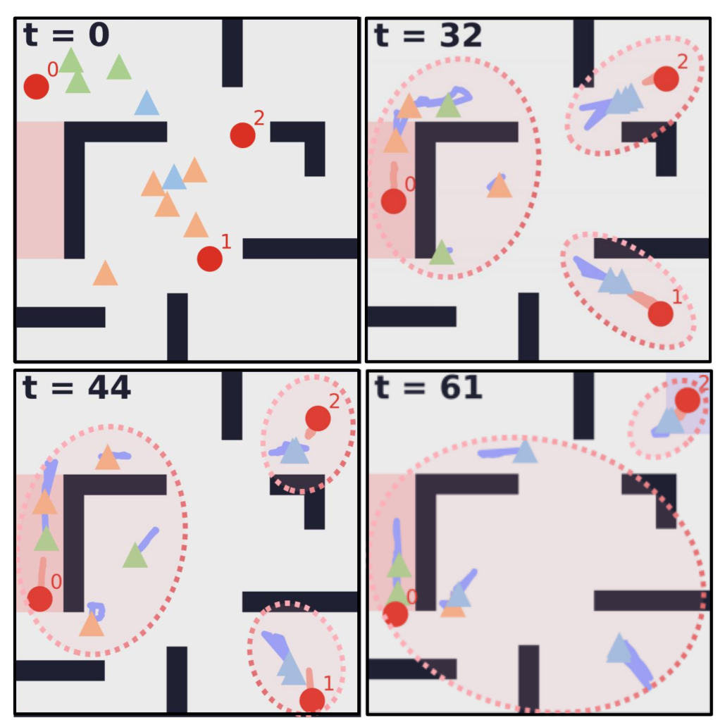
The first layer of task allocation process is executed every $15$ time steps, while the layer of hybrid optimization is updated every $5$ time steps to adapt to the fast movement of evaders. Evolution of the system under one solution is visualized in Fig. 6. Initially, the position of pursuers and evaders are initialized randomly. As shown in Fig. 7, pursers $0,1,2,3$ and $6$ are assigned to capture evader $0$ initially, while pursers $4,5$ for evader $1$, and pursers $7,8,9$ for evader $2$. At $t=50$, evader $1$ is captured under the mode “enclosure” by setting the parameters as even dividers on the boundary of advantage region. Afterwards, pursuers $4,5$ join the coalition for evader $2$ with the mode “pure pursuit”. Then, evader $2$ is captured at $t=69$ under the mode “enclosure”, after which pursuers $4,5$ join the coalition for evader $0$ with the mode “hide and attack”. It can be seen that the selected parameters for this mode are mainly located around the four corners of obstacles in the middle. All evaders are captured at $t=75$, during which there are in total $3$ switches of tasks and $24$ switches of modes.

References

- [1] T. Bock, “Construction robotics,” Autonomous Robots, vol. 22, no. 3, pp. 201–209, 2007.
- [2] M. Krizmancic, B. Arbanas, T. Petrovic, F. Petric, and S. Bogdan, “Cooperative aerial-ground multi-robot system for automated construction tasks,” IEEE Robotics and Automation Letters, vol. 5, no. 2, pp. 798–805, 2020.
- [3] A. Pierson, Z. Wang, and M. Schwager, “Intercepting rogue robots: An algorithm for capturing multiple evaders with multiple pursuers,” IEEE Robotics and Automation Letters, vol. 2, no. 2, pp. 530–537, 2016.
- [4] A. Khan, B. Rinner, and A. Cavallaro, “Cooperative robots to observe moving targets,” IEEE transactions on cybernetics, vol. 48, no. 1, pp. 187–198, 2016.
- [5] A. Torreño, E. Onaindia, A. Komenda, and M. Štolba, “Cooperative multi-agent planning: A survey,” ACM Computing Surveys (CSUR), vol. 50, no. 6, pp. 1–32, 2017.
- [6] M. Gini, “Multi-robot allocation of tasks with temporal and ordering constraints,” in AAAI Conference on Artificial Intelligence, 2017.
- [7] R. Massin, C. J. Le Martret, and P. Ciblat, “A coalition formation game for distributed node clustering in mobile ad hoc networks,” IEEE Transactions on Wireless Communications, vol. 16, no. 6, pp. 3940–3952, 2017.
- [8] I. E. Weintraub, M. Pachter, and E. Garcia, “An introduction to pursuit-evasion differential games,” in IEEE American Control Conference (ACC), 2020, pp. 1049–1066.
- [9] J. Tordesillas and J. P. How, “Mader: Trajectory planner in multiagent and dynamic environments,” IEEE Transactions on Robotics, vol. 38, no. 1, pp. 463–476, 2021.
- [10] V. R. Makkapati and P. Tsiotras, “Optimal evading strategies and task allocation in multi-player pursuit-evasion problems,” Dynamic Games and Applications, vol. 9, pp. 1168–1187, 2019.
- [11] V. N. Hartmann, O. S. Oguz, D. Driess, M. Toussaint, and A. Menges, “Robust task and motion planning for long-horizon architectural construction planning,” in IEEE/RSJ International Conference on Intelligent Robots and Systems (IROS), 2020, pp. 6886–6893.
- [12] A. Khamis, A. Hussein, and A. Elmogy, “Multi-robot task allocation: A review of the state-of-the-art,” Cooperative Robots and Sensor Networks 2015, pp. 31–51, 2015.
- [13] R. Fukasawa, H. Longo, J. Lysgaard, M. P. De Aragão, M. Reis, E. Uchoa, and R. F. Werneck, “Robust branch-and-cut-and-price for the capacitated vehicle routing problem,” Mathematical programming, vol. 106, no. 3, pp. 491–511, 2006.
- [14] E. Nunes and M. Gini, “Multi-robot auctions for allocation of tasks with temporal constraints,” in AAAI Conference on Artificial Intelligence, vol. 29, no. 1, 2015.
- [15] R. Jonker and T. Volgenant, “Improving the hungarian assignment algorithm,” Operations Research Letters, vol. 5, no. 4, pp. 171–175, 1986.
- [16] K. R. Apt and A. Witzel, “A generic approach to coalition formation,” International game theory review, vol. 11, no. 03, pp. 347–367, 2009.
- [17] E. Soria, F. Schiano, and D. Floreano, “Distributed predictive drone swarms in cluttered environments,” IEEE Robotics and Automation Letters, vol. 7, no. 1, pp. 73–80, 2021.
- [18] X. Sun and C. G. Cassandras, “Optimal dynamic formation control of multi-agent systems in constrained environments,” Automatica, vol. 73, pp. 169–179, 2016.
- [19] E. Tuci, M. H. Alkilabi, and O. Akanyeti, “Cooperative object transport in multi-robot systems: A review of the state-of-the-art,” Frontiers in Robotics and AI, vol. 5, p. 59, 2018.
- [20] K. I. Alevizos, C. P. Bechlioulis, and K. J. Kyriakopoulos, “Bounded energy collisions in human–robot cooperative transportation,” IEEE/ASME Transactions on Mechatronics, vol. 27, no. 6, pp. 4541–4549, 2022.
- [21] M. Guo, J. Tumova, and D. V. Dimarogonas, “Communication-free multi-agent control under local temporal tasks and relative-distance constraints,” IEEE Transactions on Automatic Control, vol. 61, no. 12, pp. 3948–3962, 2016.
- [22] M. Guo and M. M. Zavlanos, “Multirobot data gathering under buffer constraints and intermittent communication,” IEEE transactions on robotics, vol. 34, no. 4, pp. 1082–1097, 2018.
- [23] M. Dogar, A. Spielberg, S. Baker, and D. Rus, “Multi-robot grasp planning for sequential assembly operations,” Autonomous Robots, vol. 43, pp. 649–664, 2019.
- [24] M. Chen, Z. Zhou, and C. J. Tomlin, “Multiplayer reach-avoid games via pairwise outcomes,” IEEE Transactions on Automatic Control, vol. 62, no. 3, pp. 1451–1457, 2016.
- [25] A. Von Moll, D. W. Casbeer, E. Garcia, and D. Milutinović, “Pursuit-evasion of an evader by multiple pursuers,” in International Conference on Unmanned Aircraft Systems (ICUAS), 2018, pp. 133–142.
- [26] T. Rahwan, T. P. Michalak, M. Wooldridge, and N. R. Jennings, “Coalition structure generation: A survey,” Artificial Intelligence, vol. 229, pp. 139–174, 2015.
- [27] Q. Li, M. Li, B. Q. Vo, and R. Kowalczyk, “An anytime algorithm for large-scale heterogeneous task allocation,” in International Conference on Engineering of Complex Computer Systems (ICECCS), 2020, pp. 206–215.
- [28] S. Cui, X. Jin, S. Wang, Y. He, and Q. Huang, “Heuristic domain adaptation,” Advances in Neural Information Processing Systems, vol. 33, pp. 7571–7583, 2020.
- [29] A. Wächter, “Short tutorial: Getting started with ipopt in 90 minutes,” in Dagstuhl Seminar Proceedings. Schloss Dagstuhl-Leibniz-Zentrum fuer Informatik, 2009.