High Dimensional Geometry and Limitations in System Identification
Abstract
We study the problem of identification of linear dynamical system from a single trajectory, via excitations of isotropic Gaussian. In stark contrast with previously reported results, Ordinary Least Squares (OLS) estimator for even stable dynamical system contains non-vanishing error in high dimensions; which stems from the fact that realizations of non-diagonalizable dynamics can have strong spatial correlations and a variance, of order , where is the dimension of the underlying state space. Employing concentration of measure phenomenon, in particular tensorization of Talagrands inequality for random dynamical systems we show that observed trajectory of dynamical system of length- can have a variance of order . Consequently, showing some or most of the distances between an dimensional random vector and an dimensional hyperplane in can be close to zero with positive probability and these estimates become stronger in high dimensions and more iterations via Isoperimetry. Negative second moment identity, along with distance estimates give a control on all the singular values of Random matrix of data, revealing limitations of OLS for stable non-diagonalizable and explosive diagonalizable systems.
1 Introduction
The task of estimating parameters associated to an unknown dynamical systems is of fundamental importance in finance, econometrics, controls and reinforcement learning. Last decade has seen a tremendous surge in research work on finite-time analysis on learning for dynamical systems. In this work we demystify the working of OLS estimator for dynamical system , i.e., estimating state transition matrix by using excitations of isotropic Gaussian and observed trajectory . Understanding this problem is causal for dealing with more involved problems like learning dynamics from input-output data (Oymak and Ozay 2021) and online Kalman filtering (Tsiamis and Pappas 2022). In contrast with existing results Sarkar et al. 2019; Simchowitz et al. 2018; Faradonbeh et al. 2018; Faradonbeh et al. 2018 which only seems to work via careful selection of spectrum of state transition matrix and length of simulated trajectory and scalar systems, our analysis is particularly focused towards high dimensional state space. To the best of authors’ knowledge we give first geometric analysis for system identification by leveraging upon recent developments in random matrix theory literature Tao et al. 2010; Tao 2012; Vu 2014; Rudelson and Vershynin 2009 and direct sum decomposition of original state transition matrix onto its’ invariant subspaces for non-diagonalizable systems. Indeed these invariant subspaces correspond to Jordan forms but standard results in literature only focus on algebraic properties of Jordan forms, ignoring the hidden geometric content. Along with Talagrand’s concentration inequality we are able to conclude, as opposed to standard beliefs, main issue in system identification and for stable systems is strong spatial correlations: that stem from existence of invariant subspaces of large dimensions, Naeem 2023. Large invariant subspaces are a consequence of discrepancy between algebraic and geometric multiplicity of eigenvalues associated to state transition matrix, leading to recursive generation of basis that naturally add spatial correlations.
Contributions and main results:
In this paper we show that analysis based on mere magnitude of eigenvalues associated to state transition is misleading as non-hermitian matrices naturally contain important geometric content that can not be taken for granted. Our analysis is based in Frobenius norm which is sensitive to all the modes rather than the most dominant one, as small error in operator norm can be misleading. We have been wasteful with some of the concentration results, as our aim is to make things interpretable and accessible to general machine learning community. If the observed trajectory is , the trick is to understand the geometry of its rows . Consider the row and the hyperplane spanned by all rows modulo , error increases as soon as any of these distances become small. In the case of diagonalizable dynamics this is the case when their is an explosive mode; as it can have large variance and with decent probability be close to a high dimensional random subspace. Non-diagonalizable stable dynamics are naturally correlated in space, and in higher dimensions with increase in iterations their variance and largest singular value increases exponentially.
Structure of the paper:
We begin section 2 with notations, followed by important results from concentration of measure phenomenon for random dynamical systems. In Section 3, we formally define the OLS problem and provide a very’ detailed analysis on Diagonalizable systems, as it will simplify understanding for non-hermitaian dynamics. Section 4 begins with geometric analysis of non-diagonalizable matrices and limitations of OLS are verified via simulation results. We conclude our analysis in Section 5, with conclusions and directions on future work.
2 Concentration of measure phenomenon for random dynamical systems
Notations:
We use to denote the dimensional identity matrix. For random variables and , denote the correlation/covariance. , is the unit sphere in . Whereas, , , , , , and represent the transpose, spectral radius, matrix 2-norm (operator norm) , Frobenius norm, determinant, trace and set of eigenvalues(spectrum) of respectively. , and are standard order relations. For a positive definite matrix , largest and smallest eigenvaues are denoted by and , respectively. Associated with every rectangular matrix are its’ singular values , where without loss of generality we assume that . More frequently used are the largest singular value, and the smallest singular value . Condition number of a matrix is the ratio of the largest and least singular value, denoted by . If the span of image space of is , more compactly written as , least singular value equals the inverse of the norm of inverse of matrix i.e., . A function is Lipschitz with constant if for every , . Space of probability measure on (continuous space) is denoted by and space of its Borel subsets is represented by . For a function and , we use to denote expectation of w.r.t .On a metric space , for , we define Wasserstein metric of order as
| (1) |
here, , and implies that random variables follow some probability distributions on with marginals and . Another way of comparing two probability distributions on is via relative entropy, which is defined as
| (2) |
Notions of stability:
Markov chain under consideration is dimensional LG with isotropic noise:
| (3) |
It mixes to stationary distribution , where the controllability grammian is the unique positive definite solution of the following Lyapunov equation:
| (4) |
Stability in controls community for Linear systems correspond to (marginally stable corresponds and explosive system when )
Definition 2.1 (Talagrands inequality).
Consider metric space and reference probability measure . Then we say that satisfies or to be concise for some if for all it holds that
| (5) |
Theorem 2.2.
If satisfies then for all Lipschitz function with , it holds that
| (6) |
Moreover, (6) combined with the Markov inequality implies that if we sample from , then
| (7) |
Since we will be dealing with the dependent processes, it is important to understand the concentration phenomenon for the entire length of simulated trajectory, a tensorization procedure for Talagrands inequality is required. If one is concerned with the concentration of time averages around steady state spatial average, as in Naeem and Pajic 2022 an based metric suffices. However, when dealing with projections and distances in large dimension, following metric on product space is more appropriate with associated variance constants.
Theorem 2.3.
[Tensorization of Talagrands’ Inequality for Dependent Processes] Let, be an inspired metric on . If system transition matrix, for LG satisfies , then the process level law of satisfies , if we have and for , Blower and Bolley 2005.
A fundamental limitation of existing results, stem from the fact that they base their analysis only on the extreme singular values of the data matrix which do not offer much of geometric insight. This brings us to an extremely important, although simple to prove equality that relates the distance between different rows (whose concentration we understand well because of preceding theorem 2.3) of the data matrix to all of its’ singular values.
Theorem 2.4.
Tao et al. 2010 [Negative second moment identity ] Let and be a full rank matrix with singular values, . Let be the hyperplane generated by all the rows of -except the : i.e., span of for and be the canonical basis of
| (8) |
As the quantifying distance between a subspace and vector involves taking projections, high probability estimates will require concentration behavior of projections of isotropic Gaussians, as in:
Theorem 2.5.
[Gaussian Projection and Isoperimetry, Lemma 3.2 in Barvinok 2005] Let be isotropic Gaussian in and be a dimensional subspace. Given , let denote the projection of onto . Then for any
| (9) |
and we will often denote this behavior as or say with overwhelming probability
3 Problem statement: system Identification via single trajectory
3.1 Ordinary Least Squares estimator
In this section we analyse the problem of OLS estimation for system transition matrix from single observed (as in Sarkar and Rakhlin 2019, Simchowitz et al. 2018, Tsiamis and Pappas 2021) trajectory of satisyfing:
| (10) |
Here acts as excitation signal, so that dynamical system is well-explored. OLS solution is:
| (11) |
Let and , noise covariates , be the rows of and be the hyperplane as defined in theorem 2.4. Then the closed form expression for Least squares solution and error are:
| (12) | ||||
| (13) |
Error bounds and statistics of Gaussian Ensemble:
Spectral statistics of a random matrix of i.i.d Gaussian ensembles (each entry of the matrix is normally distributed with mean and variance ), has been very well studied, and we would like to leverage upon that information and by definition , using Courant-Fischer:
where, owing to a very important observation by Simchowitz et al. 2018: is a bijection from to (subspace orthogonal to null space of ) and , so should be viewed as an square matrix of i.i.d Gaussian ensembles. So now we are left with analyzing:
| (14) |
using negative second moment identity, we conclude:
| (15) |
It is well know that(see e.g., COOK 2017), and . Therefore, we only need to study the concentration behavior of , which brings us to the following section:
3.2 Learning rate for stable Diagonalizable dynamics
No spatial correlations for Hermitian state transition matrix:
Recall that if , then there exists an orthogonal matrix and a diagonal matrix such that and consequently a similarity transform for dynamical system given in equation (10), i.e., , where is again an isotropic Gaussian and we essentially have , one dimensional LGs i.e., for every and , and are not correlated to each other implying rows of are also independent. Moreover if (i.e., magnitude of eigenvalues of : is less than 1) then for all , implying for each and , temporal correlation of and , decays exponentially fast i.e., , where and every row satisfies dimension free Talagrands’ inequality(although dependent on spectral radius, ). Leveraging upon Talagrands-inequality we will show, distance-squared between each column and subspace concentrates sharply around , this should be interpreted as: probability of is atleast standard deviations away from its’ mean decays as for some and consequently:
Theorem 3.1.
Suppose that and the dynamical system is diagonalizable, then with high probability
| (16) |
Proof.
Our argument is along the lines of Corollary 2.1.19 of Tao 2012, but with dependent covariates. Recall that is an dimensional Gaussian with covariance matrix , so we can also write . where is dimensional isotropic Gaussiann. Tensorization argument in theorem 2.3 restricted to one-dimensional stable dynamical system reveals . Simple, linear algebra reveals that , where is orthogonal projection onto and . We know by Talagrands inequality:
| (17) |
Moreover, by Gaussian projection lemma , with overwhelming probability:
| (18) |
So concentrates in , combined with , and independence of the rows; result follows. ∎
Statistics of singular values of data matrix:
Theorem 3.2.
Given a Hermitian, stable state-transition matrix with spectral radius , Largest singular value of the data matrix, . There exists constants independent of the dimension of the state space or number of iterations such that for every
| (19) |
Proof.
Proof is an extension of standard concentration result for largest singular value of random rectangular matrix with i.i.d entries, see e.g., Rudelson and Vershynin 2009. One pays an entropy cost of to convert uncountable supremum to a finite one. Only notable extension is: for every is an dimensional Gaussian with spatially independent enteries and elementwise variance is upper bounded by that we will upper bound by so this is true for all . For any :
| (20) | ||||
| (21) |
where is a typical point in maximal net and 21 follows by upper tail concentration of -dimensional Gaussian with independent elements each of variance and Markov Inequality where among feasible we picked and and proof follows. ∎
Smallest singular value and bulk of the spectrum:
Quantifying behavior of the smallest singular value of a general random matrix is a very involved problem, as it is sensitive to scaling of and tend to be extremely difficult for discrete distributions. However, as any sane algorithm would require number of iterations to be greater than state space dimension, results on this scaling are well know. Secondly, concentration of all the distances, implies singular values are evenly space and the least singular value is .
Adding explosive mode and deterioration of OLS in High Dimensions:
Tensorization of Talagrands’ inequality, given in Theorem (2.3) implies that the distance-squared between norm-unstable trajectory with covariance and dimensional subspace concentrates around . Let be the eigenvalues of in descending order, where . So if the sum of eigenvalues of the covariance matrix with corresponding eigenvectors in the span of , is small then one of the distances is small with positive probability and OLS will fail to provide a good estimate. This is also shown in figure 1, with dimension of the state space fixed and first simulation with only eigenvalue of . In the second run we add one explosive mode of by removing one of the previously stable mode of and OLS performance deteriorates.

4 Structure of Invariant Subspaces associated with Non-Hermitian Operator
Vulnerability of Stable, Non-Hermitian matrices to strong spatial correlations, leading to extremely strong temporal correlations:
Position and magnitude alone of eigenvalues associated to a linear operator , are not sufficient to describe its’ complete behavior (for the ease of exposition, throughout this paper we will assume that does not have any non-trivial null space). Knowledge about a linear operator is equivalent to knowing its’ invariant subspaces (see e.g., Kato 2013). Most of the following exposition is from Naeem 2023; algebraic multiplicity of eigenvalues follow from determinant of the matirx.
| (22) |
where are distinct with multiplicity . Analysis becomes more involved when , which leads to invariants subspace (spanned by more that one linearly independent vector). Consequently, states space can be written as direct sum decomposition of invariant subspaces
| (23) |
with respective orthogonal projetcions such that identity matrix can be written as:
| (24) |
and as a composition of:
where is a surjective map from to . is bijective iff eigenvectors span . In the case of gap between between algebraic and geometric multiplicity related to some element of , consider the invariant subspace , for some , with algebraic multiplicity of is but only one linearly independent eigenvector such that . So we generate generalized eigenvector recursively as and and so on. We have the following -th step iteration:
| (25) |
which is conducive of strong spatial correlations for associated dynamics, also verified in the figure (a) of 2


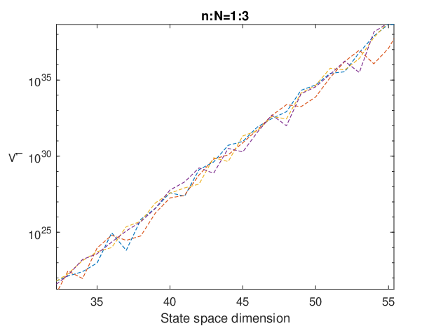

Statistics of largest singular value:
Preceding argument hints at strong spatial correalation, combined with results from the section on diagonalizable dynamics one can guess singular values are distributed non-uniformly also shown in (b) and (c) of figure 2: least singular value scales better than but largest singular value is that we aim to now formalize.
Theorem 4.1.
We can rigorously upper and lower bound norm of the iteration associated to action of matrix on invariant subspace , precisely given as:
| (26) |
where is the th power of the Jordan block corresponding to invariant subspace , with algebraic representation . corresponds to the row of the and represents the span of all the rows except the th one.
Proof.
First inequality follows from bounds on least singular value of , given in Lemma 1.3 of Chapter 1 in Vu 2014:
| (27) |
General upper bound follows by a simple variation of bounds provided in Tropp 2001 and last inequlaity under stability assumption is shown in Naeem 2023. ∎
Now w.l.o.g assume that for stable , i.e., that is only one eigenvalue with one eigenvector and generalized eigenvectors. Consequntly, and for grows as an exponential and then polynomially attaining a maxima and then starts decaying (see (d) of figure 2). Recall, conditioned on , we can express realization of the signal as: , along with preceding analysis explains blow up of largest singular value (see (c) of figure 2), which implies that distance between some or many of the row vectors and conjugate hyperplanes (defined as in 2.4) is becoming small.
5 Conclusion and future work:
In this paper we proposed a novel analysis for system identification, via running a single trajectory. Our analysis is based on concentration of measure phenomenon and tools developed in random matrix theory, making it naturally apt for high dimensional dynamical systems. Some of the important results and suggestions: qualitatively different behavior of diagonalizable and non-hermitian dynamical systems. Failure of OLS on non-hermitian systems, stems from the strong spatial correlations. Explosive diagonalizable dynamics, have large variance and distance between associated hyperplane and random vector can be small with high probability, thus deteriorating performance of OLS. Our analysis offers new and deep insights into learning for dynamical systems by studying the problem in Frobenius norm. However, more effort is required to bring our analysis on non-hermitian systems at the same theoretical footing as in diagonalizable case, which is currently a work in progress.
References
- Barvinok (2005) Alexander Barvinok. Math 710: Measure concentration. Lecture notes, 2005.
- Blower and Bolley (2005) Gordon Blower and François Bolley. Concentration inequalities on product spaces with applications to markov processes. arXiv preprint math/0505536, 2005.
- COOK (2017) NICK COOK. Selected topics from the geometric theory of random matrices. 2017.
- Faradonbeh et al. (2018) Mohamad Kazem Shirani Faradonbeh, Ambuj Tewari, and George Michailidis. Finite time identification in unstable linear systems. Automatica, 96:342–353, 2018.
- Kato (2013) Tosio Kato. Perturbation theory for linear operators, volume 132. Springer Science & Business Media, 2013.
- Naeem (2023) Muhammad Abdullah Naeem. Learning and concentration for high dimensional linear gaussians: an invariant subspace approach. arXiv preprint arXiv:2304.01708, 2023.
- Naeem and Pajic (2022) Muhammad Abdullah Naeem and Miroslav Pajic. Transportation-inequalities, lyapunov stability and sampling for dynamical systems on continuous state space. arXiv preprint arXiv:2205.12448, 2022.
- Oymak and Ozay (2021) Samet Oymak and Necmiye Ozay. Revisiting ho–kalman-based system identification: Robustness and finite-sample analysis. IEEE Transactions on Automatic Control, 67(4):1914–1928, 2021.
- Rudelson and Vershynin (2009) Mark Rudelson and Roman Vershynin. Smallest singular value of a random rectangular matrix. Communications on Pure and Applied Mathematics: A Journal Issued by the Courant Institute of Mathematical Sciences, 62(12):1707–1739, 2009.
- Sarkar and Rakhlin (2019) Tuhin Sarkar and Alexander Rakhlin. Near optimal finite time identification of arbitrary linear dynamical systems. In International Conference on Machine Learning, pages 5610–5618. PMLR, 2019.
- Sarkar et al. (2019) Tuhin Sarkar, Alexander Rakhlin, and Munther A Dahleh. Finite-time system identification for partially observed lti systems of unknown order. arXiv preprint arXiv:1902.01848, 2019.
- Simchowitz et al. (2018) Max Simchowitz, Horia Mania, Stephen Tu, Michael I Jordan, and Benjamin Recht. Learning without mixing: Towards a sharp analysis of linear system identification. In Conference On Learning Theory, pages 439–473, 2018.
- Tao (2012) Terence Tao. Topics in random matrix theory, volume 132. American Mathematical Soc., 2012.
- Tao et al. (2010) Terence Tao, Van Vu, and Manjunath Krishnapur. Random matrices: Universality of esds and the circular law. 2010.
- Tropp (2001) Joel A Tropp. An elementary proof of the spectral radius formula for matrices. 2001.
- Tsiamis and Pappas (2021) Anastasios Tsiamis and George J Pappas. Linear systems can be hard to learn. In 2021 60th IEEE Conference on Decision and Control (CDC), pages 2903–2910. IEEE, 2021.
- Tsiamis and Pappas (2022) Anastasios Tsiamis and George J Pappas. Online learning of the kalman filter with logarithmic regret. IEEE Transactions on Automatic Control, 2022.
- Vu (2014) Van H Vu. Modern aspects of random matrix theory, volume 72. American Mathematical Society, 2014.