Minimizing CNOT-count in quantum circuit of the extended Shor’s algorithm for ECDLP
Abstract
Since the elliptic curve discrete logarithms problem (ECDLP) was proposed, it has been widely used in cryptosystem because of its strong security. Although the proposal of the extended Shor’s algorithm offers hope for cracking ECDLP, it is debatable whether the algorithm can actually pose a threat in practice. From the perspective of the quantum circuit of the algorithm, we analyze the feasibility of cracking ECDLP with improved quantum circuits using an ion trap quantum computer.
We give precise quantum circuits for extended Shor’s algorithm to calculate discrete logarithms on elliptic curves over prime fields, including modulus subtraction, three different modulus multiplication, modulus inverse, and windowed arithmetic. Whereas previous studies mostly focused on minimizing the number of qubits or the depth of the circuit, we minimize the number of CNOTs, which greatly affects the time to run the algorithm on an ion trap quantum computer. First, we give the implementation of the basic arithmetic with the lowest known number of CNOTs and the construction of an improved modular inverse, point addition, and the windowing technique. Then, we precisely estimate the number of improved quantum circuits needed to perform the extended Shor’s algorithm for factoring an -bit integer, which is . We analyze the running time and feasibility of the extended Shor’s algorithm on an ion trap quantum computer according to the number of CNOTs. Finally, we discussed the lower bound of the number of CNOTs needed to implement the extended Shor’s algorithm.
Keywords:
Elliptic curve discrete logarithm problem , Extended Shor’s algorithm , Quantum circuits , Ion trap quantum computer ,Introduction
Elliptic curve cryptography (ECC) has attracted wide attention for its unique advantages since it was introduced in 1980s Miller 1985, Koblitz 1987.The safety of ECC is based on the elliptic curve discrete logarithm problem(ECDLP), which is the discrete logarithm problem (DLP) on the cyclic subgroup with a point on the elliptic curve as the generator and more complex than DLP. Although there are many attempts to solve DLP, the best known classical algorithm for DLP is still exponentially complex Miyaji 1992. Fortunately, with the development of quantum computing, the emergence of quantum algorithms offers hope for solving such problems. The most representative and compelling quantum algorithm is Shor’s algorithm Shor 1994, Shor 1999, which can theoretically solve DLP over multiplicative group for the prime fields in polynomial time Shor 1994, Shor 1999. This algorithm can be extended to elliptic curve groups (we call it extended Shor’s algorithm in this paper), which makes ECDLP theoretically not difficult to a quantum computer, thus posing a threat to the cryptography system based on ECDLP. However, the gates number of a quantum algorithm’s circuit determines the time to run the quantum algorithm on a quantum computer and the exact quantum gates number of the extended Shor’s algorithm has not been analyzed. Therefore, it is debatable whether the extended Shor’s algorithm can pose a threat to ECC, which is exactly what we are trying to do.
Quantum computers implement quantum computation by taking as input superposition quantum states representing all the different possible inputs and simultaneously evolving them into the corresponding outputs using a sequence of unitary transformations Yao 1993, Nielsen and Chuang 2002, Chiribella et al. 2008, Dong et al. 2013, Nash et al. 2020, Kimura et al. 2021, Liu et al. 2021, Liu et al. 2022, Gao et al. 2022. Quantum computing can be described as a quantum circuit in which the unitary transformations are represented by quantum gates. The most basic quantum gates are control-NOT (i.e., CNOT) and single qubit gates. In an ion trap quantum computer, the operation time of the non-adjacent CNOT is much higher than that of other single quantum gates, and the CNOT can only operate serially Yang and Zhou 2013. Therefore, the number of CNOT contained in the quantum circuit of a quantum algorithm largely determines the running time of the quantum algorithm.
Since the advent of the first quantum algorithm to attack ECC in 1995 Boneh and Lipton 1995, the research in this field has attracted extensive attention. Refs. Eicher and Opoku 1997, Proos and Zalka 2003, Kaye and Zalka 2004 proposed quantum algorithms that attack ECDLP defined on finite fields and , respectively. Ref.Roetteler et al. 2017 studied the extended Shor’s algorithm to attack ECDLP on and improved the algorithm of modular inversion in Proos and Zalka 2003. The resources needed from the Toffoli gates point of view were , but only rough results were given for the CNOT gates. Ref. Häner et al. 2020 improved the Kaliski algorithm in the middle of Roetteler et al. 2017. Fewer T gates were used in the circuit of modular inversion and the windowed arithmetic in Ref. Gidney 2019 was briefly introduced to calculate ECDLP, but it is not discussed in detail. In view of the size of the quantum computer, i.e. the number of qubits, a quantum circuit for calculating the discrete logarithm problem on a binary elliptic curve is optimized in Ref. Banegas et al. 2021.
Note that the resources required by the quantum circuit in previous papers did not analyse the number of CNOT gates in detail, but with the development of ion trap quantum computer, the number of CNOT gates largely determines the algorithm running time Knight et al. 1999. Therefore, this paper analyzes the feasibility of the quantum algorithm to attack ECDLP by studying the number of CNOT gates in the circuit and discusses the application of windowed arithmetic in detail. It is worth noting that based on the physical limitations of quantum computers, we consider whether a sufficiently large quantum computer in the future can complete the extended Shor’s algorithm in a reasonable running time, so we do not focus on the number of qubits.
Our contributions
In this paper, we give precise quantum circuits for the extended Shor’s algorithm to calculate discrete logarithms on elliptic curves over prime fields. More specifically, we have the following contributions.
- 1.
We construct and improve the circuits of basic operations including modulus subtraction, three different modulus multiplication, modulus inverse, windowed arithmetic and further improve the quantum circuit of extended Shor’s algorithm.
- 2.
We combine window technique to focus on optimizing the number of CNOT gates, and further analyze the running time of extended Shor’s algorithm on ion trap quantum computers according to the CNOT gates number we obtained.
- 3.
We study whether the extended Shor’s algorithm can be completed in a reasonable running time under the premise that the fault-tolerant quantum computer has enough space, further illustrating whether the Shor’s algorithm can really pose a threat to cryptosystems such as ECC.
Outline
The rest of the paper is organized as follows. Preliminaries section is the introduction of ECDLP and the elliptic curves group law. Quantum circuits for algebraic problems section introduces the basic circuits to compute scalar multiplication on the elliptic curves groups required by the algorithm, including modular multiplication, modular inverse, and windowed arithmetic, etc.. In Quantum circuits of point addition on elliptic curves groups section, we design a new method to calculate the point addition reversibly out-of-place (storing the results in a new register), which is different from the way of in-place (replacing the input value by the sum) in Roetteler et al. 2017 and reduces the CNOT number. The Discusion and conclusion section is a discussion of the time required to attack ECDLP.
Preliminaries
In this section, we first give a brief description of DLP, and then show the Shor’s algorithm for solving DLP. Next, we elaborate on the algorithm for solving ECDLP, which we call the extended Shor’s algorithm.
Shor’s quantum algorithm for solving the DLP
DLP. Let be a generator of a finite cyclic group with the known order , i.e . The DLP over is defined as, given an element , determining the unique such that , then . Consider the case when G is the additive group , where is a positive integer and . Here the DLP is to find satisfying . The DLP over the can be solved by finding the multiplicative inverse of modulo with the extended Euclidean algorithm in polynomial time Proos and Zalka 2003. However, in group (i.e., the multiplicative group modulo and ), there was no classical algorithm to solve the DLP (i.e., calculate ) until Shor Shor 1994, Shor 1999 in 1994 proposed a quantum algorithm that could theoretically solve this problem in polynomial time.
Shor’s quantum algorithm. To be specific, the Shor’s algorithm uses three quantum registers to solve the DLP, each quantum register has qubits and satisfies . The Shor’s algorithm for DLP is shown as follows.
| (1) |
| (2) |
| (3) |
| (4) |
Using the above algorithm, Shor proved that can be calculated with high probability in polynomial time. Based on the Shor’s algorithm to solve DLP, next we show the case of ECDLP.
Extended Shor’s quantum algorithm for solving the ECDLP
ECDLP. Let be a field of characteristic . An elliptic curve over is the set of solutions to the equation
| (5) |
where satisfy , together with the point at infinity. The set of all the points on the elliptic curve is . Then forms Abelian group with a point addition operation and as the neutral element. Let be a generator of , which is a cyclic subgroup of of known order , i.e., . Similar to DLP, the goal of ECDLP is to find the unique integer such that , where and is a given point in . Hasse Hasse 1936 pointed out that the number of all the points on the elliptic curve is . Thus the order of is no larger than . Therefore, when analyzing ECDLP on , the order can be set to , which has no effect on the results.
Extended Shor’s quantum algorithm. Different from the Shor’s quantum algorithm, the extended Shor’s algorithm uses two -qubit and one -qubit registers with to solve the ECDLP. The specific algorithm for ECDLP is shown as follows.
| (6) |
| (7) |
| (8) |
The initial state of the third register is instead of to satisfy the point addition rule on the elliptic curve. Whether we use or has no effect on the result of measuring probability. The detailed proof can be seen in the Appendix.
Elliptic curves group law
Before designing the circuits of the extended Shor’s quantum algorithm, The elliptic curve group law on an affine Weierstrass curve we give the law on the group of elliptic curves.
Let , the elliptic curve group law on the Eq. (5) can be computed as follows:
| (9) |
where satisfies the following equation:
| (10) |
Thus we have
| (11) |
Refs. Proos and Zalka 2003, Roetteler et al. 2017, Häner et al. 2020 described the detailed steps of how to transform coordinates from to . Since the purpose of this paper is to reduce the number of CNOT gates, we improve the previous steps of the coordinate transformation in Quantum circuits of point addition on elliptic curves groups to reduce the number of CNOT gates but at a cost of increasing the number of qubits, which is not the focus of this paper.
Quantum circuits for algebraic problems
In the implementation of the extended Shor’s algorithm for ECDLP, the most important is to design a quantum circuit to compute scalar multiplication on the elliptic curves groups, i.e., , which includes a series of modular operations. In this section, we design the circuits of modular subtraction and direct modular multiplication operations. Meanwhile, we improve a series of basic operations as well as including modular inversion and windowed arithmetic. In the following, the black triangle symbol in the circuits indicate that the corresponding qubit register is modified and holds the result of computation.
Modular subtraction
Modular subtraction is divided into four parts: controlled and non-controlled constant modular subtraction, controlled and non-controlled quantum state modular subtraction. The difference between the constant and the quantum state is that the constant is known and can be ignored in quantum circuits.
Modular subtraction of a constant , where is a known constant and is the known -bit constant, can be constructed by the following steps:
- 1.
Subtract from to using inverse circuit of the addition.
- 2.
If the highest bit of is corresponding to , then add to . Otherwise, do not operate.
- 3.
Compare the result of step with . Uncompute the auxiliary bit and get .
Next we give the detailed of the quantum circuit for performing addition and comparison.
(i) We use two circuits, and , to perform addition, i.e., . The first two quantum registers both have qubits and the third one has qubit as the highest bit of the sum. The two circuits of addition are shown below.
①: -
Ref. Cuccaro et al. 2004 presented a way to calculate the addition as shown in Fig. 1, which we denote by -. It shows that each (i.e., compute the majority of three bits in place) and each (i.e., UnMajority and Add) contain two CNOT gates and one Toffoli gate. Thus, -qubit has a total s and s, that is, CNOT gates and Toffoli gates. At the same time, based on the standard decomposition of the Toffoli gate into the Clifford+T set, we obtain that one Toffoli gate contains six CNOT gates Nielsen and Chuang 2002. Therefore, we conclude that the number of CNOT gates of an -qubit is . According to -, we further design its controlled form in Fig. 2 with a CNOT number of .


②: -
Vedral et al. Vedral et al. 1996 proposed another quantum circuit for calculating addition as shown in Fig. 3, where the blocks of and are shown in Fig. 4 and the circuit of is the inverse order of the quantum gates in . When the addend is known, Markov et al. Markov and Saeedi 2012 modified the to the form shown in the last two rows of Fig. 4, that is, the is omitted. At this point, one (or ) contains on average Toffoli gate and CNOT, and one has on average CNOT. Therefore, an -qubit - has a total s, s, and additional CNOT. Combine with six CNOT of one Toffoli, we conclude that the number of CNOT in is when y is known.


The left circuit in Fig.5 is a common controlled form of -, while the right one proposed by Ref. Häner et al. 2020 gives a simpler controlled form. That is, the control bits use NOT gates to control the known addend to store in an -qubit auxiliary register, then the addend cannot be omitted and need to use - to sum. Finally, repeat the storage operation to restore the auxiliary bits. Since encoding a known -qubit addend into the circuit requires an average of CNOTs, combined with the , we conclude that - requires CNOTs.


(ii) Now we also use two circuits, - and -, to perform comparison. Compare and by whether the highest bit of is or . When the highest bit is then , otherwise . The difference between these two circuits is that - applies to the case where is a known constant, while - can be used either for known or for unknown. Although we use - for all the comparisons covered in this paper, both circuits are presented for the sake of the completeness of the method. Details of the two circuits are shown below.
①: -
- in Fig. 6 is obtained by modifying - so that it output only the highest bit of Markov and Saeedi 2012. But the premise is that the input is instead of , which means this way only works if is a known constant instead of an unknown quantum state.

When is known, the can be simplified to Fig. 7, that is, one contains Toffoli. Thus the number of CNOT in is .

②: -
Although the 1- does not work when the minus is an unknown quantum state, it can be modified to not precompute . The specific steps are as follows. Firstly, input and flip each of the bits to get . Then use 1- to get the highest bit of , the flip of and . Finally, flip each of the bits and the highest bit of to recover and get which means the the highest bit of . Following above steps to obtain 2- as shown in Fig. 8. We see that - not only applies to where is a known constant but also applies to an unknown quantum state. The number of CNOT in the former is , which is the same as 1-, and the latter is . Fig. 9 is the controlled form of 2-. The corresponding CNOT numbers are and , respectively.


After showing the circuits of addition and comparison in steps (i) and (ii), we design the constant modular subtraction circuit in Fig. 10, which contains one , one CNOT, one , one with the known constant , and two circuits of encoding . Thus we conclude that the number of CNOT in is . Calculate using the reversible circuit of , which denotes .

The quantum state modular addition circuit can be obtained in a similar way, which is shown in Fig. 11. Different from the constant modular addition, contains one , two with the known constant , two CNOTs, one , and two circuits of encoding . Thus, we conclude that the number of CNOTs in is . Furthermore, using the reversible circuit we can calculate quantum state modular subtraction.

The controlled form of and are shown in Fig. 12 and Fig. 13, respectively. The corresponding CNOTs numbers are and , respectively.


Negation
Given the value of , it is easy to calculate algebraically. Conversely, performing this calculation using quantum circuit is difficult. In order to solve this problem, Markov et al. Markov and Saeedi 2012 indicated that it can be done by first flipping each of the bits to get , then subtracting from to get the result. According to these two steps, Fig. 14 shows the circuit of calculating and Fig. 15 is its controlled form. The number of CNOT is equal to in , i.e. , while in controlled circuit is .


Modular shift
For constructing the circuit of modular shift, i.e., , we first show the circuits of the binary shift. The functions of the binary shift are as follows.
| Left shift : | |||
| Right shift : |
Before the method to implement shift is to use SWAP gate, that is, the second method below. However, we note that there is no need to swap two qubits with a SWAP operation if a qubit is known to be in the state of . Hence, we reconstruct the modular shift circuit for an -qubit quantum register to reduce the CNOT number, that is, the first method below.
①The first shift method shown in Fig. 16 requires CNOT, and the controlled form uses one control qubit to control each CNOT, which needs Toffoli gates. Thus, the controlled form needs CNOT.

②The second shift method shown in Fig. 17 requires CNOT. Different from the first method, the controlled form of second method just needs to use one qubit to control the middle CNOT in each SWAP gate. Then the circuit requires CNOTs and Toffoli gates in total, that is, CNOT.


Based on the above two method to perform modular shift, we can choose an appropriate circuit to minimize the number of CNOT gates, that is, choose the second way when a controlled mode is involved, otherwise, choose the first method.
As shown in Figure 18, we improve the modular shift, by replacing the subtraction of the constant with a comparison of the constant . The CNOT count of our modular doubling is by selecting the appropriate binary shift method.

Modular multiplication
There are three kinds of modular multiplication methods: fast modular multiplication, Montgomery modular multiplication and direct modular multiplication. The first way is to compute by repeating modular and conditional modular additions. The second way is often the most efficient choice for modular multiplication when modulus is not close to a power of . The last method is to calculate it in the most direct way, that is, first do the binary multiplication and then subtract multiples of .
Fast modular multiplication. In Ref. Proos and Zalka 2003, the fast modular multiplication is used to calculate the modular multiplication and the circuit of this method is designed in detail in the section 3.3 of Ref. Roetteler et al. 2017, which requires CNOTs. Furthermore, module addition and module shift in the fast modular multiplication apply the circuits mentioned earlier in this paper.
Montgomery modular multiplication. According to the Montgomery algorithm Kaliski 1995, input , we can get , where and Roetteler et al. Roetteler et al. 2017 gave a specific quantum circuit. Combined with the basic arithmetic circuit improved before in this paper, appropriate circuits are selected to obtain the following Montgomery modular quantum circuit, the result in - is , where the is 1-, is the constant subtraction 2-. The inverse operation - is used to restore the auxiliary bits. The entire quantum circuit of Montgomery modular multiplication is a combination of - and - with a CNOT number of . Actually, to obtain the value , we still need to set CNOTs to encode the value into an extra -qubit auxiliary bits before performing -.

Direct modular multiplication. Now we give a method to construct the circuit of modular multiplication according to its calculation. The main idea is that , where , so , thus
Then by comparing the sizes of and to obtain the target result. Since this method is constructed directly according to the calculation, we call it direct modular multiplication. More specifically, it is divided into the following four steps.
- 1.
Calculate the value of .
- 2.
Calculate the value of , i.e., . If the highest bit of the result is 1, then add to the result.
- 3.
Repeat step until ;
- 4.
Repeat the reverse of steps in sequence to recover the auxiliary qubits.
According to the first three steps, we can obtain the following partial quantum circuit -. The circuit of step to restore the auxiliary bit is denotes -, i.e. the inverse operation of -, where the and are 1- and 2- respectively in Fig. 20. Thus the whole quantum circuit of direct modular multiplication needs CNOTs. Similar to the Montgomery modular multiplication, to obtain the value we still need to set CNOTs to encode the value into an extra -qubit auxiliary bits before performing -.

Modular inversion
The most common method of modular inverse is the extended Euclidean algorithm (EEA). Proos et al. Proos and Zalka 2003 described the idea of using EEA to calculate modular inverse and it required times of division in total and each step was performed times. However, implementing the EEA in a quantum circuit is very complicated, then we consider to use Montgomery inversion algorithm described in detail in Ref. Roetteler et al. 2017 and they repeated the Montgomery-Kaliski round function times to get . Subsequently, Haner et al. Häner et al. 2020 improved this algorithm and its circuit used fewer CNOTs, but used the same modular inversion circuit. In this paper, we choose the improved algorithm in Ref. Häner et al. 2020 as the round function and redesign a simpler circuit to calculate modular inversion.
For inputs , the Montgomery-Kaliski algorithm consists of two steps. First, calculate gcd and . Second, calculate . When the input quantum state is a superposition state, the number of iterations in the first step is related to the integer corresponding to a certain ground state. Considering all possible ground states in the superposition state, the first step requires rounds of iteration. However, before each round, it is necessary to judge whether the iteration process in the corresponding ground state has ended by determining whether is 0, so as to determine whether this round is really iterated. Due to , all ground states of the input superposition state need to go through the first rounds of iteration and only need to judge whether is 0 before the iteration of the last rounds. In the second step, the intermediate result is shifted to the right by bits. In the last -round iteration of the first step, the results of the subsequent ShiftMod of the second step is stored in the auxiliary qubit and is obtained.
Combining the round function circuit in Figure 6 (b) of Ref. Häner et al. 2020 with the above algorithm steps, the quantum circuit of the modular inversion in Fig. 21 is obtained. The quantum circuit for restoring the auxiliary bits is , i.e. the inverse operation of and the complete quantum circuit is a combination of and .

According to , we can obtain the whole quantum circuit of modular inversion needs CNOTs.
Windowed arithmetic
In this section, we use the window form described in Ref. Gidney 2019 to design the quantum circuit to attack ECDLP, reducing the CNOT number from to .
The general method to calculate by quantum circuit is to expand binary and control the operation of by using each bit of respectively, i.e.,
the circuit is shown in Fig. 22.

The circuit designed by this method is the point addition operation of -controlled. In Ref. Häner et al. 2020, it is pointed out that can be selected first and the cases represented by can be calculated and stored in an -qubit register, where .Then the is used to perform the point addition operation on the group of elliptic curves. The left circuit in Fig. 23 shows the situation when , where represents four cases of respectively. Only the abscissa of point is shown in the figure and CNOTs are required on average. Therefore, it is estimated that a total of Toffoli and CNOTs are needed for the calculation point , i.e., CNOTs.
In the case of , m-controlled CNOTs (i.e., Toffoli gates) and CNOTs are required in the circuit, so a total of CNOTs are required. However, we improve the circuit above to the right one in Fig. 23, thus we just need CNOTs when .


The Fig. 24 and Fig. 25 are the situation when and , respectively. According to the recursive formula, Toffoli and are required for with . Thus the total number of CNOT required can be reduced to .


Quantum circuits of point addition on elliptic curves groups
Before we describe the construction of basic arithmetic used in point addition on the elliptic curves groups. In this section, we design a new algorithm to calculate point addition reversibly out place (storing the results in a new register) which reduces the number of CNOT gate of modular inversion and modular multiplication compared to the in place(replacing the input value by the sum) given by Ref. Roetteler et al. 2017, while using qubits. Based on new approach for point addition, this section gives the schematic circuit of overall extended Shor’s algorithm for ECDLP and then applies windowed arithmetic Gidney 2019 to obtain the windowed scalar multiplication of the given point on elliptic curves.
Controlled form of point addition
Controlled form of point addition on elliptic curve, this algorithm operates on a quantum register holding the point , a control bit and ten auxiliary bits . The second point is assumed to be precomputed classical constant. If , the algorithm correctly calculates ; if .
| process | the change in value | |
| 1.1 | ||
| 2.1 | ||
| 3.1 | ||
| 4.1 | ||
| 5.1 | ||
| 6.1 | ||
| 7.1 | ||
| 8.1 | ||
| 9.1 | ||
| 10.1 | ||
| 11.1 | ||
| 12.1 | ||
| 13.1 |
| process | the change in value | |
| 13.2 | ||
| 12.2 | ||
| 11.2 | ||
| 10.2 | ||
| 9.2 | ||
| 8.2 | ||
| 7.2 | ||
| 6.2 | ||
| 5.2 | ||
| 4.2 | ||
| 3.2 | ||
| 2.2 | ||
| 1.2 |
Fig. 26 and Fig. 27 show quantum circuits corresponding to Table 1 and Table 2. The quantum registers all consist of logical qubits, whereas is a single logical qubits. Thus the number of CNOT is .

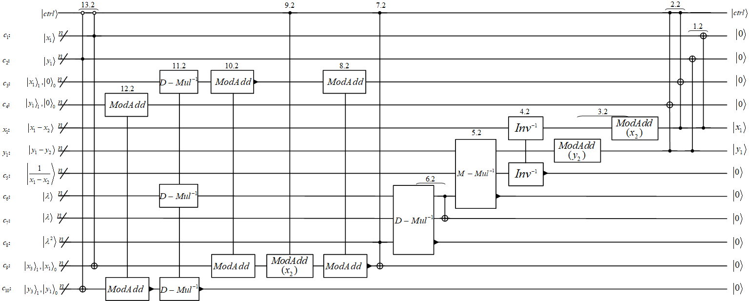
After each calculation of , the result will be used as the next input for a new calculation and then will be restored as an auxiliary bit. However, the result of the last calculation should be kept in the auxiliary register without any need to be restored. Therefore, the circuit of the last calculation is modified as shown in Fig. 28. And the number of CNOT is .

Therefore, the schematic quantum circuit of overall extended Shor’s algorithm for ECDLP can be obtained by combining the Fig. 26 to Fig. 28.

Windowed form of point addition
Windowed form of point addition on elliptic curve, this algorithm operates on a quantum register holding the point , and eight auxiliary bits. In this form, the second point is stored in the quantum register as a quantum state and cannot be precomputed as a classical constant.
Table 3 and Table 4 describe the process of calculating by windowed arithmetic and restoring auxiliary bits, respectively.
| process | the change in value | |
| 1.1 | ||
| 2.1 | ||
| 3.1 | ||
| 4.1 | ||
| 5.1 | ||
| 6.1 | ||
| 7.1 | ||
| 8.1 | ||
| 9.1 | ||
| 10.1 | ||
| 11.1 |
| process | the change in value | |
| 11.2 | ||
| 10.2 | ||
| 9.2 | ||
| 8.2 | ||
| 7.2 | ||
| 6.2 | ||
| 5.2 | ||
| 4.2 | ||
| 3.2 | ||
| 2.2 | ||
| 1.2 |
Fig. 30 and Fig. 31 show quantum circuits corresponding to Table 3 and Table 4. The quantum registers all consist of logical qubits. Thus the number of CNOT is .


After each calculation of , the result will be used as the next input for a new calculation and then will be restored as an auxiliary bit. However, the result of the last calculation should be kept in the auxiliary register without any need to be restored and the coefficients of and are different in the extended Shor’s quantum algorithm, it cannot be mixed in the application of using window arithmetic. Therefore, the circuit of the last calculation is modified as shown in Fig. 32 with .

Fig. 33 is the schematic quantum circuit to calculate ECDLP by the extended Shor’s algorithm using windowed arithmetic, where the is situation where several controlled operations can be merged into a single operation acting on a value produced by a small QROM lookup Gidney 2019 and the point addition is the circuit introduced in Fig. 30 to Fig. 33.

According to the process of calculating point addition, the number of CNOT gates for the first point addition is (including the circuits for recovering auxiliary bits) and the -th has CNOTs. Therefore, the number of CNOT needed to calculate the point addition of ECDLP using controlled point addition is . When using the form of window, modular subtraction of a constant is changed to and the CNOT number increases from to . At the same time, the number of CNOT in the controlled circuit increases from to , thus the number of CNOT gates for the first point addition is and the -th has CNOTs in calculating . so the number of CNOT needed to calculate the point addition of ECDLP using the form of Window is .
Now we analyze the whole circuit of the extended Shor’s algorithm to obtain a specific CNOT number. It can be inferred from the form of the formula that only when , is a polynomial function of . We calculate , and for each , we use Matlab to approximate the zero of to obtain a pair . Because should be an integer, we round each up and down to get and , respectively. Then letting for each and fitting with respect to based on all the pairs , we obtain . Combine the CNOT gates used for two , then there has the total number of CNOT of the extended Shor’s algorithm for ECDLP is . Ref. Yang and Zhou 2013 gives the lower limit of time for executing a CNOT gate in an ion trap quantum computer, which is about . Combined with the number of CNOT to run the extend Shor’s algorithm, the time to break -bit ECDLP takes at least years after three levels of coding.
Discusion and conclusion
Although there have been many attempts to improve the qubit number or the circuit depth of the extended Shor’s algorithm for ECDLP, their focus has not been on optimizing the number of CNOT gates, which greatly affects the time to run the algorithm in an ion trap quantum computer. In this paper, we improve the quantum circuit of basic arithmetic operations, including modulus subtraction, three different modulus multiplication, modulus inverse and windowed arithmetic. Table 5 summarizes the CNOT numbers for the basic arithmetic. We further improve the quantum citcuit of extended Shor’s algorithm. Based on this work, the quantum circuit that run the extended Shor’s algorithm is greatly improved. We reduce the CNOT gates number from to , and calculate the specific number of CNOT gates required by the algorithm. The time required by the extended Shor’s algorithm to attack -bit ECDLP are estimated, i.e., years, which means it is hard to attack ECDLP using ion trap quantum computer in a reasonable time. However, this estimated time does not take into account the fault tolerance of the circuit, which we will study in the future.
According to the results of CNOT number, we can consider the lower bound of CNOT number required by the extended Shor’s algorithm. If we assume that the time required to run extended Shor’s algorithm is , the time required to execute a CNOT is , and the lower bound of the number of CNOTs is , which is a function of the number of qubits . Thus, the lower bound of the run time of the extended Shor’s algorithm can be expressed as . Modular inverse can be constructed using the basic arithmetic operations, such as modular addition. Therefore, the number of CNOTs required for modular inverse must be greater than that required for modular addition. Because the quantum circuit of modular addition adds a modular operation, the number of CNOTs required by modular addition must be larger than that of the addition circuit. For two qubits , we have that , where and are the - bits of the binary representation of , is the - carry, and is the sum of the - bits. Therefore, each qubit addition requires at least one Toffoli and three CNOTs. Thus, the addition of qubits requires at least CNOTs. However, we have not obtain a specific lower bound of the number of CNOT gates required to run the extended Shor’s algorithm, so we plan to calculate the lower bound more tight in our next work.
| The basic arithmetic | Number of Toffoli | Number of CNOT | Total number of CNOT |
| 1-Addy (unknown ) | |||
| ctrl-1-Addy (unknown ) | |||
| 2-Addy (know ) | |||
| ctrl-2-Addy | |||
| 1-comp | |||
| 2-compy (know ) | |||
| ctrl-2-compy (know ) | |||
| 2-compy (unknown ) | |||
| ctrl-2-compy (unknown ) | |||
| Mod-Suby or Mod-Addy (know ) | |||
| ctrl-Mod-Suby (known ) | |||
| Mod-Addy (unknown ) | |||
| ctrl-Mod-Addy (unknown ) | |||
| neg | |||
| ctrl-neg | |||
| 1-shift | - | ||
| ctrl-1-shift | - | ||
| 2-shift | - | ||
| ctrl-2-shift | |||
| Shift-Mod | |||
| M-MM (half) | |||
| D-Mul (half) |
References
- Miller [1985] V. S. Miller, in Conference on the theory and application of cryptographic techniques (Springer, 1985) pp. 417–426.
- Koblitz [1987] N. Koblitz, Mathematics of computation 48, 203 (1987).
- Miyaji [1992] A. Miyaji, in International Workshop on the Theory and Application of Cryptographic Techniques (Springer, 1992) pp. 477–491.
- Shor [1994] P. W. Shor, in Proceedings 35th annual symposium on foundations of computer science (Ieee, 1994) pp. 124–134.
- Shor [1999] P. W. Shor, SIAM review 41, 303 (1999).
- Yao [1993] A. C.-C. Yao, in Proceedings of 1993 IEEE 34th Annual Foundations of Computer Science (IEEE, 1993) pp. 352–361.
- Nielsen and Chuang [2002] M. A. Nielsen and I. Chuang, “Quantum computation and quantum information,” (2002).
- Chiribella et al. [2008] G. Chiribella, G. M. D’Ariano, and P. Perinotti, Physical review letters 101, 060401 (2008).
- Dong et al. [2013] D. Dong, C. Chen, M. Jiang, and L.-C. Wang, “Quantum control and quantum information technology,” (2013).
- Nash et al. [2020] B. Nash, V. Gheorghiu, and M. Mosca, Quantum Science and Technology 5, 025010 (2020).
- Kimura et al. [2021] T. Kimura, K. Shiba, C.-C. Chen, M. Sogabe, K. Sakamoto, and T. Sogabe, Mathematical Problems in Engineering 2021, 1 (2021).
- Liu et al. [2021] X. Liu, H. Yang, and L. Yang, arXiv preprint arXiv:2112.11358 (2021).
- Liu et al. [2022] X. Liu, G. Liu, J. Huang, and X. Wang, arXiv preprint arXiv:2205.13539 (2022).
- Gao et al. [2022] W. Gao, L. Yang, D. Zhang, and X. Liu, Cryptography 6, 9 (2022).
- Yang and Zhou [2013] L. Yang and R.-R. Zhou, arXiv preprint arXiv:1305.5640 (2013).
- Boneh and Lipton [1995] D. Boneh and R. J. Lipton, in Annual International Cryptology Conference (Springer, 1995) pp. 424–437.
- Eicher and Opoku [1997] J. Eicher and Y. Opoku, (1997).
- Proos and Zalka [2003] J. Proos and C. Zalka, arXiv preprint quant-ph/0301141 (2003).
- Kaye and Zalka [2004] P. Kaye and C. Zalka, arXiv preprint quant-ph/0407095 (2004).
- Roetteler et al. [2017] M. Roetteler, M. Naehrig, K. M. Svore, and K. Lauter, in International Conference on the Theory and Application of Cryptology and Information Security (Springer, 2017) pp. 241–270.
- Häner et al. [2020] T. Häner, S. Jaques, M. Naehrig, M. Roetteler, and M. Soeken, in International Conference on Post-Quantum Cryptography (Springer, 2020) pp. 425–444.
- Gidney [2019] C. Gidney, arXiv preprint arXiv:1905.07682 (2019).
- Banegas et al. [2021] G. Banegas, D. J. Bernstein, I. van Hoof, and T. Lange, IACR Transactions on Cryptographic Hardware and Embedded Systems , 451 (2021).
- Knight et al. [1999] P. Knight, M. Murao, M. Plenio, and V. Vedral, (1999).
- Hasse [1936] H. Hasse, (1936).
- Cuccaro et al. [2004] S. A. Cuccaro, T. G. Draper, S. A. Kutin, and D. P. Moulton, arXiv preprint quant-ph/0410184 (2004).
- Vedral et al. [1996] V. Vedral, A. Barenco, and A. Ekert, Physical Review A 54, 147 (1996).
- Markov and Saeedi [2012] I. L. Markov and M. Saeedi, arXiv preprint arXiv:1202.6614 (2012).
- Kaliski [1995] B. S. Kaliski, IEEE transactions on computers 44, 1064 (1995).
Appendix
We first prove in detail that whether the input state of the third quantum register is or has no effect on the measurement probability. Then, we give the specific derivation process of the number of CNOT gates in the n-controlled-NOT.
The value of the input state has no effect on the result
Proof.
When the input state is , we have
where , so , thus the probability of getting a is
so when taking all of , the probability of is
| (12) |
When the input state is , we have
where , so , thus the probability of getting a is
so when taking all of , the probability of is
| (13) |
To prove that it doesn’t matter whether the input is or , just prove that
There has
Because , so we have , then . ∎
The number of CNOT gates in n-controlled-NOT
The Fig. 34 is the quantum circuit of n-controlled-NOT,

which can be contrusted by auxiliary qubits and Toffoli. The quantum circuit is as follows.
