Design of the Impulsive Goodwin’s Oscillator: A Case Study†
Abstract
The impulsive Goodwin’s oscillator (IGO) is a hybrid model composed of a third-order continuous linear part and a pulse-modulated feedback. This paper introduces a design problem of the IGO to admit a desired periodic solution. The dynamics of the continuous states represent the plant to be controlled, whereas the parameters of the impulsive feedback constitute design degrees of freedom. The design objective is to select the free parameters so that the IGO exhibits a stable 1-cycle with desired characteristics. The impulse-to-impulse map of the oscillator is demonstrated to always possess a positive fixed point that corresponds to the desired periodic solution; the closed-form expressions to evaluate this fixed point are provided. Necessary and sufficient conditions for orbital stability of the 1-cycle are presented in terms of the oscillator parameters and exhibit similarity to the problem of static output control. An IGO design procedure is proposed and validated by simulation. The nonlinear dynamics of the designed IGO are reviewed by means of bifurcation analysis. Applications of the design procedure to dosing problems in chemical industry and biomedicine are envisioned.
I INTRODUCTION
In control of engineered systems, the objective is normally to keep the controlled variable in a vicinity of a predefined setpoint or to make it follow a certain trajectory. In contast, the purpose of physiological control is, arguably, to maintain the involved biological quantities within a certain domain, and to achieve this with minimal energy. Impulsive feedback control is one of the most widespread strategies applied by nature in physiological, especially in neuroendocrine, systems. In particular, the hypothalamic-pituitary adrenal and gonadal axes employ pulse-modulated control and encode information to target cells by manipulating both the amplitude and frequency of the hormone concentration pulses [2].
The problem of exerting a periodic control action that maintains a certain predefined level of effect in a dynamical plant often arises in process control and medicine. For instance, adding doses of chemicals to a reactor is typically done by means of logical (discrete) open-loop control [3]. Similarly, pharmaceuticals, in a tablet or an injection form, are predominantly administered according to a regimen that is prescribed by a physician. When the plant is dissipative and no feedback is involved, the resulting control system is simple and safe. However, the open-loop control cannot attenuate disturbances and handle plant uncertainty.
Provided the actuators can be continuously manipulated and real-time measurements of the controlled variable are available, feedback control is routinely employed to achieve robust closed-loop stability or performance. When the control signal is however restricted to impulsive action, the only currently available feedback strategy is Model Predictive Control (MPC) [4]. The utility and physiological coherence of impulsive MPC in drug delivery applications is readily recognized. A promising application of this control approach to insulin dosing in simulated diabetes patients is reported in e.g. [5]. In fact, impulsive insulin delivery mimics the physiological profile of secreting around ten major hormone pulses over 24 hours [6] with their temporal distribution related to meals. Impulsive feedback control is inherently nonlinear and adding an advanced control law to the closed-loop dynamics further complicates stability and performance analysis. Yet, simple pulse-modulated feedback solutions manipulating the amplitude and frequency of the control impulses are lacking at present.
The Impulsive Goodwin’s Oscillator (IGO) was proposed [7, 8] as a hybrid (continuous-discrete) model of testosterone regulation in males, generalizing the concept of the original (continuous) Goodwin’s oscillator [9] to the case of pulsatile (non-basal) secretion. The IGO possesses a number of properties that are typically sought for in biomedical applications, e.g. positivity and boundedness of the solutions. By design, the IGO has no equilibria and can only exhibit periodic or non-periodic (chaotic and quasiperiodic) oscillations [10]. It is proven that the IGO always possesses a unique (stable or unstable) -cycle, i.e. a periodic solution with only one firing of the pulse-modulated feedback on the least period [8]. Extensive bifurcation analysis of the IGO [10] suggests that the model, being equipped with the modulation functions of Hill’s type, is monostable, even under a small delay present in the closed loop [11]. Thus, when in a stable periodic solution, the IGO is not likely to change to another type of solution due to a temporary exogenous disturbance.
This paper addresses a novel problem of designing an IGO that exhibits a stable 1-cycle with desired characteristics. The main contributions of the paper are threefold:
- •
the IGO design problem is formulated with respect to a desired solution, i.e. a 1-cycle;
- •
necessary and sufficient orbital stability conditions of the 1-cycle in the IGO are provided;
- •
bifurcation analysis of the nonlinear IGO dynamics in vicinity of the designed 1-cycle is performed.
The paper is organized as follows. In Section II, known facts about the dynamics of the IGO are summarized to facilitate further reading. In Section III, the problem of designing an IGO that exhibits a stable predefined 1-cycle is formulated and solved. A numerical example is considered in Section IV to illustrate the proposed design concept. Section V provides bifurcation analysis of the designed IGO to discern nonlinear dynamics phenomena arising under deviations of the nominal parameter values. Finally, conclusions are drawn.
II BACKGROUND
This section summarizes the facts pertaining to the IGO model and its behaviors that are used in the rest of the paper.
II-A The Impulsive Goodwin’s Oscillator
The IGO is given by the following equations [7, 8]
| (1) |
| (2) | ||||
where are constant matrices, ,
is the controlled output, and the state describes concentrations of some chemical substances. In continuous model part (1), are distinct constants and are positive gains. It is readily observed that the matrix is Hurwitz stable, also,
| (3) |
The latter property implies, in particular, that is a smooth function despite the jumps in (2).
The minus and plus in a superscript in (2) denote the left-sided and a right-sided limit, respectively. The amplitude modulation function and frequency modulation function are continuous and monotonic for positive arguments; is non-increasing and is non-decreasing, also,
| (4) |
where , , , are positive constants11 1 Notably, with respect to dosing applications, the bounds and specify the least and largest dose that can be delivered by the control law, while and prescribe the shortest and longest interval between the administered doses. The explicit way of enforcing these safety limits is favorable in, e.g., healthcare applications.. Then control law (2) constitutes a frequency and amplitude pulse modulation operator [12] implementing an output feedback over (1). The time instants are called (impulse) firing times and represent the corresponding impulse weights.
II-B Solution Properties
The dynamics of the IGO are defined by differential equation (1) in between the feedback firing times and undergo jumps of the magnitude at the times in accordance with (2). Due to the positivity of , the IGO lacks equilibria and exhibits only oscillatory periodic or non-periodic (e.g. chaotic or quasiperiodic) solutions. The solutions of the IGO are positive under a positive initial condition , because is Metzler22 2 A square matrix whose off-diagonal entries are all nonnegative is said to be Metzler. The exponential is nonnegative for a Metzler . and is uniformly positive due to (4). It is proved in [8] that the solutions are bounded, because is Hurwitz and the nonlinear characteristics are bounded.
Denoting , the evolution of the continuous state vector of the IGO from one firing time to the next one obeys the impulse-to-impulse map [8]
| (5) | ||||
This paper focuses on periodic solutions of model (1),(2) that correspond to fixed points of the map . A periodic solution with exactly firings of the pulse-modulated feedback within the least period is called -cycle. In particular, for a 1-cycle with the initial condition , it applies
| (6) |
Since all the solutions of (1), (2) are positive, it holds that , where the inequality is understood element-wise.
Proposition 1 ([8])
System (1), (2) has one and only one (positive) -cycle, that is, (6) has a unique solution . The cycle parameters , , and can be evaluated by solving the following system of algebraic equations
| (7) | ||||
| (8) |
The key idea of proving Theorem 1 in [8] is to rewrite (6) in terms of the output variable as
| (9) |
which equation is subsequently reduced to the scalar equation
The right-hand side of this equation is a decreasing bounded function of , being strictly positive as [8], which entails the existence and uniqueness of the solution.
The 1-cycle above is orbitally asymptotically stable [8] if and only if the fixed point is asymptotically stable as the equilibrium of discrete-time dynamics (5), that is, the Jacobian matrix is Schur stable33 3 A square matrix is said to be Schur (Schur stable) if all its eigenvalues belong to the unit disk ., where
| (10) |
III DESIGN
The IGO design problem treated here is formulated in the following way. Suppose that the dynamics of (1) given by the matrix are known. In drug dosing, the elements of can belong to, e.g., a known pharmacokinetic-pharmacodynamic model [13]. Given the parameters of a 1-cycle, the IGO design task is to find the modulation functions that render, with orbital stability, the desired periodic solution.
In terms of the model parameters, the problem in question can be summarized as follows. Given the parameters , find that provide the desired characteristics of a stable 1-cycle . In the design procedure proposed below, always appears in product with and can be selected as an arbitrary constant.
From (8) and (10), the conditions for 1-cycle existence and stability in the IGO involve , i.e. the output value at the fixed point in (6). Therefore, the modulation functions, as such, cannot be obtained in the design procedure, but only interpolation conditions that they and their derivatives have to satisfy to achieve the desired solution.
III-A Divided differences and the Opitz formula
To evaluate of a function of the matrix , the so-called Opitz formula will be used in the analysis to follow. The complex-valued function is assumed to be well-defined and complex-analytic in a vicinity of the matrix spectrum where the eigenvalues are pairwise different; See [14] for a more general case.
The first divided difference (1-DD) of a function is introduced [15, 16] as a function of two variables
which expression is well defined if and only if , exist and . The second divided difference (2-DD) is a function of three variables and is defined by
where exist and are pairwise different. Remarkably, both 1-DD and 2-DD are symmetric functions. Furthermore, for a scalar and , it holds
After some computations, it can be shown that
The Lagrange mean value theorem implies that if attains real values on some real interval , then, for each , there exists such that A similar result can be proved for the 2-DD [16, Corollary to Proposition 43]: for each triple , one has
For matrices of dimension three, a generalized44 4 Typically, the Opitz formula is considered for the situation where the second main diagonal contains ones, that is, , the general case can be derived by a simple similarity transformation. Opitz formula in [14] gives the closed-form representation of
For instance, one may compute explicitly the evolutionary matrix of the linear system (1) by applying the Opitz formula to function , where is constant:
Here, following standard notation, we use to denote the 1-DD of the exponential function ; the same applies to the 2-DD .
By virtue of the mean value theorem, all divided differences of the exponential function are positive. Subsequently, all the elements of are non-negative. This is well in line with the fact of being Metzler. The obtained expression for the transition matrix generalizes to higher dimensions of the continuous dynamics when the two-diagonal structure of the matrix is preserved [14].
III-B Fixed point
Proposition 1, combined with the Opitz formula, enables the calculation of the parameters of the unique 1-cycle for a given model of the IGO. The 1-cycle corresponds to a fixed point of the map , according to (6). The following converse statement, yielding the fixed point for a set of 1-cycle parameters, can then be proven.
Denote, for brevity,
Proposition 2
Given the parameters of -cycle , , the fixed point of map from (5) is calculated as
| (11) | ||||
| (12) | ||||
Proof:
For and , is a given fixed point satisfying (9) if and only if
that is, is the first column of the matrix . The leftmost equalities in (2), relating to the divided differences of , follow immediately from the Opitz formula. The rightmost equalities are validated by a straightforward computation, which is omitted here. ∎
Proposition 2 implies that can be calculated for any choice of the distinct constants , which fact perfectly agrees with the result of Proposition 1. Then, for a given continuous part of the IGO in (1) and desired , the value of is obtained by specifying the values of the modulation functions at that point according to (8). Further, since a 1-cycle is uniquely defined by the fixed point, the elements of the matrix and stipulate the periodic solution of the IGO.
III-C Stability of -cycle
Proposition 2 specifies the fixed point corresponding to the desired periodic solution but does not guarantee its stability. Then, additionally, matrix (10) needs to be stable to ensure that the 1-cycle is relevant in feedback control context.
In the design problem at hand, the slopes of the modulation functions , at the fixed point corresponding to the desired 1-cycle constitute the degrees of freedom that can be utilized for the stabilization of the periodic solution. As the result below explicates, the design problem is similar to what is known as static output feedback stabilization in linear time-invariant (LTI) systems [17].
Proposition 3
Proof:
The expression for and formulas for are straightforward from (10). Furthermore, since and all divided differences of the exponential functions are positive, the formula for derived in Section III-A ensures that the vector , being the first column of the matrix , is strictly positive. In order to prove that , notice that
Introducing the function
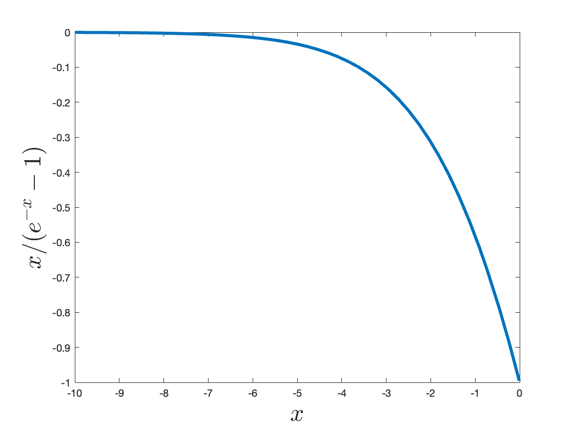
one notices that is nothing else but the first column of the matrix . It can be demonstrated that the function (see Fig. 1) is negative, decreasing, and strictly concave on the interval . Hence, in view of the mean value theorem, the divided differences , , are all negative, as well the values . In virtue of the Opitz formula, , entailing that and concluding the proof of Proposition 3. ∎
From the result of Proposition 3, can be rendered Schur stable by the feedback gain
| (13) |
subject to
| (14) |
Since the pair is observable, an arbitrary eigenvalue spectrum of can be achieved with an unrestricted gain . However, due to (14), has to be a linear combination of and with the coefficients and , correspondingly. This feedback structure also appears in the classical problem of static output feedback design, see [17] for an overview. A crucial distinction between the static output feedback in an LTI system and the pulse-modulated feedback of the IGO is that the former operates around a (constant) output setpoint whereas the latter stabilizes an LTI along a periodic solution (a 1-cycle) expressed as a fixed point.
Remark 1
The last statement of Proposition 3 entails that , for all feasible values of . Therefore, the feedback in the IGO is negative, despite the fact that all the involved quantities are positive. This property is natural given the underlying principle of the pulse-modulated feedback in the IGO where the impulses become of lower weight and sparser when the output values are higher than .
It can also be noticed that the pair of slopes yields in the Schur stable matrix . Even though constant modulation functions formally produce a stable 1-cycle, the feedback in the IGO is essentially eliminated, and the impulsive sequence is independent of the measured output.
Lemma 1 (Theorem 3.1, [18])
Let be a real matrix. Denote , where stand for the principle minors
Then, matrix is Schur stable if and only if the following three conditions are satisfied:
- 1.
,
- 2.
,
- 3.
.
To analyse the Schur stability of matrix (10), one can find the characteristics employed by Lemma 1 as functions of , . For instance, applying (13) and the well-known Schur complement formula , where are square matrices, but need not be square, one has
To derive the latter equality, one has to notice that . Similarly, after some computations, one can obtain two remaining characteristics. We formulate the following proposition.
Proposition 4
III-D Design algorithm
The results of Section III can be summarized in the form of the following procedure rendering the desired solution to the IGO.
- Step 1:
Select the desired 1-cycle’s characteristics and .
- Step 2:
From plant model (1), obtain the parameters , , and ; can be selected arbitrarily.
- Step 3:
Calculate the fixed point (and ) from (2).
- Step 4:
Define the structure of the modulation functions , and calculate their derivatives , .
- Step 5:
- Step 6:
By selecting the parameters of the modulation functions, ensure that , satisfy the stability conditions of Step 5.
- Step 7:
By scaling the modulation functions, ensure the equalities , .
IV DESIGN EXAMPLE
This section illustrates the use of the design algorithm outlined in Section III-D by a numerical example worked out step-by-step.
Consider the design of a 1-cycle with , (Step 1) in the IGO given by (1), (2), where , , , , , and , (Step 2). The corresponding fixed point (Step 3)
thus . Following [8], define the structure of the modulation functions (Step 4) as the Hill functions
| (15) | |||
The coefficients explicitly specify the values on the minimal and maximal dose as well as the minimal and maximal time interval between the doses
The parameters and also influence the derivatives of the modulation functions
Therefore, besides , , the derivatives are also defined by , , , .
From the parameters of continuous part (1) and , the stability conditions of the fixed point are evaluated. Then the involved functions of the Jacobian amount to
Notice that for all admissible values of , . Given the orders of the coefficients in the matrix functions of , stability of is guaranteed if
or, due to the positivity of ,
| (16) |
The inequality above is satisfied for , . As expected, stability condition (16) limits the derivatives of the modulation functions that act as feedback gains, cf. (14). Also , have to obey certain inequalities imposed by the parametrization in (15).
Introduce the notation
Then, for to take the desired value in , it applies
and, therefore,
When it is guaranteed that
| (17) |
both and are positive, then
Similarly, with
one has
and then
When it is guaranteed that
| (18) |
both roots are positive. Notice that the condition
results in a weaker inequality
Conditions (17) and (18) are satisfied (Step 5) for , thus yielding , , . Now, and ensures (Step 6) that
The closed orbit of the designed 1-cycle is depicted in Fig. 2, along with trajectories resulting from deviations in initial conditions for continuous part of the IGO (1). The evolution of the impulse weight (dose) sequence (see (2)) to the pre-defined 1-cycle amplitude is depicted in Fig. 3. A series of interchanging overdosing and underdosing events asymptotically converges to the desired value. This behavior could not be predicted from the design procedure since only a stable 1-cycle is sought.


V BIFURCATION ANALYSIS
To investigate the behaviors of the designed IGO under parameter variation, bifurcation analysis is performed. For an interval of the parameter values and following the steps of the design procedure in Section III, the value of is found and the stability of a fixed point is evaluated. The condition is imposed to reduce the number of independent bifurcation parameters.
From Section III-D, ; ; ; ; ; . For each , the value of is found by solving equations (15) with , and the stability of a fixed point of mapping (5) given by Proposition 2 is analyzed.


An example of such an analysis is shown in Fig. 4 (a),(b) for , , and . When the parameter increases, the fixed point undergoes a period-doubling bifurcation: the maximal in absolute value multiplier of the fixed point emerges from the unit circle though (see Fig. 4(b)). In these figures, the stability region of the fixed point is in yellow. Fig. 4(b) depicts the dependence of on in the transition shown in Fig. 4(a).
Fig. 4(c),(d) presents the results of the bifurcation analysis for other values of the cycle parameters: , and . As pointed out earlier, the stability of the fixed point (1-cycle) is determined by and .
Introduce as
The value of characterizes the convergence time of the trajectory initiated a point in the basin of attraction of the stable fixed point to the corresponding orbit.
Fig. 5(a),(b) show variation of the and in the intervals and for and (, ), respectively.


VI CONCLUSIONS
A novel problem of designing the IGO to admit a pre-defined periodic solution is introduced. It is exemplified by a case of stable 1-cycle with pre-defined solution parameters. It is demonstrated that the 1-cycle specifications are translated into a unique positive fixed point of the impulse-to-impulse discrete map. This fixed point can be rendered stable by selecting the modulation functions of the IGO. Further analysis is needed to control the type (monotonous, non-monotonous) and the speed of convergence of the IGO solutions to the orbit corresponding to the obtained fixed point.
References
- [1] A. Medvedev, A. Proskurnikov, and Z. T. Zhusubaliyev, “Design of the impulsive goodwin’s oscillator: A case study,” in American Control Conference, 2023.
- [2] J. Walker, J. R. Terry, K. Tsaneva-Atanasova, S. Armstrong, C. McArdle, and S. L. Lightman, “Encoding and decoding mechanisms of pulsatile hormone secretion,” J Neuroendocrinol., vol. 22, no. 12, pp. 1226–1238, December 2010.
- [3] J. Alford and G. Hida, “Discrete systems in process control,” AIChE CEP magazine, pp. 57–63, June 2022.
- [4] P. Sopasakis, P. Patrinos, H. Sarimveis, and A. Bemporad, “Model predictive control for linear impulsive systems,” IEEE Transactions on Automatic Control, vol. 60, no. 8, pp. 2277–2282, 2015.
- [5] P. S. Rivadeneira, J. Godoy, J. Sereno, P. Abuin, A. Ferramosca, and A. González, “Impulsive MPC schemes for biomedical processes: Application to type 1 diabetes,” in Control Applications for Biomedical Engineering Systems, A. T. Azar, Ed. Academic Press, 2020, pp. 55–87.
- [6] K. Polonsky, B. D. Given, and E. Van Cauter, “Twenty-four-hour profiles and pulsatile patterns of insulin secretion in normal and obese subjects,” J Clin Invest., vol. 81, pp. 442–448, February 1988.
- [7] A. Medvedev, A. Churilov, and A. Shepeljavyi, “Mathematical models of testosterone regulation,” in Stochastic optimization in informatics. Saint Petersburg State University, 2006, no. 2, pp. 147–158, in Russian.
- [8] A. Churilov, A. Medvedev, and A. Shepeljavyi, “Mathematical model of non-basal testosterone regulation in the male by pulse modulated feedback,” Automatica, vol. 45, no. 1, pp. 78–85, 2009.
- [9] B. C. Goodwin, “Oscillatory behavior in enzymatic control processes,” in Advances of Enzime Regulation, G. Weber, Ed. Oxford: Pergamon, 1965, vol. 3, pp. 425–438.
- [10] Z. T. Zhusubaliyev, A. Churilov, and A. Medvedev, “Bifurcation phenomena in an impulsive model of non-basal testosterone regulation,” Chaos, vol. 22, no. 1, pp. 013 121–1—013 121–11, 2012.
- [11] A. Churilov, A. Medvedev, and Z. T. Zhusubaliyev, “Impulsive goodwin oscillator with large delay: Periodic oscillations, bistability, and attractors,” Nonlinear Analysis: Hybrid Systems, vol. 21, pp. 171–183, 2016.
- [12] A. K. Gelig and A. N. Churilov, Stability and Oscillations of Nonlinear Pulse-modulated Systems. Boston: Birkhäuser, 1998.
- [13] H. Runvik, A. Medvedev, and M. C. Kjellsson, “Impulsive feedback modeling of levodopa pharmacokinetics subject to intermittently interrupted gastric emptying,” in 2020 American Control Conference (ACC), 2020, pp. 1323–1328.
- [14] A. V. Proskurnikov, H. Runvik, and A. Medvedev, “Cycles in impulsive goodwin’s oscillators of arbitrary order,” 2023, under review, available as arXiv:2302.01364.
- [15] C. De Boor, “A Leibniz formula for multivariate divided differences,” SIAM Journal on Numerical Analysis, vol. 41, no. 3, January 2003.
- [16] ——, “Divided differences,” Surveys in Approximation Theory, vol. 1, pp. 46–69, 2005.
- [17] V. Syrmos, C. Abdallah, P. Dorato, and K. Grigoriadis, “Static output feedback – a survey,” Automatica, vol. 33, no. 2, pp. 125–137, 1997.
- [18] R. Fleming, G. Grossman, T. Lenker, S. Narayan, and S.-C. Ong, “On Schur -stable matrices,” Linear Algebra and its Applications, vol. 279, pp. 39–50, 1998.