Robust Hybrid Transceiver Designs for Linear Decentralized Estimation in mmWave MIMO IoT Networks in the Face of Imperfect CSIThanks: L. Hanzo would like to acknowledge the financial support of the Engineering and Physical Sciences Research Council projects EP/W016605/1 and EP/X01228X/1 as well as of the European Research Council’s Advanced Fellow Grant QuantCom (Grant No. 789028). The work of Aditya K. Jagannatham was supported in part by the Qualcomm Innovation Fellowship, and in part by the Arun Kumar Chair.Thanks: P. Maity, S. Srivastava and A. K. Jagannatham are with the Department of Electrical Engineering, Indian Institute of Technology, Kanpur, Kanpur, 208016, India (e-mail: pmaity@iitk.ac.in, ssrivast@iitk.ac.in, adityaj@iitk.ac.in.)Thanks: K. P. Rajput was with the Department of Electrical Engineering, Indian Institute of Technology, Kanpur, Kanpur, 208016, India. He is now with the interdisciplinary center of security reliability and trust (SnT), University of Luxembourg, 4365, Luxembourg (e-mail: kunwar.rajput@uni.lu)Thanks: N. K. D. Venkategowda is with the Department of Science and Technology, Linköping University, 60174 Norrköping, Sweden (e-mail: naveen.venkategowda@liu.se.)Thanks: L. Hanzo is with the School of Electronics and Computer Science, University of Southampton, Southampton SO17 1BJ, U.K. (e-mail: lh@ecs.soton.ac.uk)
Abstract
Hybrid transceivers are designed for linear decentralized estimation (LDE) in a mmWave multiple-input multiple-output (MIMO) IoT network (IoTNe). For a noiseless fusion center (FC), it is demonstrated that the MSE performance is determined by the number of RF chains used at each IoT node (IoTNo). Next, the minimum-MSE RF transmit precoders (TPCs) and receiver combiner (RC) matrices are designed for this setup using the dominant array response vectors, and subsequently, a closed-form expression is obtained for the baseband (BB) TPC at each IoTNo using Cauchy’s interlacing theorem. For a realistic noisy FC, it is shown that the resultant mean squared error (MSE) minimization problem is non-convex. To address this challenge, a block-coordinate descent-based iterative scheme is proposed to obtain the fully digital TPC and RC matrices followed by the simultaneous orthogonal matching pursuit (SOMP) technique for decomposing the fully-digital transceiver into its corresponding RF and BB components. A theoretical proof of the convergence is also presented for the proposed iterative design procedure. Furthermore, robust hybrid transceiver designs are also derived for a practical scenario in the face of channel state information (CSI) uncertainty. The centralized MMSE lower bound has also been derived that benchmarks the performance of the proposed LDE schemes. Finally, our numerical results characterize the performance of the proposed transceivers as well as corroborate our various analytical propositions.
Index Terms:
Hybrid transceiver design, Internet of things (IoT), mmWave communication, linear decentralized estimation, wireless sensor networks.I Introduction
Internet of Things networks (IoTNes) constitute a key component of the Internet of Things (IoT) [1], which has the potential of supporting cutting-edge applications spanning diverse areas such as precision agriculture [2], remote healthcare [3], environmental monitoring [4], and smart cities [5] etc.. IoTNes are comprised of miniature IoT nodes (IoTNos) dispersed over a wide geographical area for the transmission of their suitably pre-processed observations to a fusion centre (FC) over a wireless channel for further processing and estimation. The ever-increasing mobile device density coupled with the large number of data-intensive applications has led to the impending spectrum crunch in the sub 6 GHz band. This is further aggrevated by the deployment of a large number of IoT systems, each comprised of a multitude of IoTNos.
The abundant spectrum in the mmWave (30-300 GHz) band, which has hitherto only been partially explored, has the potential of supporting high data rates coupled with massive connectivity in the IoTNes. However, communication in the mmWave regime encounters several obstacles such as severe signal blockage and debilitating propagation losses [6]. Fortunately, the low wavelength of mmWave signals renders it possible to integrate a large number of antennas into the otherwise small wireless devices. This in turn facilitates beamforming, which is capable of overcoming the aforementioned challenges in mmWave communication. The higher cost and power consumption due to the large number of RF chains required to support the increased number of antennas in a conventional architecture can be circumvented by employing innovative hybrid transceiver architectures [7, 8, 9, 10]. Such a transceiver jointly performs analog TPC/ RC in the RF domain, together with digital TPC/ RC in the baseband, which minimizes the number of RF chains required.
| Feature | [6] | [13] | [14] | [21],[22] | [24] | [28] | [29] | [30] | [40] | Our work |
|---|---|---|---|---|---|---|---|---|---|---|
| mmWave WSN | ✓ | ✓ | ✓ | ✓ | ✓ | |||||
| Vector parameter estimation | ✓ | ✓ | ✓ | ✓ | ✓ | ✓ | ✓ | |||
| Per sensor power constraint | ✓ | ✓ | ✓ | ✓ | ✓ | ✓ | ✓ | |||
| Coherent MAC | ✓ | ✓ | ✓ | ✓ | ✓ | ✓ | ✓ | ✓ | ||
| Hybrid transceiver design | ✓ | ✓ | ✓ | ✓ | ✓ | |||||
| Noiseless FC | ✓ | |||||||||
| Gaussian CSI uncertainty | ✓ | ✓ |
Coming next to parameter estimation in IoTNes, linear decentralized estimation (LDE), constitutes an excellent strategy [11, 12] where multiple IoTNos precode their observations and transmit them to the FC using a multiple access channel (MAC) for receive combining. This in turn necessitates the design of optimal TPCs and RCs that minimize the MSE of parameter estimation at the FC. An overview of the various related works in this area is presented next.
I-A Literature Review
The most popular model of LDE has been developed in the seminal works [11] and [12]. The authors of [13] have proposed novel zero-forcing based TPC designs for sub-6 GHz IoTNes for the LDE of a vector parameter. An interesting aspect of the scheme described is that it does not require any post-processing at the FC. The treatise [14] developed majorization theory-based closed-form transceiver designs considering scenarios of both noiseless as well as noisy IoTNo observations. Zhou et al. [15] described a learning-based iterative mixed algorithm for the detection-estimation of a scalar parameter, while also considering IoTNo defects, thus making it suitable for practical applications. The authors of [16] proposed an edge computing based scheme for decentralized sensing of a spatially correlated process. A subset of IoTNos is efficiently selected by the algorithm, which strikes an attractive trade-off between energy efficiency and sensing quality.
Leong et al.[17] conceived optimal power allocation schemes for estimating a time varying scalar parameter. The TPCs and RCs of [17] are designed with the goal of minimizing the resultant MSE at the FC. Furthermore, the authors of [18] analyse the MSE of estimating and tracking a time-varying parameter. The FC of [18] employs Kalman filtering to track the parameter of interest. Akhtar et al. [19] described TPC designs that sequentially estimate a time-varying parameter vector. Their design is iterative in nature and it is capable of operating in the face of time-varying channels while obeying specific transmit power constraints. The authors of [20] present a framework for sequentially estimating a parameter of interest, wherein only a subset of IoTNos transmit information to the FC based on prior communication among the IoTNos. A variety of schemes were proposed in [21, 22, 23] for LDE in a wireless powered IoTNe, where the IoTNos run on the energy harvested from the RF signals transmitted by energy access points. A set of LDE schemes have been proposed in [24, 25, 26] for cutting-edge massive MIMO IoTNes, which exploit the asymptotic beamforming properties of large antenna arrays. The authors of [27] propose a secure diffusion-based least-mean squares algorithm for distributed parameter estimation in the presence of an eavesdropper. However none of the above impressive contributions are directly applicable to mmWave MIMO systems relying on the bespoke signal processing employed in a hybrid transceiver. The literature specifically related to beamforming in mmWave IoTNes is reviewed next.
Liu et al. [28] developed novel hybrid transceiver designs for maximizing the spectral efficiency of an orthogonal MAC-based mmWave IoTNe. The cutting-edge scheme described initially derives the fully digital transceivers followed by decomposing them into their baseband and RF components. An iterative algorithm is proposed for obtaining the closed-form expressions of baseband TPCs. Then a pair of procedures are proposed for the analog TPC/ RC using the popular alternating direction method of multipliers (ADMM) and the steepest descent principles, respectively. However, a drawback of the system is that it relies on an orthogonal MAC, which is not bandwidth efficient as it requires dedicated channels between the constituent IoTNos and the FC. It must be noted at this juncture that the orthogonal MAC concept considerably differs from a coherent MAC, wherein the signal received at the FC constituted by a superposition of the signals transmitted by all the IoTNos. To further develop the latter system, the authors of [29] presented both centralized and distributed LMMSE transceiver designs for a mmWave MIMO IoTNe. A state-of-the-art hybrid transmit beamforming algorithm is proposed in [30] for EAPs and simultaneous wireless information and power transfer (SWIPT) in the support of IoT receivers . However, a limiting aspect of the above contributions, which restricts their applicability in practice, is that they assume perfect knowledge of the channel between the FC and the constituent IoTNos. Needless to say, this is hard to achieve in practice owing to several limitations, such as the limited pilot overhead and the finite precision error-prone feedback. Papers that address this critical issue of robust TPC/ RC design, in both sub-6 GHz and mmWave systems, are discussed next.
The authors of [31] and [32] propose robust TPC/ RC designs for LDE in a IoTNe, for sparse and temporally correlated parameter vectors, respectively, relying on imperfect CSI. Venkategowda et al. [33] designed TPCs robust to imperfect CSI for estimating a scalar parameter. Their robust designs were shown to yield an improved performance in comparison to non-robust designs that are oblivious to the CSI imperfections. The treatise [34] proposes robust closed-form TPC matrices for parameter vector estimation. The authors of [33], [34] propose robust designs employing a zero-forcing (ZF) constraint at the FC to make the post-processing simple. However, the ZF equalizer leads to noise amplification at the receiver, which degrades the signal-to-noise ratio (SNR). Moreover, they also impose a total power constraint on the MIMO IoTNe. In the context of mmWave MIMO systems, minimum-MSE robust transceivers are developed in [35] for a mmWave multi-user system. Explicitly, the authors proposed a non-linear hybrid transceiver design based on Tomlinson/Harashima precoding. Jiang et al. [36] have proposed robust transceiver designs for a half-duplex mmWave relay system, where the RF TPC/ RC are designed based on the strongest eigenmode of the mmWave channel. An iterative algorithm based on mutual information maximization has also been developed in their treatise for designing the baseband TPCs. Cai et al. [37] have developed a robust transceiver design based on the principle of sum-rate maximization for full-duplex (FD) MIMO relay-aided multi-user mmWave systems. Furthermore, Zhao et al. [38] have proposed a robust transceiver design in a full-duplex (FD) mmWave multi-cell network. In [37], [38], iterative algorithms are developed based on the classic penalty dual decomposition (PDD) technique for a scenario subject to imperfect CSI. The authors of [39] characterized the performance of a robust hybrid TPC scheme in a downlink mmWave IoTNe relying on single antenna IoTNos and a multi-antenna FC. Furthermore, a noteworthy aspect of the design procedure of [39] is that it maximizes the minimum secrecy at each IoTNo, in the presence of an eavesdropper (ED), which guarantees privacy of the transmitted information. Moreover, in their work [39], the CSI between the ED and the FC is assumed to be imperfectly known, whereas that between each IoTNo and the FC is assumed to be perfectly known. In the pioneering paper in [40], the authors describe a strategy to design the hybrid TPC in a mmWave-based IoTNe with multiple-antenna IoTNos and a single antenna FC. Hybrid baseband and RF TPCs were designed that attained the minimum-MSE for LDE of the parameter. Robust hybrid TPCs were also designed accounting for the CSI uncertainty. However, the results and framework of [40] are restricted to scalar parameter estimation due to having a single antenna FC in the system. To the best of our knowledge, there is no literature on the design of the robust hybrid transceivers for the LDE of a parameter vector in a coherent MAC-based mmWave IoTNe, accounting also for realistic CSI uncertainty. We fill the knowledge-gap in the present work. Table I presents a comparison of the contributions of this paper against those reviewed above. The novel contributions of this work are boldly contrasted to the literature at a glance in Table I and are also elaborated below in a point-wise fashion.
- •
To begin with, hybrid transceiver designs are presented for MSE minimization at the FC. The RF TPCs and RCs are determined using the dominant array vectors of the channel. Subsequently, the BB RC is derived using the LMMSE rule, while the BB TPC corresponding to each IoTNo is derived in closed-form using Cauchy’s interlacing theorem [11].
- •
For a noisy FC, the MSE minimization problem of hybrid transceiver designs is observed to be non-convex. Hence, to render the optimization problem tractable, the non-convex constant-magnitude constraints are eliminated by initially considering the design of a fully-digital transceiver. The non-convexity of the optimization objective is handled by exploiting the block-coordinate descent (BCD)-based iterative design procedure, which ultimately yields a closed-form expression for the optimal fully-digital transceiver in each iteration.
- •
Upon convergence, the simultaneous orthogonal matching pursuit (SOMP) technique is harnessed for decomposing it into its RF and BB components.
- •
To account for CSI uncertainty in real-world systems, robust transceiver designs are developed for a noisy FC scenario that mitigate the performance degradation imposed by imperfect CSI.
- •
The centralised MMSE bound has been derived that benchmarks the performance of the proposed LDE schemes. Our numerical results demonstrate the effectiveness of the proposed hybrid transceiver designs, and also validate the improved performance of our robust transceiver design over its non-robust counterpart, which is oblivious of the CSI imperfection.
I-B Outline of the paper
The rest of the manuscript is organized as follows. Section-II presents our LDE system model in a mmWave MIMO IoTNe. Section-III describes our hybrid transceiver relying on MSE minimization for a noiseless FC, while Section-IV describes its counterpart designed for a general system relying on a noisy FC. Section-V describes our robust hybrid transceiver designs incorporating CSI uncertainty. Finally, Section-VI and Section-VII present our numerical results and our conclusions, respectively.
Notation: The following notation is used throughout this paper. Lowercase () and uppercase () letters denote vectors and matrices, respectively. The operators , and denote the transpose, Hermitian and magnitude. and represent the trace and statistical expectation operators, respectively. For a matrix , its th element is denoted as , while its column and row spaces are denoted by and , respectively. The Frobenius and norms are represented as and . Finally, denotes a vector comprising of the principal diagonal elements of the matrix .
II mmWave WSN System and Channel Model
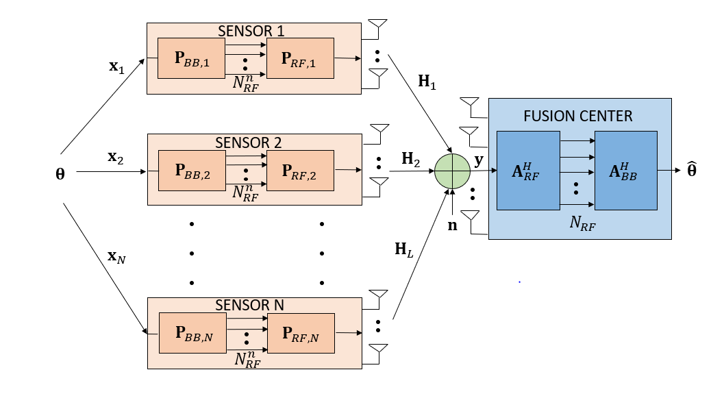
A mmWave-based MIMO IoTNe supporting IoTNos and a FC is considered as shown in Fig. 1. Each IoTNo employs transmit antennas (TAs) and RF chains, while the FC has receive antennas (RAs) and RF chains, where . The IoTNos are sensing/ monitoring a common parameter vector comprised of different physical quantities that have to be estimated. The observation vector of IoTNo , represented by can be modeled as
| (1) |
where and represent the observation matrix and the observation noise corresponding to the th IoTNo, respectively. Each node employs the hybrid TPC comprised of the cascaded BB and RF TPC matrices and , respectively. Subsequently, each IoTNo transmits its precoded observations to the FC over a coherent multiple access channel (MAC). Therefore, the signal received at the FC can be modeled as
| (2) |
where the matrix represents the MIMO channel matrix between each IoTNo and the FC, whereas the vector represents the FC noise and follows the distribution . The stacked observation matrix , concatenated channel matrix , the overall block-diagonal BB TPC and RF TPC are defined as
| (3) | ||||
| (4) | ||||
| (5) | ||||
| (6) |
At the FC, the hybrid RC operation is performed using the cascaded RF and BB combining matrices and , respectively, to yield the estimate as
| (7) |
Since, the hybrid MIMO architecture employs the constant magnitude RF TPC and RC matrices, their elements can be constrained as follows
| (8) |
Furthermore, the MIMO channel matrix is defined as [41, 6]
| (9) |
where the 3-tuple represents the complex gain , angle of arrival (AoA) at the FC, and angle of departure (AoD) at the th IoTNe associated with the th cluster and denotes the total number of clusters. The vectors and represent the array response vectors at the FC and the th IoTNo, respectively, corresponding to the th cluster, which are defined as
| (10) |
| (11) |
where and . The quantities and denote the carrier’s wavelength and inter-antenna spacings at the FC and each IoTNo, respectively. The mmWave MIMO channel can be equivalently expressed in the compact form of
| (12) |
where are termed the array response matrices corresponding to the FC and the th IoTNo, respectively, and comprises of the path-gains. We assume that the FC has perfect knowledge of the array response matrices , and the gain matrix . The next section describes our novel hybrid transceiver designed for the MSE minimization of a noiseless FC.

III Hybrid Transceiver Design for a Noiseless FC
The purpose of this study is to determine the minimum number of RF chains required at each sensor to achieve the minimum MSE. We would like to emphasize that, in this scenario, the observation noise dominates the thermal noise at the receiver, which renders the latter negligible. Thus, the measurements of each sensor are corrupted by observation noise, which necessitates the design of the hybrid TPCs. On account of a noiseless FC, the received vector can be obtained by substituting in (II). The estimate at the output of the LMMSE RC for a noiseless coherent MAC is given by
| (13) |
Furthermore, the resultant MSE at the FC, which is defined as , can be expressed as
| (14) |
Hence, we can formulate the optimization problem of our hybrid transceiver with an objective to minimize the MSE in (14) as follows
| (15) |
The constant magnitude of the elements in the RF TPC and RC results in the non-convexity of the above optimization problem, and makes it intractable. In this context, suitable RF TPCs and RC can be obtained by using the procedure outlined in the next subsection, which is followed by the design of the optimal BB TPC for each IoTNo . This section considers the variance of each parameter to be and the observation noise covariance to be .
III-A Design of RF TPCs and RC
Since the columns of the matrices and are the array response vectors corresponding to the AoAs at the FC and AoDs at the th IoTNo, the columns of the RF RC and TPC can be set using the dominant array response vectors, respectively. In order to design the RF TPC for the th IoTNo, we organise the complex gains in decreasing order of magnitude so that . The RF TPC for the th IoTNo can be designed by selecting the columns denoted by the set , which contains the indices of the dominant transmit array response vectors. This is mathematically represented as
| (16) |
The design of the RF RC is described next. Let the quantity denote the sum of the magnitudes of the complex path-gains of each IoTNo corresponding to the th cluster. One can now arrange the quantities in decreasing order of their magnitude, so that . The RF RC is obtained as
| (17) |
where we have . Employing these settings of the RF TPC and RC , the design of the optimal BB TPC for each IoTNo is described next.
III-B Baseband TPC design
Upon employing the LMMSE BB RC at the FC as shown in (13), the resultant error covariance matrix is given by
| (18) |
where we have . Furthermore, assuming that the effective channel between each IoTNo and the FC is invertible, solving the optimization problem for is equivalent to solving it for . As a result, the optimization problem in (15) can be restated as
| subject to | (19) |
The above problem can be solved using Cauchy’s interlacing theorem which is described next in detail. Let us assume that the singular value decomposition (SVD) of is given by
| (20) |
where , are unitary matrices and is the matrix containing singular values on its principal diagonal. Now, substituting the SVD of into , one obtains
| (21) |
where we have . Upon substituting the SVD of as into , we arrive at:
| (22) |
where the unitary matrix obeys . Let denote the th smallest eigenvalue of any symmetric matrix . Then it follows from (22) that
| (23) |
where represents the upper block of the matrix . By exploiting Cauchy’s interlacing theorem for the eigenvalues of a subblock matrix, we have
| (24) |
for . Therefore, upon using (23) and (24), we may conclude that
| (25) |
and , when . Hence, the MSE can be lower-bounded as
| (26) |
It follows from the above relationship that the minimum MSE is obtained when . Furthermore, observe that , hence the lower bound is achieved when , i.e., the minimum number of RF chains required is equal to the parameter dimension. This implies that the singular matrix has the following structure
| (27) |
Furthermore, in order to achieve the lower bound in (26), the inequality in (24) should be satisfied with equality. This implies that the matrix should be set as an identity matrix of dimension , which results in the relationship . Hence, the optimal matrix , denoted by , can be set as
| (28) |
where is any unitary matrix, since it does affect the MSE. Subsequently, the baseband precoder matrix for the individual sensors can be extracted using
| (29) |
where . Finally, the relationship between the MSE performance achieved and the number of RF chains used can be summarized as follows:
The next section considers the most general scenario, where both realistic observation and FC noise are present and develops the hybrid minimum-MSE transceiver design, while also taking the available transmit power at each IoTNo into account.
| (30) |
IV Hybrid Transceiver Design for a Noisy FC
Again, this section develops a novel hybrid transceiver design for the more general scenario, where realistic channel-noise is also present. Additionally, another challenging aspect is also considered, where one does not have perfect knowledge of the dominant array response matrices. Hence, in this scenario, initially an iterative algorithm is developed for designing the minimum-MSE optimal fully-digital TPCs and RC matrices. Once convergence is achieved, the fully-digital matrices are decomposed into their RF and baseband counterparts using the popular SOMP algorithm. The detailed procedure is described next. The estimate for the received vector in (II) can be obtained as
| (31) |
The expression of the resultant MSE, which denoted by , is given in (30). The average transmit power corresponding to the th IoTNo can be evaluated as
| (32) |
where represents the maximum available transmit power at the th IoTNo. Hence, the MSE-minimization optimization problem for designing the hybrid transceiver can be formulated as
| (33) |
The above optimization problem is once again non-convex due to the constant-magnitude constraint as well as the non-convex objective function. However, for designing the fully-digital transceiver, one can ignore the non-convex constant magnitude constraint. Furthermore, the block-convex nature of the objective function in terms of the TPCs at the IoTNos and RC at the FC can be exploited using the BCD-based iterative framework, which designs the minimum-MSE TPC and combiner in an iterative fashion.
Employing the BCD algorithm, the optimization framework of the fully digital RC matrix assuming that all the TPC matrices are known reduces to the unconstrained problem of
| (34) |
Since the MSE objective in (30) is a quadratic convex function in terms of the RC matrix , the optimal RC matrix can be obtained by differentiating it with respect to and equating it to zero, which is given as
| (35) |
Given the minimum-MSE fully digital RC, the TPC matrices corresponding to each IoTNo can be designed by formulating the optimization problem of
| (36) |
The above optimization problem is convex in nature for a particular TPC matrix corresponding to the th IoTNo assuming that all the TPC matrices corresponding to the other IoTNos are known in addition to the RC . Upon invoking the Karush-Kuhn-Tucker (KKT) framework [42] for the above problem, the Lagrangian function is given by
| (37) |
where is the dual variable corresponding to the th sensor’s power constraint. Upon employing the first order optimality KKT condition, the minimum-MSE TPC matrix corresponding to the th IoTNo, which is denoted by , can be obtained as
| (38) |
The optimal dual variable corresponding to each IoTNo can be obtained by solving the complementary slackness condition:
| (39) |
The calculation of dual variables is shown in Appendix A. The above iterative algorithm terminates, when either a desired MSE level is achieved or a certain pre-set number of iterations have been performed. Once, the minimum-MSE fully-digital TPCs and RC matrices are derived, the next two subsections describe the SOMP algorithm based procedure of decomposing them into their RF and BB counterparts.
IV-A SOMP based hybrid transceiver design
IV-A1 Precoder design
This subsection describes the detailed procedure of decomposing the minimum-MSE fully-digital TPC matrix corresponding to each IoTNo into its RF and BB counterparts and , respectively. The corresponding optimization problem can be readily formulated as
| (40) |
The above problem is non-convex and intractable in nature, since the elements of the RF TPC must have constant magnitude. However, one can exploit an interesting relationship between the optimal TPC and the transmit array response matrix , which is shown next in detail. It allows us to design using the columns of the . To this end, using the expression for the minimum-MSE TPC in (IV) and subsequently substituting the SVD of the matrix , one obtains
| (41) |
This implies that the column space of the TPC matrix corresponding to the th IoTNo lies in the column space of the unitary matrix . Moreover, the columns of span the row space of the channel matrix . Thus, it can be concluded that
| (42) |
It can be observed from (12) that the row-space of the mmWave MIMO channel matrix is a subset of the column-space of the transmit array response matrix . Thus, we can write
| (43) |
Hence, we can design the RF TPC matrix by extracting the columns of , which by default satisfies the constant-magnitude condition. Thus, the optimization problem of designing the BB TPC can be formulated as
| (44) | ||||
where the first constraint implies that the matrix is block-sparse in nature, since only rows out of rows are non-zero. Hence, similar to Ayach et al. [8], the simultaneous orthogonal matching pursuit (SOMP) algorithm is employed for design of the RF and BB components of the TPC, since the latter is a simultaneously sparse matrix. Algorithm-1 describes the proposed SOMP-based hybrid TPC design technique in detail. The next subsection describes the detailed procedure to decompose the minimum-MSE RC matrix into its RF and BB counterparts.
IV-A2 Combiner design
Once the optimal RF and baseband TPC matrices corresponding to each IoTNo are derived, the next objective is to decompose the minimum-MSE RC matrix into its RF and baseband counterparts. The corresponding optimization is formulated as
| (45) | ||||
Upon, ignoring the constraint in the above optimization problem, the optimal solution of the unconstrained optimization problem is the RC matrix given in (IV). As shown in [8], the above optimization problem may also be modified as
| (46) | ||||
The above problem is non-convex due to the constant-magnitude constraint. However, similar to the previous subsection, it can be shown that the column space of the RC matrix lies in the column space of the concatenated mmWave MIMO channel . The detailed justification for this follows next. The optimal fully digital RC expression given in (IV) can also be written equivalently as
| (47) |
where the block-diagonal TPC matrix is defined as
and . Substituting , and using the property , for any suitable matrices and , the optimal fully-digital RC expression above can further be recast as
| (48) |
where and . It can now be observed that any column of can be written as a linear combination of the columns of . Furthermore, the columns of the matrix are linear combinations of the columns of the receive array response matrix . Thus, it can be concluded that
| (49) |
Hence, we can design by extracting columns from , which also satisfy the constant gain condition on the elements of the RF RC matrix. Subsequently, one can develop the BB RC design problem as
| (50) | ||||
The above optimization problem is once again a sparse signal recovery problem and can be solved similar to (44) upon employing the SOMP algorithm. The complete iterative procedure of designing the hybrid transceiver is summarized in Algorithm-2. The next subsection presents a proof of the convergence of the proposed BCD-based iterative algorithm.
IV-B Convergence analysis
The proposed BCD-based iterative transceiver scheme’s theoretical convergence can be proved as follows. Due to the fact that the optimization problems of the fully-digital RC and TPC matrices in (34) and (IV) are convex in nature, the following inequalities hold:
| (51) |
Hence, is a monotonically decreasing sequence and it is lower-bounded by zero. This proves that the algorithm converges. On convergence, the SOMP algorithm is employed for obtaining the RF and BB TPCs and RCs from their respective fully-digital counterparts.
The next section develops robust transceiver designs for a scenario associated with CSI uncertainty.
V Robust Hybrid Transceiver Design for a Noisy FC
In practical scenarios, it is impossible to have perfect CSI knowledge between each IoTNo and the FC due to the limited pilot overhead and quantization errors. Hence, in a practical system, one has to take the CSI uncertainty into account. Therefore, motivated by [37, 38, 35], we model the channel between each IoTNo and the FC as
| (52) |
where denotes the available channel estimate and represents the estimation error matrix whose elements obey the distribution .


Substituting from (52) into the expression in (30), the expression for the resultant average MSE defined as , is given by
| (53) |
The detailed steps are shown in Appendix B. Hence, the pertinent optimization problem for designing the hybrid transceiver in this framework associated with CSI uncertainty so that the average MSE is minimized at the FC is similar to (IV), with the objective function replaced by . The BCD-based iterative framework can once again be employed to design the fully-digital robust transceiver followed by the SOMP algorithm to yield the robust hybrid TPC and RC matrices. One can determine the robust RC matrix at the FC for a given set of robust TPC matrices , by setting , as
| (54) |
The optimization problem of designing the robust TPC matrices, given the fully-digital RC matrix, is equivalent to (IV) with replaced by . This can be solved along similar lines by invoking the KKT framework of [42] to obtain the robust fully-digital TPC matrices, given as
| (55) |
As described in the previous section, the SOMP-based algorithm can once again be employed for deriving the hybrid TPC and RC matrices for this scenario in the face of CSI uncertainty. The next subsection derives the centralized MMSE benchmark, which acts as a lower bound for the LDE schemes.
V-A Centralized MMSE benchmark
The centralized MMSE benchmark represents the best achievable performance where all the IoTNo observations are directly available at the FC. The observation vector available at the FC can be modeled as
| (56) |
where . The MSE is formulated as
| (57) |
The MSE bound above can be used as a benchmark for the evaluation of the performance of the proposed LDE schemes. The next section discusses the simulation results to illustrate the effectiveness of the various designs proposed.
VI Simulation Results


A mmWave MIMO IoTNe is considered where each IoTNo is equipped with TAs, and the FC has RAs. The number of clusters in the mmWave MIMO channel is set to clusters. The path-gains are randomly generated from the distribution . The dimension of the parameter vector to be estimated is set to and the number of observations made by each IoTNo is set to . The observation SNR is defined as whereas the . The elements of the observation matrix have been randomly generated from the distribution .


Fig. 3(a) illustrates the MSE performance of the proposed hybrid transceiver against the number of RF chains employed at each IoTNo at dB. Observe that the MSE performance improves upon increasing the number of RF chains, and as claimed in (26) it matches the centralized MMSE benchmark derived in (57) when the number of RF chains becomes equal to the parameter length . It can also be readily observed that increasing the number of RF chains beyond the parameter dimension does not result in any improvement in the MSE performance at the FC, thus validating our analytical result.
Fig. 3(b) illustrates the MSE versus , when the number of RF chains is set equal to the length of the parameter . It can be observed from the figure that the MSE of both the proposed scheme and the centralized benchmark improve upon increasing the observation SNR, which is along expected lines. Moreover, the gap between the proposed scheme and the centralized benchmark decreases upon increasing the observation SNR and matches the centralized benchmark at high SNRs, thus validating the effectiveness of the proposed scheme.
Fig. 4(a) depicts the MSE performance as a function of the number of the BCD-iterations for the design proposed in Section-IV for a noisy FC with perfect CSI. The number of IoTNos is for this particular plot. To benchmark the SOMP-based hybrid transceiver design’s performance, its corresponding fully-digital performance has also been shown. The MSE performance improves as the number of iterations increases. Furthermore, the MSE also decreases as the number of sensors increases, a trend that is along expected lines due to the availability of a larger number of observations.
Fig. 4(b) illustrates the MSE performance against the dimension of the underlying parameter vector of interest for different number of IoTNos . Observe that the MSE performance degrades upon increasing the dimensionality of the parameter. When increasing the number of IoTNos, the MSE performance improves as it leads to the availability of more measurements of the parameter, thereby increasing the estimation accuracy. The performance of the proposed SOMP-based hybrid transceiver design is observed to be very close to that of the fully-digital transceiver design, demonstrating the efficiency of the proposed design.


Fig. 5(a) illustrates the MSE versus the number of RF chains at each IoTNo for different number of RF chains at the noisy FC. The number of IoTNos considered in the system is . Again, the MSE performance of the SOMP-based hybrid transceiver improves upon increasing the number of RF chains. It becomes equivalent to the MSE corresponding to the fully-digital design, because becomes equal to the total number of TAs . It is also observed that upon increasing the number of RF chains at the FC, the MSE performance further improves. However, for clusters, it is observed that the MSE performance of the hybrid designs becomes similar. This demonstrates that the FC is indeed capable of recovering the active beams using our SOMP-based RF RC when and there is no further improvement in performance upon increasing .
Fig. 5(b) illustrates the MSE performance of the hybrid transceiver designs versus . For comparison, a heterogeneous IoTNe is considered, where the observation noise power at each sensor takes values from the following set . This setup is compared to a homogeneous IoTNe, where the observation noise at each sensor is . The homogeneous mmWave IoTNe is observed to perform better than its counterpart if the SNR value at each IoTNo for the homogeneous mmWave IoTNe is higher than that of heterogeneous mmWave counterpart. Upon increasing the number of RAs from to , the MSE performance improves due to the array gain in the noise limited region. As increases, the performance gain due to the increasing array gain becomes negligible.
Fig. 6(a) plots the MSE as a function of for the hybrid TPC/ RC designs derived in Section-IV and Section-V, respectively. The iterative algorithm is run for 15 iterations for each value. As expected, the MSE performance improves as increases, and the robust design offers significant performance improvements over the imperfect CSI-based design that ignores the CSI uncertainty. The corresponding performance of the fully-digital transceiver is once again plotted for benchmarking the hybrid transceiver designs.
Fig. 6(b) shows the MSE performance of the hybrid transceiver designs proposed in Section-IV and Section-V, for scenarios of perfect and imperfect CSI, respectively. To benchmark the performance of the hybrid TPC/ RC designs, the MSE performance corresponding to their fully-digital counterparts is also plotted. The iterative algorithm proposed for our robust transceiver design converges in 15 iterations. It can observed from the figure that the proposed robust design offers an improved MSE performance in comparison to its uncertainty-agnostic counterpart. In addition, its performance is also close to the perfect CSI-based design, which illustrates its value for practical systems.
Fig. 7(a) compares the MSE performance of our hybrid TPC/ RC design of Section IV to that of the corresponding designs in [9] and [10] that proposed the alternating minimization (AltMin) algorithm based on manifold optimization (MO) and penalty dual decomposition (PDD), respectively. The figure clearly demonstrates that the proposed SOMP-based design outperforms both these algorithms. Similarly, Fig. 7(b) compares the MSE performance of the proposed SOMP-based robust hybrid TPC/ RC design of Section V with that of [9] and [10], considering both perfect CSI and CSI-uncertainty agnostic approaches. It can be deduced from the figure that the proposed robust design offers a significant MSE performance improvement over both the agnostic as well as perfect CSI-based hybrid designs of [9] and [10]. This illustrates the efficacy of our proposed robust design.
Fig. 8 shows the MSE performance versus the number of IoTNos in the network for the schemes proposed in Section-IV and -V, both with perfect and imperfect CSI, respectively. As expected, the MSE decreases upon increasing the number of sensors, which reinforces the trend seen in the previous figures.
VII Conclusion
Hybrid transceiver designs were conceived for the LDE of a parameter vector in a mmWave MIMO IoTNe. Separate design procedures were presented for a noiseless as well as noisy FC. An important observation for the proposed hybrid transceiver design for a noiseless FC is that even in systems having a large number of antennas both at the IoTNos and the FC, increasing the number of RF chains beyond the parameter dimension does not result in any further MSE improvement. For a noisy FC, the fully digital TPC/ RC are initially determined using a BCD-based iterative framework followed by the SOMP technique for decomposing it into its RF and BB components. A robust hybrid design procedure was also formulated for a practical scenario having CSI uncertainty, which provides improved estimation performance over its CSI uncertainty-agnostic counterpart. Our simulation results illustrate the performance of the proposed schemes and corroborate our analytical findings.
Appendix A Calculation of dual variables
To obtain the dual variable at the th IoTNo, let the following matrices be defined as
| (59) | ||||
| (60) |
where and . The minimum-MSE TPC matrix in (IV) can be compactly written as
| (61) |
Since is a Hermitian symmetric matrix, its eigenvalue decomposition (EVD) is given by . Initially, is calculated by setting . If the average transmit power in (IV) is satisfied, then . Otherwise for a non-zero dual variable, the average transmit power is met with equality from the complementary slackness condition
| (62) |
The value of the dual variable for the average transmit power to be satisfied with equality can be calculated as
| (63) | ||||
where is the th eigenvalue of and is the th element of matrix . The dual variable can now be obtained via the classic bisection method.
Appendix B Average MSE calculation in (V)
The channel estimation error matrices for each IoTNo in (52) are assumed to be independent of each other. The average MSE is given by (VII) shown at the top of this page.
The lemma described below is employed to evaluate the average MSE.
Lemma 1.
Consider a matrix , defined as , where is known and each element of is assumed to be Gaussian distributed as . Then, for a matrix , the following properties hold
Proof.
The first result of Lemma 1 can be proved as follows: The term can be expanded as
| (64) |
For compact representation, consider and as shown above.
Each element of is the dot product of the row of and column of . This implies that
Thus, the expected value of any element of is zero, since . This further implies that
Following the same reasoning as above, it can be shown that
To compute the expected value of , let us denote the EVD of the Hermitian matrix as . Therefore, we have
where , whose elements are also distributed as since is a unitary matrix. Thus, the above expression can be simplified as follows:
where denotes the column of . Upon assuming that all the elements of are independent and identically distributed, , we have
From the above results and (B), we conclude that
Hence, the first result of Lemma 1 is proved.
The next result of the lemma can be proven by expanding the quantity as
| (65) |
As explained previously, the expected value of the second and third terms above is equal to zero. The expected value of the fourth term is given by
where (a) follows from the fact that and are independent of each other. This implies that
which proves the second result of Lemma 1. ∎
References
- [1] S. Andreev, C. Dobre, and P. Misra, “Internet of things and sensor networks,” IEEE Communications Magazine, vol. 58, no. 4, pp. 74–74, 2020.
- [2] N. Ahmed, D. De, and I. Hussain, “Internet of things (IoT) for smart precision agriculture and farming in rural areas,” IEEE Internet of Things Journal, vol. 5, no. 6, pp. 4890–4899, 2018.
- [3] H. Harb, A. Mansour, A. Nasser, E. M. Cruz, and I. de la Torre Díez, “A sensor-based data analytics for patient monitoring in connected healthcare applications,” IEEE Sensors Journal, vol. 21, no. 2, pp. 974–984, 2021.
- [4] M. Carminati, O. Kanoun, S. L. Ullo, and S. Marcuccio, “Prospects of distributed wireless sensor networks for urban environmental monitoring,” IEEE Aerospace and Electronic Systems Magazine, vol. 34, no. 6, pp. 44–52, 2019.
- [5] O. Cetinkaya, D. Balsamo, and G. V. Merrett, “Internet of MIMO things: UAV-assisted wireless-powered networks for future smart cities,” IEEE Internet of Things Magazine, vol. 3, no. 1, pp. 8–13, 2020.
- [6] R. W. Heath, N. Gonzalez-Prelcic, S. Rangan, W. Roh, and A. M. Sayeed, “An overview of signal processing techniques for millimeter wave MIMO systems,” IEEE Journal of Selected Topics in Signal Processing, vol. 10, no. 3, pp. 436–453, 2016.
- [7] A. F. Molisch, V. V. Ratnam, S. Han, Z. Li, S. L. H. Nguyen, L. Li, and K. Haneda, “Hybrid beamforming for massive MIMO: A survey,” IEEE Communications Magazine, vol. 55, no. 9, pp. 134–141, 2017.
- [8] O. El Ayach, S. Rajagopal, S. Abu-Surra, Z. Pi, and R. W. Heath, “Spatially sparse precoding in millimeter wave MIMO systems,” IEEE Transactions on Wireless Communications, vol. 13, no. 3, pp. 1499–1513, 2014.
- [9] X. Yu, J.-C. Shen, J. Zhang, and K. B. Letaief, “Alternating minimization algorithms for hybrid precoding in millimeter wave MIMO systems,” IEEE Journal of Selected Topics in Signal Processing, vol. 10, no. 3, pp. 485–500, 2016.
- [10] Q. Shi and M. Hong, “Spectral efficiency optimization for millimeter wave multiuser MIMO systems,” IEEE Journal of Selected Topics in Signal Processing, vol. 12, no. 3, pp. 455–468, 2018.
- [11] J.-J. Xiao, S. Cui, Z.-Q. Luo, and A. J. Goldsmith, “Linear coherent decentralized estimation,” IEEE Transactions on Signal Processing, vol. 56, no. 2, pp. 757–770, 2008.
- [12] A. S. Behbahani, A. M. Eltawil, and H. Jafarkhani, “Linear decentralized estimation of correlated data for power-constrained wireless sensor networks,” IEEE Transactions on Signal Processing, vol. 60, no. 11, pp. 6003–6016, 2012.
- [13] N. K. D. Venkategowda and A. K. Jagannatham, “Optimal minimum variance distortionless precoding (MVDP) for decentralized estimation in MIMO wireless sensor networks,” IEEE Signal Processing Letters, vol. 22, no. 6, pp. 696–700, 2015.
- [14] K. P. Rajput, Y. Verma, N. K. D. Venkategowda, A. K. Jagannatham, and P. K. Varshney, “Linear MMSE precoder combiner designs for decentralized estimation in wireless sensor networks,” in GLOBECOM 2020 - 2020 IEEE Global Communications Conference, 2020, pp. 1–6.
- [15] Q. Zhou, D. Li, S. Kar, L. M. Huie, H. V. Poor, and S. Cui, “Learning-based distributed detection-estimation in sensor networks with unknown sensor defects,” IEEE Transactions on Signal Processing, vol. 65, no. 1, pp. 130–145, 2017.
- [16] V. Gupta and S. De, “An energy-efficient edge computing framework for decentralized sensing in WSN-Assisted IoT,” IEEE Transactions on Wireless Communications, vol. 20, no. 8, pp. 4811–4827, 2021.
- [17] A. S. Leong, S. Dey, and J. S. Evans, “Asymptotics and power allocation for state estimation over fading channels,” IEEE Transactions on Aerospace and Electronic Systems, vol. 47, no. 1, pp. 611–633, 2011.
- [18] A. S. Leong, S. Dey, G. N. Nair, and P. Sharma, “Power allocation for outage minimization in state estimation over fading channels,” IEEE Transactions on Signal Processing, vol. 59, no. 7, pp. 3382–3397, 2011.
- [19] J. Akhtar and K. Rajawat, “Distributed sequential estimation in wireless sensor networks,” IEEE Transactions on Wireless Communications, vol. 17, no. 1, pp. 86–100, 2017.
- [20] X. Cheng, P. Khanduri, B. Chen, and P. K. Varshney, “Joint collaboration and compression design for distributed sequential estimation in a wireless sensor network,” IEEE Transactions on Signal Processing, vol. 69, pp. 5448–5462, 2021.
- [21] N. K. D. Venkategowda, H. Lee, and I. Lee, “Joint transceiver designs for MSE minimization in MIMO wireless powered sensor networks,” IEEE Transactions on Wireless Communications, vol. 17, no. 8, pp. 5120–5131, 2018.
- [22] N. K. Venkategowda, H. Lee, and I. Lee, “Data precoding and energy transmission for parameter estimation in mimo wireless powered sensor networks,” in 2017 IEEE 86th Vehicular Technology Conference (VTC-Fall). IEEE, 2017, pp. 1–5.
- [23] Z. Zhu, Z. Wang, Y. Lin, P. Liu, W. Hao, Z. Wang, and I. Lee, “Robust max-min fair beamforming of secrecy SWIPT IoT systems under a non-linear EH model,” in 2021 IEEE International Conference on Communications Workshops (ICC Workshops), 2021, pp. 1–6.
- [24] F. Jiang, J. Chen, A. L. Swindlehurst, and J. A. López-Salcedo, “Massive MIMO for wireless sensing with a coherent multiple access channel,” IEEE Transactions on Signal Processing, vol. 63, no. 12, pp. 3005–3017, 2015.
- [25] A. Shirazinia, S. Dey, D. Ciuonzo, and P. Salvo Rossi, “Massive MIMO for decentralized estimation of a correlated source,” IEEE Transactions on Signal Processing, vol. 64, no. 10, pp. 2499–2512, 2016.
- [26] D. Ciuonzo, P. S. Rossi, and S. Dey, “Massive MIMO channel-aware decision fusion,” IEEE Transactions on Signal Processing, vol. 63, no. 3, pp. 604–619, 2015.
- [27] Y. Liu and C. Li, “Secure distributed estimation over wireless sensor networks under attacks,” IEEE Transactions on Aerospace and Electronic Systems, vol. 54, no. 4, pp. 1815–1831, 2018.
- [28] H. Liu, S. Wang, X. Zhao, S. Gong, N. Zhao, and T. Q. Quek, “Analog–digital hybrid transceiver optimization for data aggregation in IoT networks,” IEEE Internet of Things Journal, vol. 7, no. 11, pp. 11 262–11 275, 2020.
- [29] H. Liu, S. Wang, S. Gong, N. Zhao, J. An, and T. Q. S. Quek, “Hybrid LMMSE transceiver optimization for distributed IoT sensing networks with different levels of synchronization,” IEEE Internet of Things Journal, vol. 8, no. 19, pp. 14 458–14 470, 2021.
- [30] S. H. Chae, C. Jeong, and S. H. Lim, “Simultaneous wireless information and power transfer for Internet of Things sensor networks,” IEEE Internet of Things Journal, vol. 5, no. 4, pp. 2829–2843, 2018.
- [31] K. P. Rajput, A. Kumar, S. Srivastava, A. K. Jagannatham, and L. Hanzo, “Bayesian learning-based linear decentralized sparse parameter estimation in MIMO wireless sensor networks relying on imperfect CSI,” IEEE Transactions on Communications, vol. 69, no. 9, pp. 6236–6250, 2021.
- [32] K. P. Rajput, M. F. Ahmed, N. K. D. Venkategowda, A. K. Jagannatham, G. Sharma, and L. Hanzo, “Robust decentralized and distributed estimation of a correlated parameter vector in MIMO-OFDM wireless sensor networks,” IEEE Transactions on Communications, vol. 69, no. 10, pp. 6894–6908, 2021.
- [33] N. K. D. Venkategowda, B. B. Narayana, and A. K. Jagannatham, “Precoding for robust decentralized estimation in coherent-MAC-based wireless sensor networks,” IEEE Signal Processing Letters, vol. 24, no. 2, pp. 240–244, 2017.
- [34] H. Rostami and A. Falahati, “Precoder design for decentralised estimation over MIMO-WSN based on stochastic models,” IET Communications, vol. 12, no. 6, pp. 736–742, 2018.
- [35] K. Xu, Y. Cai, M. Zhao, Y. Niu, and L. Hanzo, “MIMO-aided nonlinear hybrid transceiver design for multiuser mmwave systems relying on Tomlinson-Harashima precoding,” IEEE Transactions on Vehicular Technology, vol. 70, no. 7, pp. 6943–6957, 2021.
- [36] L. Jiang and H. Jafarkhani, “MmWave amplify-and-forward MIMO relay networks with hybrid precoding/combining design,” IEEE Transactions on Wireless Communications, vol. 19, no. 2, pp. 1333–1346, 2019.
- [37] Y. Cai, Y. Xu, Q. Shi, B. Champagne, and L. Hanzo, “Robust joint hybrid transceiver design for millimeter wave full-duplex MIMO relay systems,” IEEE Transactions on Wireless Communications, vol. 18, no. 2, pp. 1199–1215, 2019.
- [38] M.-M. Zhao, Y. Cai, M.-J. Zhao, Y. Xu, and L. Hanzo, “Robust joint hybrid analog-digital transceiver design for full-duplex mmwave multicell systems,” IEEE Transactions on Communications, vol. 68, no. 8, pp. 4788–4802, 2020.
- [39] C. Wang, Z. Li, T.-X. Zheng, H. Chen, and X.-G. Xia, “Robust hybrid precoding design for securing millimeter-wave IoT networks under secrecy outage constraint,” IEEE Internet of Things Journal, vol. 8, no. 16, pp. 13 024–13 038, 2021.
- [40] K. P. Rajput, S. Srivastava, R. Akarapu, P. Maity, and A. K. Jagannatham, “Hybrid precoder designs for decentralized parameter estimation in millimeter wave (mmWave) sensor networks with perfect and imperfect CSI,” Physical Communication, vol. 47, p. 101377, 2021.
- [41] D. Tse and P. Viswanath, Fundamentals of Wireless Communication. Cambridge university press, 2005.
- [42] S. Boyd and L. Vandenberghe, Convex optimization. Cambridge university press, 2004.