Motion Planning (In)feasibility Detection using a Prior Roadmap via Path and Cut Search
Abstract
Motion planning seeks a collision-free path in a configuration space (C-space), representing all possible robot configurations in the environment. As it is challenging to construct a C-space explicitly for a high-dimensional robot, we generally build a graph structure called a roadmap, a discrete approximation of a complex continuous C-space, to reason about connectivity. Checking collision-free connectivity in the roadmap requires expensive edge-evaluation computations, and thus, reducing the number of evaluations has become a significant research objective. However, in practice, we often face infeasible problems: those in which there is no collision-free path in the roadmap between the start and the goal locations. Existing studies often overlook the possibility of infeasibility, becoming highly inefficient by performing many edge evaluations.
In this work, we address this oversight in scenarios where a prior roadmap is available; that is, the edges of the roadmap contain the probability of being a collision-free edge learned from past experience. To this end, we propose an algorithm called iterative path and cut finding (IPC) that iteratively searches for a path and a cut in a prior roadmap to detect infeasibility while reducing expensive edge evaluations as much as possible. We further improve the efficiency of IPC by introducing a second algorithm, iterative decomposition and path and cut finding (IDPC), that leverages the fact that cut-finding algorithms partition the roadmap into smaller subgraphs. We analyze the theoretical properties of IPC and IDPC, such as completeness and computational complexity, and evaluate their performance in terms of completion time and the number of edge evaluations in large-scale simulations.
I Introduction
Motion planning [1] is a crucial functionality for autonomous robots that enables them to move from one configuration to another without colliding with obstacles. The main objective of most motion planing algorithms is efficiency, that is, finding a solution as quickly as possible.
Most existing algorithms start from the assumption that a successful motion plan exists, only terminating with failure after exhaustively searching the plan space or exceeding a time budget [2, 3, 4, 5, 6, 7, 8, 9]. However, in practical settings, it may not be uncommon for planning problems to be infeasible. For example, it may be impossible to grasp an object due to nearby objects blocking the way or the robot’s kinematic limitations. The prospect of plan infeasibility is particularly salient in task and motion planning [10, 11], where many motion planning subproblems are considered. In this paper, we address the problem of detecting infeasibility (while still efficiently finding a solution when one exists), particularly in scenarios where learning from past experience is available.

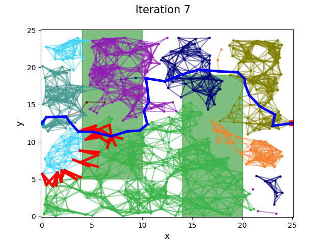
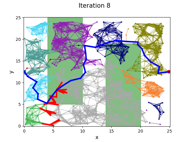
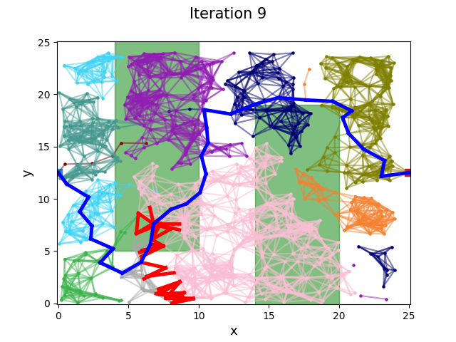
Specifically, we focus on Step 2 of a three-step learning-based framework for obtaining motion plans (or determining their non-existence) from past experience. In Step 1 of this overall framework, a representative roadmap [12, 13] is learned from available training problems. This roadmap is a graph that approximately captures connectivity in the configuration space (C-space [14]) as depicted in Figure 1. Roadmaps are widely used in motion planning, such as sampling-based motion planners [15, 16, 17, 18] which construct a roadmap to discretize a C-space and search-based planners [19] which generate a grid map corresponding to a roadmap. In Step 2, when presented with a query problem, we attempt to find a solution using the roadmap from Step 1, or alternatively to determine that no solution exists (i.e., infeasibility in the roadmap). In Step 3, if a solution has been found in Step 2, its quality is refined. On the other hand, if no solution was found, an attempt is made to prove infeasibility in the continuous C-space. Alternatively, points can be added to the roadmap from Step 1 to make it denser before repeating Step 2. In this work, we specifically concentrate on Step 2 by assuming the existence of a roadmap from Step 1, and we leave Step 3 for future work.
Roadmaps are a useful data structure for accumulating past planning results. Edges in a roadmap are hypothesized to be collision-free paths between their endpoints. However, they may not actually be collision-free in the real world; in practice, they must be evaluated by a motion planner to check for collisions. We can exploit past experience to obtain the probability of local connectivity between vertices in a roadmap (i.e., their connecting edge being collision-free) and use the roadmap as prior knowledge to solve a query problem.
One possible approach to obtaining connection probabilities is to use the counting principle. Given training problems that may be either feasible or infeasible, whose C-spaces vary due to various numbers, shapes, and locations of obstacles, we generate a single representative roadmap by attempting to solve them with a given motion planner. Then, for each edge in the roadmap, we count the number of problems that the edge is confirmed collision-free out of the total number of problems; we apply the same procedure for all edges to form their existence probabilities. It is important to note that our method also works in cases where there is no prior knowledge, and in such cases, all edge connection probabilities are set to (see Section IV-A).
Previous studies [20, 21, 22] have leveraged prior roadmaps to find the shortest path between nodes. Their focus is on reducing the number of edge evaluations since edge evaluation is known to consume most of the computation time in motion planning due to its expensive collision-checking procedures [23, 24, 25, 26]. However, their methods assume that a prior roadmap always contains a solution, resulting in an ineffective approach to dealing with infeasible problems. The search space of previous work is mostly a space of paths or edges; therefore, infeasible problems can only be determined after evaluating all possible paths or combinations of edges.
To detect infeasibility from a prior roadmap, we propose a different search strategy, namely iterative search over a path space and a cut space. Our insight is that the search over both spaces can identify whether a given problem is feasible efficiently, whereas trying to find a path in an infeasible problem or trying to find a cut in a feasible problem requires exploring the entire search space.
Furthermore, the result of a single path search execution can help guide the search for a cut and vice versa. We apply edge evaluations to edges found by the path search and then determine their ground-truth existence. Some edges may be identified as non-existing (i.e., colliding with obstacles), which can be leveraged by the cut search since a ground-truth cut must contain one of those non-existing edges. Similarly, a ground-truth path must include one of the existing edges identified by the cut search.
Based on this observation, we design a complete search algorithm that identifies feasibility of a given problem. We also propose a divide-and-conquer algorithm that further improves efficiency by exploiting an abstract graph data structure over a roadmap.
Our algorithms can complement existing methods by acting as preprocessors so that infeasible problems are identified as quickly as possible. If a given problem is confirmed feasible, we switch to existing approaches to find the shortest path.
In summary, we make three main contributions in this paper.
- •
We introduce two probabilistic roadmap-based algorithms that perform path and cut searches to determine whether a query problem is feasible efficiently.
- •
We analyze both algorithms’ completeness and computational complexity.
- •
We empirically verify the performance of our methods through extensive simulations.
II Problem Description
Let be a weighted graph representing a prior roadmap learned from past experience.
- •
is a vertex set. Each vertex corresponds to a robot configuration in the C-space.
- •
is an edge set whose element is denoted by .
- •
represents a Bernoulli probability of edge existence over all edges. Edge existence implies that the robot can traverse from one vertex to another without colliding with obstacles. A ground-truth edge existence can only be revealed by applying edge evaluation. indicates that the edge is known with certainty to exist, whereas indicates that the edge is known not to exist. indicates that the edge needs to be evaluated to determine whether the path from vertex to vertex is collision-free.
Start and goal configurations ( and ) are given at query time, which can be connected to near vertices in if edge evaluation guarantees no collisions; this is a typical process for multi-query planners, such as PRM [27]. For those two new edges connecting and to , . For notational convenience, we treat the enlarged roadmap the same as , including and .
The objective of the feasibility detection problem is to determine whether a collision-free path connecting and exists in (and if so, to identify such a path) while minimizing the number of edge evaluations as much as possible.
III Algorithms
In this section, we propose an algorithm (IPC) that iteratively searches over the path and cut spaces to detect feasibility. We then present another algorithm (IDPC) based on IPC that effectively decomposes the search space to improve efficiency further.
III-A Iterative path and cut finding (IPC)
Since all we care about from is connectivity between a start and a goal vertex, we treat the edge-evaluation process as a black box computation. Any information on the configuration space in which is embedded is irrelevant to the algorithm design; our algorithms are agnostic to configuration values and their dimension. We thus focus only on the graph structure of in designing algorithms.
Our idea is to leverage existing off-the-shelf path-finding and cut-finding algorithms, both highly efficient due to the long history of their individual developments. A path-finding algorithm is used to certify connectivity in , while a cut-finding algorithm confirms disconnectivity. We obtain the most probable path and cut as candidates from those algorithms and apply edge evaluations to check their ground-truth existence.11 1 In the rest of the paper, we denote the output of a pathfinding or cut-finding algorithm as a candidate path or cut, as their ground-truth existence has not yet been confirmed, and a ground-truth path or cut as simply a path or cut.


As such, we propose an algorithm to determine the feasibility of a given problem through the path and cut search in without requiring too many edge evaluations, which we call IPC. IPC iteratively applies path-finding and cut-finding algorithms while the result of one informs the search for another in the next iteration and terminates when either a path or a cut is found. Figure 2 illustrates both scenarios.
Since is a positively weighted graph, we use Dijkstra’s algorithm to find the most probable candidate path, a finite sequence of edges . To find the most probable candidate cut, a finite edge set ,22 2 Off-the-shelf minimum cut algorithms generally do not output a sequence of edges but an edge set instead, since as illustrated in Figure 2 (b), edges in a cut need not be adjacent. we adopt the Push–relabel algorithm [28] with its state-of-the-art efficiency. We present the time complexity of existing cut-finding algorithms in Table I.
| Algorithms | Complexity |
|---|---|
| Ford–Fulkerson algorithm [29] | |
| Edmond–Karp algorithm [30] | |
| Push–relabel algorithm [28] |
We initialize edge values over using . Both Dijkstra’s and the Push–relabel algorithms reason over the sum of edge values, whereas finding the most probable candidate path or cut requires reasoning over the product of probabilities. To correct this mismatch, our algorithms reason over logarithmic values. Moreover, a path-finding algorithm seeks high values, while a cut-finding algorithm prefers low values. In the end, we augment with the weight and capacity used for finding a candidate path and cut, respectively.33 3 Weight and capacity are terminologies for edge values used in the path-finding and cut-finding literature, respectively. We denote the augmented graph by , where and are weight and capacity values over such that . For , we compute and as follows.
Deterministic edges with values of or do not need evaluations. To handle those edges, we set and when and and when . The value of is used to ensure that edges with this value will not be chosen as a part of the candidate path or cut. By doing so, we ensure that if a path exists, it must pass through (at least) one of the edges identified as existing by cut finding and that if a cut exists, it must contain (at least) one of the edges identified as non-existing by pathfinding.
The pseudo-code of IPC is included in Algorithm 1. Dijkstra’s algorithm (line ) and the Push–relabel algorithm (line ) are iteratively applied. In lines and , EvaluateEdgeExistence performs edge evaluations on every edge in or and returns true if a path or cut is found. EvaluateEdgeExistence also updates and values depending on whether corresponding edges are in-collision (updating to and to ) or collision-free (updating to and to ).
A candidate path found may contain multiple collision edges, and at least one of those edges must be a part of any cut (if a cut exists). Then, the cut-finding algorithm searches for a candidate cut that includes one of these edges. We observe that choosing a center edge from the largest sequence of consecutive collision edges performs well in practice. We set for the chosen edge from to be while setting for the rest of the edges from to be (line 6), ensuring that a candidate cut must contain the chosen edge to disconnect . After confirming that a candidate cut found is not a cut, we reset the values of the other collision edges from back to for the next iteration (line 11). One may also apply a similar strategy to pathfinding by heuristically selecting one particular edge from . However, it is more complex because consists of an unordered set of edges that are not necessarily adjacent (as can be seen in Figure 2 (b)). We leave full specification of such optimization to future work; pathfinding in Algorithm 1 is applied over the entire graph.
Completeness: IPC is guaranteed to terminate by finding either a path or a cut.
Theorem 1
IPC is complete.
Proof:
Note again that pathfinding and cut-finding applications reveal the ground-truth existence of edges. Thus, if IPC can evaluate all edges in before termination without missing some edges or resulting in an infinite loop, the feasibility of a given problem can be known. After edge evaluation, the values of and will become either or . Those edges from and assigned to the value of will not be chosen by pathfinding or cut finding; both algorithms always explore new edges that have not yet been evaluated. Since has a finite number of edges, IPC will eventually evaluate all edges in the worst case. When the ground-truth existence of all edges is known, must contain either a path or a cut. Thus, one of them is guaranteed to be found. ∎
The same guarantee also holds in the continuous C-space when , as a roadmap is a discrete approximation. Counterparts of a path and cut in the continuous C-space are a one-dimensional curve and ()-dimensional hyperplane when the ambient C-space is -dimensional. If a connected curve from a start and goal exists, all hyperplanes meeting the curve must have at least one hole; otherwise, there cannot be a connected curve.
If is finite, the infeasibility proof provided by Theorem 1 is valid only for the roadmap. Step 3 of the learning framework introduced in Section I aims to convert cut edges into ()-dimensional hyperplanes to ensure infeasibility in the continuous C-space. The method [37] can be invoked in this step to learn a separating hyperplane that disconnects the start and goal.

Complexity: In IPC, the majority of computation occurs in finding a candidate cut (i.e., of Push–relabel). Figure 3 shows the time comparison of Dijkstra’s and the Push–relabel algorithms as the number of vertices and edges in increases. We observe that the time taken for cut finding dominates that for pathfinding.
Motivated by this observation, we propose an improved algorithm over IPC in the next subsection, which decomposes into smaller subgraphs so that the search space for cut finding becomes smaller. Since pathfinding computation is relatively cheap, we also present in Appendix -D the performance of IPC when increasing the number of pathfinding executions in each iteration.
III-B Iterative decomposition and path and cut finding (IDPC)
For the second algorithm, we exploit the fact that a candidate cut splits into two separate induced subgraphs44 4 An induced subgraph is a special case of a subgraph, which satisfies not only that its vertices are a subset of vertices in but also that it must contain all edges that exist in whose both endpoint vertices exist in the induced subgraph. that can be connected by some of the edges from the candidate cut if they are found to be collision-free (see Figure 4) and that the two induced subgraphs can be obtained for free as a byproduct of executing the cut-finding algorithm. For convenience, we refer to induced subgraphs as subgraphs. We search for local candidate cuts from individual subgraphs to determine their disconnectivity, further splitting them into even smaller subgraphs. Meanwhile, we aggregate this local information to determine global disconnectivity between the start and goal. Consequently, the cut-finding algorithm runs on a smaller graph instead of . We call this version iterative decomposition and path and cut finding (IDPC). Since IDPC iteratively decomposes into multiple subgraphs and composes the results of local cut findings, it can be seen as a divide-and-conquer approach.


In IDPC, the search space for a path is whereas that for a cut is a set of connected components (i.e., subgraphs). We denote the set of subgraphs by , where . Subgraph edges satisfy the two conditions and , as illustrated in Figure 5. The cut-finding algorithm identifies connecting edges between subgraphs, and we only keep collision-free connecting edges in IDPC, denoted by . Notice that when is split into and by , endpoint vertices of in form subgoals for , that is, any candidate paths must pass (at least) one of subgoals to reach . Similarly, endpoint vertices of in form substarts for . As IDPC iteratively applies cut findings, any arbitrary subgraph will contain substarts and subgoals unless completely disconnected from neighboring subgraphs. Due to the different search spaces for path and cut, the termination condition for declaring path existence is the same as in IPC, but we need another method for cut existence.

For this purpose, we introduce an abstract graph , an undirected unweighted graph used for finding a cut in from a set of cuts in . ignores the detailed structure within but captures the connectivity among through and the pairwise relationships among substarts and subgoals (Figure 6). must contain correspondence information concerning ; thus, we define as a tuple of as follows.
- •
is an abstract vertex set, where , corresponding to substarts and subgoals induced by and and in . satisfies that . In practice, .
- •
is an abstract edge set, where . Each makes one of three types of connections: (1) candidate connections between substarts and subgoals in the same ; (2) confirmed connections between substarts of and subgoals of enabled by ; (3) candidate connections among substarts or subgoals in the same . Candidate connections are those whose ground-truth connectivity has yet to be discovered. If any of the above candidate connections are identified by cut finding to be disconnected in , we do not maintain .
- •
is a Boolean function, which maps to true if a path between endpoint vertices of has been identified in or false otherwise, implying that a path may still exist.
- •
maps in to in from which is induced.
- •
maps to an index of to which belongs.
- •
is a Boolean function, which classifies the type of into either substart or subgoal. , and .
Although , is not a subgraph of because . The reason for introducing the third type of abstract edge (i.e., blue edges in Figure 6) is to cover the cases where the only feasible path visits the same subgraph multiple times by coming in and going out from a neighboring subgraph; without considering this case, IDPC is not complete.
ReflectPathEvaluation 9
ClusterSubstartsAndSubgoals 12
SubgraphPartition 15
With this new data structure, we now describe the pseudo-code of IDPC in Algorithm 2. The backbone of IDPC is similar to IPC, but it additionally includes and to reduce the search space for expensive cut finding. As initialization (lines 1 and 2), IDPC starts with a single subgraph equal to and consisting of two vertices (i.e., and ) and a single edge connecting them. We also set .
The process of searching for a candidate path is the same as IPC (lines 4-7). The result of edge evaluations over is used to update , assigning the values of and to either or , depending on the collision status (line 8). If any portion of is a collision-free subpath (i.e., a collision-free path from a substart to a subgoal in a subgraph), IDPC sets the values of for the corresponding abstract edges in to true. In line 9, IDPC chooses one subgraph out of to apply the cut-finding algorithm. In our experiments, we use a heuristic criterion to choose a subgraph that includes the largest number of collision edges in . IDPC uses the same method as in IPC for selecting a particular edge used for a candidate cut within (line 10).

Unlike which has a single start and a single goal, may have multiple substarts and subgoals, making cut-finding algorithms inapplicable, since they can only accept one pair. Also, for the candidate connections between pairs of substart and subgoal (i.e., the first type of abstract edges), it is desirable if a single cut-finding execution identifies as many disconnections between pairs as possible rather than focusing on a single pair. Notice that the more disconnections between pairs are identified, the more balanced partition will likely be made in compared to a partition obtained by trying to confirm the disconnection between a single pair. Neither method violates completeness, but the latter will likely incur more cut-finding executions, decreasing efficiency.
To handle the inapplicability issue and to encourage balanced cuts, we cluster substarts and subgoals in with dummy start and goal vertices ( and ), as shown in Figure 7, and use dummy vertices as input to cut finding (line 11). By setting the values of of edges connecting to dummy vertices to , we assure that a candidate cut can only be found within . One important point is that IDPC does not connect dummy vertices to a pair of substart and subgoal whose corresponding abstract edge in satisfies that . In Figure 7, a collision-free path colored in blue from to shows such a case; no cuts can separate from , and thus, we leave them out of candidate-cut consideration. IDPC searches for a candidate cut within in line 12 and applies the same edge value reset process as in IPC in line 13. IDPC then removes dummy vertices and edges from .


In line 14, IDPC splits into and , followed by updating accordingly. Figure 8 illustrates the subgraph partition process, where a candidate cut found is . After splitting into two, IDPC applies edge evaluations to and leaves collision-free edges. To update , IDPC executes the following three steps. First, IDPC removes the first type of abstract edges (i.e., green edges in Figure 8 (a)) and some of the third type of abstract edges (i.e., blue edges in Figure 8 (a)) if splits endpoint vertices into different partitions. Second, IDPC adds new abstract vertices from collision-free edges that exist in . Third, IDPC adds three types of new abstract edges (i.e., green and orange edges and blue edges among newly added abstract vertices in Figure 8 (b)). Function values of , , and are assigned for the new abstract vertices and edges. For , the second type of edges (i.e., orange edges in Figure 8) is initialized with true as their connectivity has already been confirmed, but the other two types are initialized to false.
Remember that the point of introducing is to check for global disconnectivity from a set of cuts discovered from previous iterations (lines 15-17). Since is an undirected unweighted graph, IDPC employs breadth-first search to to check the connectivity between abstract vertices corresponding to a start and a goal. Therefore, the termination condition for cut finding is the detection of disconnectivity in .
IDPC iterates the while loop until it finds either a path or a cut. Notice that all the computations regarding cut finding are now local. In Appendix -E, we include the pseudo-code for the remaining functions in Algorithm 2. In Appendix -F, we show a pictorial example of how IDPC operates on a small toy roadmap.
III-C Analysis
We analyze the completeness guarantee and time complexity of IDPC. The following theorem shows that the abstract graph and subgraphs still capture all possible paths and cuts by construction to preserve completeness. Therefore, like IPC, IDPC always finds a path if a given problem is feasible or a cut otherwise.
Theorem 2
IDPC is complete.
Proof:
The proof is included in Appendix -A. ∎
To analyze the time complexity of IDPC, we consider four variables: , , , and , where and are used for , whereas and are used for . Note that in the worst case, where every vertex in forms an individual subgraph, and . However, this case rarely occurs in practice, and generally, and .
| Components | Complexity |
|---|---|
| ExecutePathfinding (i.e., Dijkstra) | |
| ReflectPathEvaluation | |
| ChooseSubgraph | |
| ClusterSubstartsAndSubgoals | |
| ExecuteCutFinding (i.e., Push–relabel) | |
| SubgraphPartition |
Table II shows the complexity of major computations in Algorithm 2, which can be derived from the pseudo-code in Appendix -E. Like in IPC, the cut finding by Push–relabel dominates the overall computation. However, the cut-finding computation now applies to a subgraph whose size is and , not the entire graph as in the case of IPC, thus improving its efficiency. We achieve this improvement by embracing additional computations (as shown in Table II). To verify that those computations are relatively inconsequential, in Appendix -B, we analyze the time taken by major components of IDPC as a function of graph size.
IV Evaluation


In this section, we validate our methods by the following set of evaluations. First, we show the comparison analysis against baselines in two-dimensional C space in terms of the completion time and the number of edge evaluations. Second, we conduct more realistic simulations where a C-space is high-dimensional. We report additional evaluations in the appendix, including an analysis of the computational overhead of IDPC compared to IPC (Appendix -B), how underlying graph topologies affect performance (Appendix -C), and the performance evaluation when increasing the number of pathfinding executions at each iteration (Appendix -D).
All experiments are conducted on an Intel Core i7-8665U CPU at 1.90 GHz with 16 GB of RAM. We adopt Dijkstra’s and the Push–relabel algorithms implemented in NetworkX [31]. All plots in this section show the mean and confidence interval obtained from multiple runs.
IV-A Comparison with baselines
We evaluate algorithms in terms of the number of edge evaluations and the time taken to detect feasibility. We do not include the edge evaluation time in the total computation time because it may differ depending on the local planning method, collision-checking algorithm used, robot shape, and how much approximation of the mesh shape is considered.
We compare against three baselines: (1) applying pathfinding only (i.e., Dijkstra’s), (2) applying cut finding only (i.e., Push–relabel), and (3) the breadth-first search (BFS) based method. The first two baselines are used to show the consequence of neglecting to consider either the feasibility or infeasibility of a given problem. In particular, most existing methods in the literature that rely on the roadmap [20, 21, 22] are represented by the first baseline since infeasibility is often overlooked. Other learning-based methods that are not based on the roadmap (referred to in Section V) are omitted, as they do not fit into the proposed learning framework in Section I and typically do not provide infeasibility proofs.
BFS can serves as another baseline as it is guaranteed to visit all edges in a graph. However, because BFS does not reason about global disconnectivity as it searches in an edge space, and a roadmap is generally not a tree graph but contains many cycles, we need to modify BFS so that it can detect infeasibility. We create an additional graph containing only collision-free edges, incrementally constructed as BFS performs edge evaluations. After BFS (i.e., outer loop) reaches a goal, at every iteration of BFS, we apply another BFS (i.e., inner loop) to this new graph to determine whether a path exists from a start to a goal. If not, the outer-loop BFS continues, and we apply the same procedure. Infeasibility is declared if a path is not found after the outer-loop BFS search is exhausted.
Figure 9 shows four domains we use for comparison. All domains are in two-dimensional C-space and yield both feasible and infeasible problems (i.e., without and with orange obstacles). We use PRM to generate a roadmap , but we also show the results of other roadmap types in Appendix -C. We generate ten problems for feasible and infeasible scenarios, respectively, in each domain: ten roadmaps using different random seeds. For the values of in , we add random noise to the ground-truth values so that for collision edges and for collision-free edges, where represents a uniform distribution.
Figure 10 shows the difference in the performance change compared to IDPC as the graph size increases. We set the performance of IDPC as a standard performance and gather statistics of the differences between all algorithms (i.e., IPC and baselines) and IDPC. In the plots of Figure 10, the results above the red line (i.e., IDPC’s performance) are worse than IDPC, whereas the results below the red line are better. Specifically, the results that do not overlap with each other (as well as with the red line) can be considered statistically significantly different. We say that one method outperforms another when this is the case.
It can be seen that the pathfinding-only baseline outperforms both IPC and IDPC for feasible problems but performs worse when infeasible problems exist. The cut-finding-only baseline consistently performs worse than IPC and IDPC in all cases due to its heavy cut-finding computations, although its performance improves for infeasible problems. The BFS-based baseline has the shortest completion time but the largest number of edge evaluations among all methods. Like pathfinding only, this baseline exhibits weakness for infeasible problems; in the worst case, even if the neighboring edges of the goal comprise a cut, the BFS-based baseline still evaluates all edges.
IDPC outperforms IPC in terms of completion time in all cases although both require a similar number of edge evaluations. This result validates our motivation for proposing IDPC. Empirically, the number of evaluations required for IDPC is smaller than that for IPC marginally but not statistically significant. IPC still performs reasonably well compared to the baselines; although it overlaps with the pathfinding-only baseline regarding completion time, it outperforms pathfinding only by far in terms of the number of evaluations.
We conduct an additional evaluation where a different calibration level of a prior roadmap is given. That is, we change how close the values in the prior roadmap are to the ground-truth values. In Figure 11, we show the results for three calibration levels of a roadmap when a mixture of feasible and infeasible problems is given: (1) perfect prior, that is, for collision-free edges, and for collision edges; (2) noisy prior, the same values used in Figure 10; and (3) no prior, that is, all values are .
In Figure 11, we observe that our methods degrade as a prior roadmap becomes noisier; a noisy prior incurs many unnecessary cut findings, increasing completion time. Alternatively, our methods clearly perform the best with a perfect prior. We further observe that IDPC shows strong robustness to noise compared to IPC. We conjecture that the decomposition of a search space in IDPC helps avoid searching in unnecessary regions of the space, which is a particular strength of IDPC.


IV-B Performance on higher-dimensional C-space
To this point, all experiments have been conducted in two-dimensional C-spaces for ease of visualization. Here, we investigate more realistic scenarios where a C-space is high-dimensional: the navigation task in Figure 1, having a -dimensional C-space, and the manipulation task in Figure 12, having a -dimensional C-space. We obtain a prior roadmap as follows. We inject random Gaussian noise into the location of obstacles to generate multiple problem instances. We run PRM to get a roadmap and compute the edge-existence probability for all edges from the generated problem instances. We then selectively create ten feasible and ten infeasible new problems as query problems.


Figure 13 shows the results for both navigation and manipulation tasks. A similar trend in Section IV-A can be seen here (see the third column of Figure 10). As previously, IDPC performs the best in all cases other than the BFS-based baseline’s completion time. As explained in Section III-A, this result indicates that our algorithms’ performance is robust to the dimensionality of the C-space and is only affected by the structure and size of the prior roadmap and the ground-truth existence of its edges.
V Related Work
Infeasibility detection in motion planning: Sampling-based planners are semi-decidable, meaning that they will eventually find a feasible path when one exists but does not know how to terminate when no path exists [32]. Several methods have been proposed in the literature to deal with this issue, which can be classified into three approaches: (1) direct infeasibility detection, (2) designing a stopping strategy, and (3) learning to predict infeasibility.
The approach of direct infeasibility detection focuses on detecting whether a goal is disconnected from a start rather than finding a path. The work [2, 3, 8] proposes disconnection proofs and applies their method to a query problem to check whether their disconnection proof holds; if it holds, the problem is guaranteed infeasible. The drawback is that the cost of computing their proofs is prohibitive as complex optimizations are involved. The work [5, 6, 9] also addresses proving path non-existence by introducing approximation to a C-space, such as cell decomposition [5, 6] and a finite set of slices [9].
The stopping strategy aims at detecting infeasibility while finding a feasible path. Instead of terminating a planner when exceeding a predetermined time budget, this approach adds computation to the main pathfinding algorithm to actively stop when a particular criterion is met. The work [33] studies optimization-based motion planning, proposing to evaluate the improvement in the objective value to terminate the planner. The sparse roadmap [34, 12, 13, 35], which we use as a baseline in Appendix -C, is guaranteed to terminate for infeasible problems and outputs probabilistic infeasibility proofs.
Learning-based methods assume access to past experience to learn feasibility classifiers, owing to machine learning techniques. The work [4, 36] uses support vector machines (SVM) to learn a feasibility classifier for multi-step planning, such as task and motion planning. The work [37] learns a separating manifold between a start and a goal using radial basis function kernel SVM. To deal with image inputs, the work [38, 39, 40, 41] designs convolutional neural network-based feasibility classifiers.
Our work can be seen as a mixture of all three approaches in the sense that cut finding aims at direct infeasibility detection, that our methods stop earlier than pathfinding only or cut finding only, and that a prior roadmap is learned from past experience.
Efficient collision checking: Edge evaluations that require many collision checks as a subroutine are empirically known to consume the most computation in motion planning [20, 21, 22, 42]. Thus, efficient collision-checking strategies have been proposed in previous studies.
The work [43, 25] proposes guiding the sampling distribution at each iteration using information learned from previous iterations to reduce collision checks. The work [44] designs collision-detection circuits that can run three orders of magnitude faster than existing algorithms by exploiting parallelism. The work [45] develops efficient hashing techniques to predict the collision probability of a query sample using stored collision results from previous queries. The work [46, 47, 48] investigates efficient collision checking in scenarios with dynamically changing environments.
In motion planning, the notion of laziness [23, 24, 49, 26] is introduced to defer expensive collision-checking procedures and apply them only when necessary. There exists a line of research on lazy planning in the literature, such as Lazy PRM [23], Lazy PRM* [24], and Lazy SP [49].
Recently, neural approaches for collision detection methods [50, 51, 52, 53] or edge evaluation [54] have been proposed leveraging the rapid advances of deep learning. These methods require collecting data and training their model, but they have been shown to perform query problems more efficiently than methods without learning.
Our work also addresses how to obtain efficient collision checking but on a specific data structure, a probabilistic prior roadmap.
Learning framework using a prior roadmap: We are not the first to explore a probabilistic prior roadmap in motion planning. Fuzzy PRM [55] first proposes incorporating edge-existence probability on the edges of a roadmap. The work [20, 21, 22] also employs a prior roadmap, whose objective is to find the shortest path with the minimum possible edge evaluations. POMP [20] solves a Pareto-optimality problem that trades-off between path length and collision measure. AEE* [21] is an anytime algorithm formulated in the Markov decision process, aiming for optimal path length in expectation. PSMP [22] formulates a regret minimization problem in Bayesian reinforcement learning. However, the possibility of infeasibility is ignored in those studies, which is the main motivation for this paper.
VI Conclusion
In this work, we address the problem of efficiently determining whether a query problem on a probabilistic prior roadmap is feasible. To this end, we propose two complete algorithms (i.e., IPC and IDPC) that are guaranteed to find either a path or a cut, outperforming the baseline methods.
We observe that the performance of our methods is upper limited by the choice of a cut-finding algorithm. Although Push–relabel is the most efficient existing minimum cut algorithm, it is still expensive for large roadmaps since it only searches for the minimum cut. Alternatively, instead of the minimum cut, a suboptimal cut may suffice for our applications; it may be easier to compute but still perform well in practice because we deal with a probabilistic prior roadmap. There are some approximation schemes to cut finding in the literature [56, 57]. We leave investigating the applicability of our ideas to those approximation algorithms to improve efficiency further as future work.
Also, incorporating our methods in multi-step planning, such as task and motion planning, would be another promising direction, especially in cases where checking for infeasibility is a crucial bottleneck.
Acknowledgments
This work has taken place in the Learning Agents Research Group (LARG) at UT Austin. LARG research is supported in part by NSF (FAIN-2019844), ONR (N00014-18-2243), ARO (W911NF-19-2-0333), DARPA, Bosch, and UT Austin’s Good Systems grand challenge. Peter Stone serves as the Executive Director of Sony AI America and receives financial compensation for this work. The terms of this arrangement have been reviewed and approved by the University of Texas at Austin in accordance with its policy on objectivity in research.
References
- [1] T. Lozano-Pérez and M. A. Wesley, “An algorithm for planning collision-free paths among polyhedral obstacles,” Communications of the ACM, vol. 22, no. 10, pp. 560–570, 1979.
- [2] J. Basch, L. J. Guibas, D. Hsu, and A. T. Nguyen, “Disconnection proofs for motion planning,” in Proceedings 2001 ICRA. IEEE International Conference on Robotics and Automation (Cat. No. 01CH37164), vol. 2, pp. 1765–1772, IEEE, 2001.
- [3] T. Bretl, S. Lall, J.-C. Latombe, and S. Rock, “Multi-step motion planning for free-climbing robots,” in Algorithmic Foundations of Robotics VI, pp. 59–74, Springer, 2004.
- [4] K. Hauser, T. Bretl, and J.-C. Latombe, “Learning-assisted multi-step planning,” in Proceedings of the 2005 IEEE international conference on robotics and automation, pp. 4575–4580, IEEE, 2005.
- [5] L. Zhang, Y. J. Kim, and D. Manocha, “Efficient cell labelling and path non-existence computation using c-obstacle query,” The International Journal of Robotics Research, vol. 27, no. 11-12, pp. 1246–1257, 2008.
- [6] Z. McCarthy, T. Bretl, and S. Hutchinson, “Proving path non-existence using sampling and alpha shapes,” in 2012 IEEE international conference on robotics and automation, pp. 2563–2569, IEEE, 2012.
- [7] I. Rodrıguez, K. Nottensteiner, D. Leidner, M. Kaßecker, F. Stulp, and A. Albu-Schäffer, “Iteratively refined feasibility checks in robotic assembly sequence planning,” IEEE Robotics and Automation Letters, vol. 4, no. 2, pp. 1416–1423, 2019.
- [8] S. Li and N. T. Dantam, “Towards general infeasibility proofs in motion planning,” in 2020 IEEE/RSJ International Conference on Intelligent Robots and Systems (IROS), pp. 6704–6710, IEEE, 2020.
- [9] A. Varava, J. F. Carvalho, D. Kragic, and F. T. Pokorny, “Free space of rigid objects: Caging, path non-existence, and narrow passage detection,” The international journal of robotics research, vol. 40, no. 10-11, pp. 1049–1067, 2021.
- [10] K. Hauser and J.-C. Latombe, “Integrating task and prm motion planning: Dealing with many infeasible motion planning queries,” in ICAPS09 Workshop on Bridging the Gap between Task and Motion Planning, Citeseer, 2009.
- [11] C. R. Garrett, R. Chitnis, R. Holladay, B. Kim, T. Silver, L. P. Kaelbling, and T. Lozano-Pérez, “Integrated task and motion planning,” Annual review of control, robotics, and autonomous systems, vol. 4, pp. 265–293, 2021.
- [12] A. Dobson and K. E. Bekris, “Sparse roadmap spanners for asymptotically near-optimal motion planning,” The International Journal of Robotics Research, vol. 33, no. 1, pp. 18–47, 2014.
- [13] D. Coleman, I. A. Şucan, M. Moll, K. Okada, and N. Correll, “Experience-based planning with sparse roadmap spanners,” in 2015 IEEE International Conference on Robotics and Automation (ICRA), pp. 900–905, IEEE, 2015.
- [14] T. Lozano-Perez, Spatial planning: A configuration space approach. Springer, 1990.
- [15] H. Choset, K. M. Lynch, S. Hutchinson, G. A. Kantor, and W. Burgard, Principles of robot motion: theory, algorithms, and implementations. MIT press, 2005.
- [16] S. M. LaValle, Planning algorithms. Cambridge university press, 2006.
- [17] M. Elbanhawi and M. Simic, “Sampling-based robot motion planning: A review,” Ieee access, vol. 2, pp. 56–77, 2014.
- [18] T. McMahon, A. Sivaramakrishnan, E. Granados, K. E. Bekris, et al., “A survey on the integration of machine learning with sampling-based motion planning,” Foundations and Trends® in Robotics, vol. 9, no. 4, pp. 266–327, 2022.
- [19] B. J. Cohen, S. Chitta, and M. Likhachev, “Search-based planning for manipulation with motion primitives,” in 2010 IEEE international conference on robotics and automation, pp. 2902–2908, IEEE, 2010.
- [20] S. Choudhury, C. M. Dellin, and S. S. Srinivasa, “Pareto-optimal search over configuration space beliefs for anytime motion planning,” in 2016 IEEE/RSJ International Conference on Intelligent Robots and Systems (IROS), pp. 3742–3749, IEEE, 2016.
- [21] V. Narayanan and M. Likhachev, “Heuristic search on graphs with existence priors for expensive-to-evaluate edges,” in Twenty-Seventh International Conference on Automated Planning and Scheduling, 2017.
- [22] B. Hou, S. Choudhury, G. Lee, A. Mandalika, and S. S. Srinivasa, “Posterior sampling for anytime motion planning on graphs with expensive-to-evaluate edges,” in 2020 IEEE International Conference on Robotics and Automation (ICRA), pp. 4266–4272, IEEE, 2020.
- [23] R. Bohlin and L. E. Kavraki, “Path planning using lazy prm,” in Proceedings 2000 ICRA. Millennium conference. IEEE international conference on robotics and automation. Symposia proceedings (Cat. No. 00CH37065), vol. 1, pp. 521–528, IEEE, 2000.
- [24] K. Hauser, “Lazy collision checking in asymptotically-optimal motion planning,” in 2015 IEEE international conference on robotics and automation (ICRA), pp. 2951–2957, IEEE, 2015.
- [25] J. Bialkowski, M. Otte, S. Karaman, and E. Frazzoli, “Efficient collision checking in sampling-based motion planning via safety certificates,” The International Journal of Robotics Research, vol. 35, no. 7, pp. 767–796, 2016.
- [26] N. Haghtalab, S. Mackenzie, A. Procaccia, O. Salzman, and S. Srinivasa, “The provable virtue of laziness in motion planning,” in Proceedings of the International Conference on Automated Planning and Scheduling, vol. 28, pp. 106–113, 2018.
- [27] L. E. Kavraki, P. Svestka, J.-C. Latombe, and M. H. Overmars, “Probabilistic roadmaps for path planning in high-dimensional configuration spaces,” IEEE transactions on Robotics and Automation, vol. 12, no. 4, pp. 566–580, 1996.
- [28] B. V. Cherkassky and A. V. Goldberg, “On implementing the push—relabel method for the maximum flow problem,” Algorithmica, vol. 19, no. 4, pp. 390–410, 1997.
- [29] T. H. Cormen, C. E. Leiserson, R. L. Rivest, and C. Stein, Introduction to algorithms. MIT press, 2022.
- [30] J. Edmonds and R. M. Karp, “Theoretical improvements in algorithmic efficiency for network flow problems,” Journal of the ACM (JACM), vol. 19, no. 2, pp. 248–264, 1972.
- [31] A. Hagberg, P. Swart, and D. S Chult, “Exploring network structure, dynamics, and function using networkx,” tech. rep., Los Alamos National Lab.(LANL), Los Alamos, NM (United States), 2008.
- [32] C. K. Yap, “Soft subdivision search in motion planning,” in Proceedings, 1st Workshop on Robotics Challenge and Vision (RCV 2013), 2013.
- [33] D. Hadfield-Menell, C. Lin, R. Chitnis, S. Russell, and P. Abbeel, “Sequential quadratic programming for task plan optimization,” in 2016 IEEE/RSJ International Conference on Intelligent Robots and Systems (IROS), pp. 5040–5047, IEEE, 2016.
- [34] T. Siméon, J.-P. Laumond, and C. Nissoux, “Visibility-based probabilistic roadmaps for motion planning,” Advanced Robotics, vol. 14, no. 6, pp. 477–493, 2000.
- [35] A. Orthey and M. Toussaint, “Sparse multilevel roadmaps for high-dimensional robotic motion planning,” in 2021 IEEE International Conference on Robotics and Automation (ICRA), pp. 7851–7857, IEEE, 2021.
- [36] A. M. Wells, N. T. Dantam, A. Shrivastava, and L. E. Kavraki, “Learning feasibility for task and motion planning in tabletop environments,” IEEE robotics and automation letters, vol. 4, no. 2, pp. 1255–1262, 2019.
- [37] S. Li and N. T. Dantam, “A sampling and learning framework to prove motion planning infeasibility,” The International Journal of Robotics Research, p. 02783649231154674, 2023.
- [38] D. Driess, O. Oguz, J.-S. Ha, and M. Toussaint, “Deep visual heuristics: Learning feasibility of mixed-integer programs for manipulation planning,” in 2020 IEEE International Conference on Robotics and Automation (ICRA), pp. 9563–9569, IEEE, 2020.
- [39] S. A. Bouhsain, R. Alami, and T. Simeon, “Learning to predict action feasibility for task and motion planning in 3d environments,” in 2023 IEEE International Conference on Robotics and Automation (ICRA), 2023.
- [40] L. Xu, T. Ren, G. Chalvatzaki, and J. Peters, “Accelerating integrated task and motion planning with neural feasibility checking,” arXiv preprint arXiv:2203.10568, 2022.
- [41] S. Park, H. C. Kim, J. Baek, and J. Park, “Scalable learned geometric feasibility for cooperative grasp and motion planning,” IEEE Robotics and Automation Letters, vol. 7, no. 4, pp. 11545–11552, 2022.
- [42] M. Bhardwaj, S. Choudhury, B. Boots, and S. Srinivasa, “Leveraging experience in lazy search,” Autonomous Robots, vol. 45, no. 7, pp. 979–996, 2021.
- [43] J. Bialkowski, M. Otte, and E. Frazzoli, “Free-configuration biased sampling for motion planning,” in 2013 IEEE/RSJ International Conference on Intelligent Robots and Systems, pp. 1272–1279, IEEE, 2013.
- [44] S. Murray, W. Floyd-Jones, Y. Qi, D. J. Sorin, and G. D. Konidaris, “Robot motion planning on a chip.,” in Robotics: Science and Systems, vol. 6, 2016.
- [45] J. Pan and D. Manocha, “Fast probabilistic collision checking for sampling-based motion planning using locality-sensitive hashing,” The International Journal of Robotics Research, vol. 35, no. 12, pp. 1477–1496, 2016.
- [46] P. Leven and S. Hutchinson, “A framework for real-time path planning in changing environments,” The International Journal of Robotics Research, vol. 21, no. 12, pp. 999–1030, 2002.
- [47] K. E. Bekris and L. E. Kavraki, “Greedy but safe replanning under kinodynamic constraints,” in Proceedings 2007 IEEE International Conference on Robotics and Automation, pp. 704–710, IEEE, 2007.
- [48] M. Otte and E. Frazzoli, “Rrtx: Asymptotically optimal single-query sampling-based motion planning with quick replanning,” The International Journal of Robotics Research, vol. 35, no. 7, pp. 797–822, 2016.
- [49] C. Dellin and S. Srinivasa, “A unifying formalism for shortest path problems with expensive edge evaluations via lazy best-first search over paths with edge selectors,” in Proceedings of the International Conference on Automated Planning and Scheduling, vol. 26, pp. 459–467, 2016.
- [50] N. Das and M. Yip, “Learning-based proxy collision detection for robot motion planning applications,” IEEE Transactions on Robotics, vol. 36, no. 4, pp. 1096–1114, 2020.
- [51] M. Danielczuk, A. Mousavian, C. Eppner, and D. Fox, “Object rearrangement using learned implicit collision functions,” in 2021 IEEE International Conference on Robotics and Automation (ICRA), pp. 6010–6017, IEEE, 2021.
- [52] J. C. Kew, B. Ichter, M. Bandari, T.-W. E. Lee, and A. Faust, “Neural collision clearance estimator for batched motion planning,” in Algorithmic Foundations of Robotics XIV: Proceedings of the Fourteenth Workshop on the Algorithmic Foundations of Robotics 14, pp. 73–89, Springer, 2021.
- [53] Y. Zhi, N. Das, and M. Yip, “Diffco: Autodifferentiable proxy collision detection with multiclass labels for safety-aware trajectory optimization,” IEEE Transactions on Robotics, vol. 38, no. 5, pp. 2668–2685, 2022.
- [54] C. Yu and S. Gao, “Reducing collision checking for sampling-based motion planning using graph neural networks,” Advances in Neural Information Processing Systems, vol. 34, pp. 4274–4289, 2021.
- [55] C. L. Nielsen and L. E. Kavraki, “A two level fuzzy prm for manipulation planning,” in Proceedings. 2000 IEEE/RSJ International Conference on Intelligent Robots and Systems (IROS 2000)(Cat. No. 00CH37113), vol. 3, pp. 1716–1721, IEEE, 2000.
- [56] T. Leighton and S. Rao, “An approximate max-flow min-cut theorem for uniform multicommodity flow problems with applications to approximation algorithms,” tech. rep., Massachusetts Inst Of Tech Cambridge Microsystems Research Center, 1989.
- [57] T. Leighton and S. Rao, “Multicommodity max-flow min-cut theorems and their use in designing approximation algorithms,” Journal of the ACM (JACM), vol. 46, no. 6, pp. 787–832, 1999.
-A Proof of Theorem 2
We first present the following lemma, which will be used subsequently.
Lemma 1
Abstract edges in consider all possible connectivity in .
Proof:
Three types of abstract edges in consider all possible paths in each subgraph, thereby, all possible connectivity in . The first type (i.e., green edges in Figure 6) covers all possible paths between different neighboring subgraphs. The second type (i.e., orange edges in Figure 6) covers all collision-free edges connected to neighboring subgraphs. The third type (i.e., blue edges in Figure 6) covers all possible paths from and to the same neighboring subgraph. Since consists of a collection of subgraphs, of completely covers all possible connectivity in . ∎
For IDPC to be complete, it must output a path if a given problem is feasible or a cut otherwise. As IDPC searches for a path from the entire roadmap graph , completeness for path existence follows IPC. Thus, we must show that introducing an abstract graph and subgraphs does not violate completeness for cut existence. Since IDPC determines infeasibility by checking disconnectivity from the start to the goal in , the following lemma proves the cut existence part for Theorem 2.
Lemma 2
A cut exists in if and only if is disconnected from the start to the goal.
Proof:
Let’s assume that a path exists in if is disconnected from the start to the goal. This statement with Lemma 1 implies that edge evaluations from cut findings identify some edges as non-existing, although they are collision-free. Since the output of the edge-evaluation process is always correct, this statement leads to a contradiction. Thus, the sufficient statement (i.e., ) holds.
The necessary statement involves more because we must show that allows to evaluate all possible cuts in before termination if a cut exists. To show this, we present the correctness of IDPC (i.e., not precluding any possible cuts). Three subgraph manipulations are related to cut finding in IDPC, so we show their correctness individually.
First, a subgraph whose substarts and subgoals are disconnected from neighboring subgraphs is not considered for further cut finding. This does not affect the correctness because a path going through this subgraph cannot exist; we can safely remove this type of subgraphs from consideration.
Second, IDPC chooses a particular subgraph out of candidate subgraphs for cut finding if the number of consecutive collision edges is the largest. This choice covers all candidate subgraphs in the worst case because pathfinding precludes each candidate sequentially.
Third, our clustering strategy for cut finding precludes a pair of substart and subgoal whose value is true (i.e., a collision-free path between substart and subgoal is found) from dummy vertices. Once a pair of substart and subgoal is found to have a collision-free path, further cut-finding executions cannot split this pair into different subgraphs. This invariance allows the removal of those connected pairs safely. Further pathfinding executions will identify paths in a subgraph, and the corresponding pairs will not be considered. Thus, while respecting Lemma 1, the clustering method always considers all possible valid cuts in a subgraph.
∎
-B Analysis on IDPC
In Appendices -B, -C, and -D, we use the setting of vertices with edges and the same calibration level used in the leftmost figure in Figure 9 as a prior roadmap. We also generate the same number of feasible and infeasible problems.
As additional components are introduced in IDPC, we measure the time each takes for a single iteration of Algorithm 2 and empirically evaluate the complexities shown in Table II.

Figure 14 presents the single iteration execution time obtained by running ten instances when increasing a graph size. It can be seen that all the computations but cut finding are relatively marginal and scale well with the graph size. The result empirically validates the complexity analysis in Table II and supports the use of and .
-C Effect of graph topologies
Different motion planners generally generate fundamentally different topologies of a roadmap. In this evaluation, we study how a roadmap’s topology affects our methods’ performance. Besides PRM, we additionally implement a grid map used in search-based planning and SPARS [12], a sparse roadmap with a provable suboptimality guarantee, used in sampling-based motion planning. We omit the subroutine of the SPARS implementation aimed for suboptimality because this computation is highly costly and does not affect our analysis critically. Examples of roadmaps generated can be seen in Figure 15.


Overall, a similar trend of the previous evaluations can also be seen in Figure 16. The pathfinding-only baseline performs relatively well on a grid map and the SPARS roadmap compared to the PRM roadmap. This is caused by a lesser number of edges that exist in the grid map and the SPARS roadmap. Nevertheless, IDPC still performs the best except for the completion time of the BFS-based baseline. With this result and the previous evaluations in Figure 10, we conjecture that the graph size affects the performance more significantly than the roadmap topology.
-D Effect of more pathfinding executions
Since pathfinding is computationally less expensive than cut finding, we analyze the effect of increasing the number of pathfinding executions at each iteration on performance. To perform this analysis, we use IPC.


Figure 17 presents the performance change as the number of pathfinding executions increases. From the plots, three executions of pathfinding at each iteration perform approximately the best on average. It is, however, not statistically significantly better than other cases, as its confidence interval overlaps with others. Still, there is a trend on average that the completion time decreases at first and increases later as the number of pathfindings increases. One may consider the number of pathfinding executions at each iteration as a hyperparameter and benefit from learning the optimal number for their applications.
-E Additional pseudo-codes for Algorithm 2
count_collision_edges end if 7
max_count then 9
subgoals, subgoals 2
substarts end if 9
subgoals end if 11
substarts end if 22
subgoals end if 24
substart 62
-F IDPC example