Non-negativity and zero isolation for generalized mixtures of densities Thanks: Fundings: part of this research resulted from the SFI projects 07/MI/008 and RFP2007-MATF802, and the European Union - FSE REACT-EU, PON Ricerca e Innovazione 2014-2020
Abstract
In the literature, finite mixture models are described as linear combinations of probability distribution functions having the form
, ,
where are positive weights, is a suitable normalising constant and are given probability density functions.
The fact that is a probability density function
follows naturally in this setting.
Our question is:
what happens when we remove the sign condition on the coefficients ?
The answer is that it is possible to determine the sign pattern of the function by an algorithm based on finite sequence that we call a generalized Budan-Fourier sequence. In this paper we provide theoretical motivation for the functioning of the algorithm, and we describe with various examples its strength and possible applications.
Key words: finite mixtures, Gaussian mixtures, Exponential-Polynomial-Trigonometric mixtures, zero isolation.
Mathematics Subject Classification: 60E05, 62H30
1 Introduction
The first instance of a finite mixture probabilistic model goes back to the work of Pearson [17], where a two-component normal mixture is used to fit a dataset of body lengths of crabs from the bay of Naples. Since then, they have been used in the (statistical) description of a variety of problems: for a survey of these applications, we refer for instance to [24, 15, 9]. The analysis of neural networks having response functions of this form, without limitation on the sign of the coefficients, goes back at least to the paper [16] (where finite Gaussian mixtures are studied). It is worth mentioning the recent applications to cluster analysis [8] and unsupervised Machine Learning problems [3, 2]. Although in this paper we shall only consider univariate distributions, the applications of finite mixture models naturally extend to the multivariate case.
We shall further consider a broader definition of finite mixture models rather than Gaussian mixtures, taking into account functions of the form
| (1) |
where denotes the real part of the complex number , and and are given complex-valued polynomials on an interval which we allow to be finite, or semi-infinite (such as ), or infinite ().
For example, consider a mixture of Erlang distributions , , which leads to the distribution
| (2) |
for a suitable normalizing constant , where either , or and . If the coefficients are positive, then is a probability density function.
Suppose that the Erlang mixture in (2) has the further property that the scale parameters are the same for all the terms: . Then, the problem of proving that is a probability density function reduces to the study of the positivity of the polynomial . This is a classical problem in the mathematical literature and can be tackled in several ways. We focus here on the Budan-Fourier approach, introduced in [11], see also [4, 10]. The idea underlying this approach is that there exists a stepwise constant, non-increasing function , taking integer values, with and , such that the jump points of correspond to the virtual roots (which include the real roots of ) of . The Budan-Fourier theorem states that the number of real roots of in the interval (counted with multiplicity) is at most , and the defect is an even integer.
The Budan-Fourier approach is based on a sequence of functions associated with the derivatives of the function that is to be investigated. In the original BF approach this sequence is the sequence of higher order derivatives; in [4], -derivatives are used, which allows to extend the range of application of the result. In general, however, if a function is not a polynomial, the sequence of nontrivial higher order derivatives is not finite and the method cannot be applied. In our approach the sequence of higher order derivatives is replaced by another finite sequence that we will call a generalized Budan-Fourier sequence (GBF sequence).
In section 2 we present in detail the functioning of the GBF Algorithm. This method has been formerly proposed in [12] with the purpose of computing all the sign-changing roots of EPT (exponential-polynomial-trigonometric) functions within a finite interval. We provide an application to EPT functions in section 3. Next, section 4 and section 5 are devoted to the analysis of Gaussian mixtures. There we first construct the GBF sequence in the general framework of Gaussian mixtures with polynomial coefficients , where are second order polynomials with real coefficients and negative leading term. We provide a simple, yet completely explicit example, of a polynomial Gaussian mixture depending on a parameter, and we show that the behaviour of the mixture may be very different according to the values of this parameter.
Next section 5 is devoted to finite Gaussian mixtures . These particular densities have become very popular in several fields (such as speech recognition or image analysis [26, 22]) basically because, in many cases, data are multimodal, i.e., the underlying population is already a combination of different sub-populations. In such applications, it makes intuitive sense to model multimodal data as a mixture of unimodal Gaussian distributions, in order to approximate the original distribution at best. Furthermore, modelling with finite Gaussian mixtures maintains many of the theoretical and computational benefits of Gaussian models, making them practical for efficiently modeling very large datasets. As an example, we recall that the sum of a random variable with Gaussian mixture distribution and an independent Gaussian random variable is distributed again as a Gaussian mixture, with a natural shift in the parameters. In addition to the properties mentioned above, there is an approximation theorem [16] which proves that finite Gaussian mixtures have the capability to approximate “arbitrary” probability distribution functions rather well at least for large enough , where is the size of the mixture, and a good spread of means and variances, once one allows for coefficients of arbitrary sign. Summing up, although in the literature it is very common to find finite Gaussian mixtures represented as a linear combination of Gaussian probability density functions with positive weights, where this assumption ensures that the resulting Gaussian mixture does not have any sign-changing zero along the -axes, to take real advantage of this class of distributions it seems necessary to enlarge the study to cover the study of mixtures with coefficients of arbitrary sign.
In that section we also present some numerical results about the investigation of the zeros of a finite Gaussian mixture. In particular, given a finite Gaussian mixture (through the introduction of the means, variances and mixing coefficients) we get a maximal interval where the sign-changing roots may appear, an interval that is always bounded; further, if these roots exist, we may identify them within a desired accuracy level. As a result, we are able to identify those cases in which the mixture is non-negative on the real line.
Finally, section 6 presents an application of our results to the study of Wasserstein-1 distance between probability mixtures; in particular, we show that the knowledge of the zeros of the difference between the probability distribution functions, that is obtained by using GBF sequences, is a necessary tool in computing the distance. In accordance with our construction, we discuss in separate subsections the case of EPT functions and Gaussian mixtures.
2 Presentation of the basic building blocks of the approach
For any sufficiently often differentiable function we denote by the first order derivative in , and generically the derivative operator;
similarly, is the -th order derivative, for and is the correspondent operator.
For any (real or complex valued) square matrix , is the determinant of .
2.1 Generalized Budan-Fourier sequence
Let be a given interval and a function on . Suppose that is real analytic and hence the set of zeros of is discrete and has finite cardinality on any closed and bounded sub-interval of . We are interested in the sign changing zeros of , i.e., points such that and for which there exists an open neighbourhood such that for all in this neighbourhood with it holds that . Here we will present a method to determine all sign changing zeros on a given closed and bounded interval . We shall denote by the set of sign-changing zeros of on the interval . Note that for any given point, so also for the points and for , we can determine whether it is a sign-changing zero of by inspection. Therefore we can focus on determining the sign-changing zero in the open interval . An open interval is called a simple interval for a function if it contains at most one sign-changing root of (possibly of multiplicity greater than 1). A simple grid for on the interval is a finite sequence of points such that and are all simple intervals for .
Remark 1.
The set of sign-changing zeros for the first derivative, , is a simple grid for the function .
Definition 2.
Let be a real analytic function on the interval . A sequence of functions is called a Generalized Budan-Fourier (GBF) sequence associated to and a sequence of functions is called the associated sequence of pivots if the following properties are satisfied:
- 1.
;
- 2.
and are quotients of real analytic functions on for each
- 3.
is the zero function;
- 4.
For each for every value of for which both sides are defined.
In the case is a polynomial of degree , then the Budan-Fourier sequence is given by setting, for any , and . Then, as noted above, a simple grid for is given by the set of sign-changing zeros of . Moreover, the -th derivative of is the zero function. However, this same procedure does not work even for simple analytical functions, such as, for instance, .
Remark 3.
In the application of this definition the pivots are functions for which the real zeros and poles can be determined independently, such as is the case for instance for polynomials.
Remark 4.
We shall use repeatedly in the sequel the following observation. Let be a simple grid for a function on the interval , given by the sign-changing roots of a function . Then the same grid is a simple grid for the function , where is a continuous, non vanishing function on .
Remark 5.
Note that if a simple interval for a function is given, then by inspecting the signs of at and (actually the signs of and for sufficiently small positive to be more precise) one can determine whether has a sign-changing zero in the open interval and if so one can determine the sign-changing zero with arbitrary precision using a bisection algorithm.
Remark 6.
Suppose the pivot functions are such that we can independently determine their zeros and poles. Then from the definition:
and since by assumption , it follows that is a multiple of and hence inherits the poles and zeros of .
For any , once one knows the poles as well as the sign-changing zeros of one can form a grid containing those poles and sign-changing zeros as well as all the zeros and poles of .
It then follows that the grid is a simple grid for .
The reason is that for any interval in between two consecutive grid points both the sign of and that of does not change and the functions and are well-defined as they have no poles.
Therefore is monotonic on such an interval and hence has at most one sign-changing zero (and no poles) on such an interval.
Therefore, using the previous remark one can determine all the sign-changing zeros of (if they exist) using a bisection procedure and by repeating this procedure for , one can determine all the sign-changing zeros of .
Mathematically there is one issue with the procedure outlined in this last remark: we have to assume that the grid points can be computed sufficiently precise to be able to determine the sign of the relevant function at each of those points. In case the true signs are either positive or negative, this assumption is correct if the calculations are done with sufficiently good precision. However if the sign to be determined is zero, then this assumption is, mathematically speaking, not correct in general. For polynomials with rational coefficients one can employ the Euclidean algorithm to determine if two such polynomials have a common zero and this can be used to resolve this issue in the case the are polynomials. For more general functions only partial results are know to the best of our knowledge. See for instance [19]. In our experience so far the issue has not led to problems in practical calculations.
2.2 Pivot functions and the construction of a GBF sequence
In this subsection we will describe one strategy to arrive at a sequence of pivots and hence at a GBF sequence for a given function, without dealing with the details at this point. These will be dealt with for a number of classes of functions in the following sections. Suppose that is a function in the linear span of linearly independent real analytic functions Let us assume (and in the sequel we shall discuss when this assumption actually holds) that there exists an th order linear differential operator such that
Then, by linearity, it holds that as well.
Assume we can factorize into first order linear differential operators,
where for any we have for some function , for . Then we can associate with this a growing sequence of subspaces of , namely
Claim 7.
Under certain regularity conditions there will exist a basis of such that
Notice that it holds
provided .
Now we set
We claim under certain regularity conditions can play the role of the sequence of pivot functions in definition 2.
Now, since , there exists a representation of in terms of the basis
Then
We notice that
| (3) |
which implies, in particular,
| (4) |
and that, if can indeed act as the sequence of pivots, the corresponding GBF sequence for is given by
| (5) |
In next subsection, we shall use the Polya-Ristroph formula to obtain such a sequence of operators explicitly and show that we can actually do that in such a way that
2.3 A formula by Polya and Ristroph
We will make use of a classical formula of G. Polya [18] and results from R. Ristroph [21] which state the following.
Let be a finite sequence of real, linearly independent real analytic functions on a given open interval . Let, for ,
be the Wronskian defined on . We set and we notice that and . Denote, for any real analytic function
| (6) |
Then is the unique monic11 1 i.e., with leading coefficient equal to 1 -th order linear differential operator for which is a fundamental set.
Remark 8.
We introduce the following expansion for the differential operator
| (7) |
(the dependence on is suppressed for notational simplicity).
We remark that for , is the quotient of two real analytic functions, and its poles are therefore zeros of the denominator and hence of . Since further (cf. Polya’s paper [18])
it follows that whenever does not vanish inside , then the representation
| (8) |
holds for any .
Remark 9.
The following expression of the differential operator is proved in [18] by a direct computation involving the derivative of the Wronskian, and in [21] via a direct argument based on induction:
| (9) |
In particular, for we obtain
| (10) |
Note that (9) and (10) hold for all for which none of the of the denominators involved are zero.
From equation (9) it follows that in case the Wronskians are functions for which the zeros can be obtained independently (e.g. if they are the (real) zeros of polynomials) then the quotients where by convention, can play the role of the sequence of pivots and then is the associated GBF sequence in case lies in the linear span of
In the following four sections we will use the general framework presented here to develop pivot sequences and corresponding GBF sequences for a number of classes of functions and explain how these can be used to obtain all the sign-changing zeros of a given function on a given closed interval It will also be explained how for some cases it is possible to extend the results to obtain all sign-changing zeros on the real line.
3 Analysis of the class of Exponential-Polynomial-Trigonometric functions
Consider a function of the form (1). We say that is a real EPT (Exponential-Polynomial-Trigonometric) function if
| (11) |
where , and are complex-valued polynomials, for . We shall denote by the set of real EPT functions. Let us state a few alternative characterizations, that may be useful in the sequel, see for instance [23].
Lemma 10.
if and only if any of the following equivalent characterizations hold:
- 1.
there exist a real matrix , a real -dimensional column vector and a real -dimensional row vector such that .
If is the minimal possible choice for given , then we say that is a minimal realization of and is the order (or McMillan degree) of the function . - 2.
the Laplace transform of is a strictly proper rational function.
- 3.
is the solution of a linear differential equation with constant coefficients (Euler-D’Alembert class).
This last result amounts to saying that there exists a linear differential operator such that . The associated polynomial has degree and if we search for such an operator having minimal degree we obtain ( is the McMillan degree). If we search for a minimal degree, monic polynomial we have uniqueness of and the representation
where is the matrix from a minimal realization of .
Since is a real polynomial of degree , it can be factorized into linear and quadratic real factors
| (12) |
where are linear factors and are irreducible quadratic factors (with 22 2 The roots of are , which can be written as ), and .
3.1 GBF sequence for EPT functions
Now, we construct a GBF sequence associated to an EPT function with minimal realization . We know that for . We start by setting .
Let be the first factor of , as constructed in (12), and assume that is a linear factor. We set , so that . Define
Then, since definitely, it follows that on any interval on which does not change sign, then is monotonic, hence the interval will be a simple interval for . Therefore, the set of sign-changing zeros for defines a simple grid for . We proceed recursively for any ( being the number of linear factors in ), thus constructing a sequence , where .
Now let us consider , that is, the first irreducible quadratic polynomial in the factorization of . It seems natural to associate to this term two elements of the GBF sequence. In order to explain the procedure, assume that with . Let further be the last element of the GBF sequence constructed before.
Consider the fundamental set
associated with the operator .
We can compute by taking into account formula (8): since , we obtain for some non-zero constant .
We define
Note that from
it follows that if we join the set of zeros of the function with the set of sign-changing zeros of we will get a simple grid for , from which the sign-changing zeros of can be deduced by a bracketing procedure.
Moreover, again since
it follows that a simple grid for is given by the sign-changing zeros of and the zeros of the function . Finally, we remark that
Note that this implies that has no poles as is real analytic.
Continuing on this way, we obtain a sequence of functions . Notice that and
and forms a GBF sequence for .
4 Analysis of Polynomial-Gaussian mixtures
In this section, we consider functions of the form
| (13) |
where we assume that
| are real second order polynomials. | (14) |
In this case, with no loss of generality, we can also assume that the polynomials are real valued as well and we denote for and also that the functions are linearly independent. We write
| (15) |
We will call functions of this type Polynomial-Gaussian mixtures (PGMs). Note that they can also be viewed as mixtures of Hermite functions.
4.1 GBF sequence for PGMs
For arbitrary , let us consider the Wronskian determinant . Notice that, given a function , its derivatives of all orders are of the same form:
where is a polynomial whose coefficients can be explicitly computed. Since
it follows that the Wronskian has the form
where is a polynomial and . As we can determine all the zeros of a polynomial within the interval (e.g., using the Budan-Fourier method, or the Sturm chain method, etc.), the Polya-Ristroph formula gives us a GBF sequence:
| (16) | ||||||||
Notice that and its inverse are rational functions times an exponential, of which we can determine all the zeros and poles. Further, as is a solution to the linear differential equation
So indeed is a GBF sequence for .
4.2 An alternate approach
Even if the above method is mathematically elegant, its application requires the computation of high order derivatives and determinants of large matrices. Therefore, the method could seem quite elaborate to understand at a first glance. In this regard, we propose an alternate, more intuitive approach for the construction of the GBF sequence with the aim of providing the reader with a clearer structural framework of the problem. As shown below, the approach is based on an iterative procedure that requires at each step the computation of only first order derivatives rather than Wronskians of arbitrary order.
However, it is to be noted that the new method, even if theoretically more feasible, requires multiple computations of polynomial quotients which makes its implementation even more challenging to be handled. In fact, the coefficients of these polynomials stem from iterative computations, therefore common factors detection needs to be addressed properly. One way could be to compute symbolical expressions of the polynomials, take out common factors and store the results in a database which could then be adapted to different implementations by just substituting symbolic values of the coefficients with numerical ones. However, this approach was found to be computationally unfeasible for larger values of due to symbolic polynomials division limitations. Therefore, deeming the approach more robust and self-contained even if more elaborate, we decided to implement the computation in section 5 through the GBF sequence with the Wronskians approach. That said, the alternate approach is theoretically valid and offers a clearer view of the mechanism undergoing the building process of the GBF sequence as we shall show in the example provided in section B.1.
Recall the representation in (15)
We write in the following form
A simple grid for is given by the zeros and the poles of and those of (i.e., those of ). It shall be noticed that the functions have a peculiar form
where is a rational function whose poles correspond to (a subset of) the zeros of .
Since we are interested in the construction of a GBF sequence, we write
A direct computation shows that this function coincides with the second term in the GBF sequence defined before. Therefore, just as before, a simple grid for is given by the zeros and the poles of and those of (the rational factor of ). However, this new formulation shows that while is defined by the sum of terms, now is given by the sum of terms, that is, with a consistent notation:
therefore, the procedure finishes in steps, like before. We can identify the pivot functions as and , . A worked-out example of this procedure is given in section B.1.
5 Analysis of the class of Gaussian Mixtures with arbitrary coefficients
In this section we use the Polya-Ristroph formula to construct a GBF sequence for finite Gaussian mixtures having coefficients of arbitrary sign
| (17) |
where is given, and
- i)
where is a second degree, non positive polynomial with for all ;
- ii)
for all , satisfies .
By definition, a function of the form (17) is a probability density function provided that
- iii)
.
We shall refer to functions of the form (17) as finite Gaussian Mixtures (see the discussion in section 1 for a introduction to their properties and main applications in the literature).
Remark 11.
Recall that for the standard Gaussian density we define the Hermite polynomials as
Then, for it holds
Let us denote
Then we know that is a polynomial of degree that satisfies the recurrence relation
With no loss of generality, we assume that since any mixture can be traced back to this case. Notice that for any given its derivatives of all orders are of the form
where is the generalized -th degree Hermite polynomial with coefficients and :
Since they play an important rôle in the sequel, we introduce the linear functions
| (18) |
so for instance the recurrence relation reads
We can further express the -th order Wronskian for the sequence as
For any and for any sequence of increasing integers , we introduce the polynomial
| (19) |
(and, in particular, for any ) so that
| (20) |
Theorem 12.
The following relations hold:
| (21) |
and
| (22) |
for .
The proof of this result is given in section A.2 for the sake of clarity of exposition. Next, we can use the above relations to determine a different formulation of the sequence of Wronskians of the problem, which involves polynomials recursively defined rather than computing derivatives of eventually high orders, which we present in the following result.
Theorem 13.
Let be a finite Gaussian mixture. Then, the GBF sequence obtained using the Polya-Ristroph formula can be rewritten as
| (23) |
The proof of this result is given in the section A.3.
Remark 14.
The conundrum of opting for one choice or another when building the GBF sequence naturally arises for computational purposes. In fact, whilst the choice of the Wronskians could lead to high-order derivatives and large matrices, it would also allow a more neat and direct definition of the objects involved in the building process of the GBF sequence. On the other hand, even if the polynomial recursive approach appears to be quite faster because only first-order derivatives are involved, it is to be noted that it entails hidden recursive dependencies as long as it requires the execution of polynomial division.
In the next subsection we will describe the main steps of an algorithm which computes the GBF sequence in accordance with the Wronskians approach. This is due, on the one hand, to avoid multiple executions of polynomial divisions which could cause long execution times if performed with symbolic coefficients and incorrect common factors detection in the case of numerical coefficients; on the other hand, to the availability in the literature of a fast algorithm for determinant computation [14].
For the sake of completeness, we also computed the Wronskians using symbolic expressions and stored them in a database (which is available as an attachment to this work) for dimensions spanning from to . This is done in order to provide the reader with general ready-to-use results, and we hope that it may prompt future research in the direction of finding simpler recursive structures for GBF sequences. In this regard, we highlight that all our results were proved using formal mathematical procedures, but it appears reasonable to envisage alternative methods as for instance artificial intelligence self-learning algorithms to investigate structure properties of GBF sequences.
5.1 Implementation
We have developed a software in Matlab with the aim of investigating how the GBF approach works in practice.
The algorithm takes as inputs the following parameters: the number of Gaussians involved in the mixture, their means, variances, the mixing coefficients, and the desired accuracy level for the searching-roots algorithm. It is to be noted that the procedure does not require to be given a bounded interval to test the mixture on because such interval is computed internally. Hence, a searching-roots problem on the real line is reduced to a constrained searching-roots procedure on a bounded interval. As outputs, the software returns the location of the eventual sign-changing roots and the bounded interval in which they are contained.
If the software returns no sign-changing zeros for the Gaussian mixture , and is positive in at least one point, then it is non-negative everywhere and it defines a proper probability density function.
Technical aspects and execution time
To further reduce computational time, the classical bisection method is replaced by Ridders’ method which proves to be more efficient in searching-roots problems [20]. Execution times (in secs) are displayed in table 1. They were computed by running 100 simulations for each dimension spanning from 2 to 12 where the parameters were chosen as follows:
- •
the means where randomly picked in [-10, 10];
- •
the variances were randomly picked in [0.1, 1];
- •
the mixing coefficients were randomly picked in [-1, 1];
- •
The accuracy level was set equal to .
| n | nsim | min | median | average | max | % time GBF sequence |
|---|---|---|---|---|---|---|
| 2 | 100 | 0.23 | 0.60 | 0.77 | 1.55 | 28.92 |
| 3 | 100 | 0.43 | 1.16 | 1.20 | 3.98 | 29.17 |
| 4 | 100 | 0.83 | 2.79 | 2.69 | 5.74 | 28.26 |
| 5 | 100 | 1.49 | 5.83 | 5.92 | 11.14 | 25.82 |
| 6 | 100 | 5.06 | 10.85 | 11.35 | 29.91 | 24.23 |
| 7 | 100 | 7.96 | 22.73 | 22.12 | 38.28 | 23.95 |
| 8 | 100 | 21.20 | 42.15 | 42.88 | 62.92 | 37.16 |
| 9 | 100 | 50.44 | 91.45 | 91.25 | 183.57 | 36.52 |
| 10 | 100 | 111.18 | 177.90 | 177.68 | 256.83 | 49.26 |
| 11 | 100 | 338.22 | 473.11 | 486.49 | 922.00 | 68.32 |
| 12 | 100 | 1260.00 | 1466.10 | 1533.40 | 2371.40 | 79.03 |
Furthermore, average execution times for higher dimensions were estimated by fitting available data by a function of the kind with the Matlab function fit. The results are shown in fig. 1.

As we can observe from the plot, average execution times tend to significantly increase from , reaching values in the range of secs for . The increased execution time is due to the heavier computation of the GBF sequences using the Wronskian approach - as long as to the available hardware - as we can observe from the last column of table 1 showing the percentage of time employed in the construction of the GBF sequence. Furthermore, percentage data highlight the interplay between the two main building blocks of the algorithm, namely the construction of the GBF sequence and the searching-root procedure, along different dimensions. In fact, we can observe that for the percentage time dedicated to the construction of the GBF sequence stabilizes around , while it decreases around for before reaching higher values spanning from to for . Therefore, at least at present, we suggest that applications that require high execution times rely on computing systems with large computational power.
6 Wasserstein distance
In this section, we aim to present a different application where our algorithm can be useful since, as we shall see below, the computation of the Wasserstein distance between two Gaussian mixtures can be reduced to a simple sum, once we know the position of the zeros of the difference of the corresponding cumulative distribution functions. We are not interested in discussing the topic of Wasserstein distance in general and we refer to the existing literature for further discussion, see, e.g., [1]. In order to fix the notation, we start with a few definitions. We let denote a general domain, endowed with the Euclidean distance. Below, we usually consider .
Definition 15.
Let be the space of all probability measures on with finite -th moment for some :
Then the Wasserstein- distance between two probability measures and in is defined as
where the infimum is taken among all two-dimensional measures with marginals and respectively.
It is proved in [6, Theorem 20.1] that in the particular case when we obtain
An alternate form of the distance was given by Dall’Aglio [5]:33 3 notice that we do not make any assumption on the form of the distribution
| (24) |
where and are the cumulative distribution functions for and respectively, and , denote the quantile functions of and respectively. For the sake of completeness, we recall the definition below.
Remark 16.
Let us recall the definition of generalized inverse (compare [7]) for a distribution function (also called the quantile function of ). is defined by
with the convention that . By this definition, the 0-quantile of is always .
For our purposes, the following result is the best way to treat the distance between one-dimensional distributions. Assume that the laws and have cumulative distribution functions and , respectively. Then the following result is classical [6, 25].
Theorem 17.
The Wasserstein-1 distance between and in (see definition 15) is equal to the -distance between the corresponding cumulative distribution functions and :
| (25) |
The above formula is well defined in ; for completeness (and since it seems a little tricky) we prove it below.
Lemma 18.
Assume that and belong to . Then is absolutely integrable.
Proof.
We write
It is sufficient to prove that the following quantity is finite for arbitrary :
and the last quantity is finite by assumption. ∎
In the following result we propose an analog of Markov-Chebyshev’s inequality for cumulative distribution functions. Here, we need to impose the existence of a finite -moment, , for the probability density function.
Lemma 19.
Let be an absolutely continuous random variable with probability density function , such that the finite -moment exists for some . Then for any :
| (26) |
Proof.
We may compute
as required. ∎
A similar computation gives a bound for the integral on the interval for the distribution function . We can therefore apply this inequality to the difference .
Lemma 20.
Let , be random variables with probability density functions , and distribution functions and , respectively, such that their finite -moments exist for some . Then there exists a constant , depending on and the -th moments of and , such that
| (27) |
where
Proof.
On the one hand, it is sufficient to compute
Since a similar bound holds in the negative semi-axes, the thesis follows. ∎
6.1 An algorithm for the computation of Wasserstein-1 distance for EPT functions
How to compute the quantity in (25)? Our approach will be to consider the difference and the sign-changing zeros of . A nice feature of EPT functions is that they form an algebra, and further that the cumulative density function of an EPT probability distribution function is again an EPT function, with cumulative distribution function . It follows that for EPT functions and , the difference is an EPT function as well.
Remark 21.
Notice that an EPT function, defined in (11), is an entire function, hence all zeros of are isolated and is a continuous function. In particular, on any interval there will be at most finitely many sign-changing zeros.
Let us assume that there are at most a finite number of sign-changing zeros of , say , on the whole positive half-line, and that these have been identified using the GBF method. We use the convention and . Then we can compute
On each of the intervals the sign is constant so it can be taken out of the integral. Further, integrals of the form
can be calculated explicitly in the class of EPF functions. In fact we have
Since as well as are continuous-time asymptotically stable, meaning that their spectra satisfy , it follows that
So we obtain the following formula for the Wasserstein-1 distance between and :
where again we set .
6.2 An algorithm for the computation of Wasserstein-1 distance for Gaussian mixtures
Here we ask the same question: how to compute the quantity in (25) in the case of finite Gaussian mixtures? Again, the two crucial issues are:
- •
to compute the sign-changing zeros of the difference of the cumulative distribution functions involved;
- •
to calculate the integrals of the difference of the cumulative distribution functions involved, over intervals on which the sign of the difference does not change.
In this case, both the distribution functions involved and their differences are of the form
where is the standard Gaussian distribution function.
A GBF sequence is obtained for by taking , . Then is a function of the form
where .
We have already developed a GBF sequence for in section 5, say .
Then a GBF sequence for is given by .
Lemma 22.
A Gaussian mixture , and hence also , has at most finitely many sign-changing zeros and an interval can be identified containing all these.
Proof.
We emphasise that this result holds for generalized Gaussian mixtures with a similar proof. We aim to prove that there exists such that, for all , . Notice that
can be ordered in such a way that
- •
, or
- •
and
(a further equality cannot hold, since otherwise the two polynomials would have been equal). It follows that
has the property that the polynomial has the leading (non-zero) coefficient negative for each : therefore, for each , there exists such that for all . Setting we obtain the claim.
Now we claim that it is possible to find such that, for all , . The proof is the same as before, except that we shall modify the ordering of the polynomials to take into account the correct behaviour of the first order term. Actually we choose
- •
, or
- •
and :
then the proof follows with the same argument as above. ∎
To conclude this section, we recall that the integral of the Gaussian cumulative distribution function can be computed explicitly in terms of the Gaussian distribution itself. The starting point is the following well known identity:
| (28) |
where is the cumulative distribution function and the probability density function for the standard Gaussian distribution. Then, from (28) it follows that
7 Conclusion and further research
In this paper we explored finite mixture models and we concentrated our effort on two particular subclasses of (1), Gaussian mixtures and EPT functions, that have more relevance in probability. We hope to return to the general treatment of general mixtures defined in (1) in a following paper.
Also, our results are specifically stated in one space dimension. In several applications, this is quite restrictive, and the extension of our results to the -dimensional case is an important topic for further research.
Appendix A Technical results and proofs
A.1 Some results in bordered matrices
Let
be a square matrix, partitioned in such a way that
- •
is a square matrix,
- •
, , , are column vector of length , and
- •
are numbers.
Then we can compute the determinant of and we have the following rule (see e.g. [13])
| (29) |
and, if we set
we obtain
| (30) |
A.2 Proof of theorem 12
Next we consider the case of . With a slight abuse of notation, we denote by
the determinant in (19) where in each column we consider a different variable . Notice that we recover the polynomial in when we let :
Let denote the differentiation with respect to the variable . Then the following formula holds (chain rule)
| (31) |
Finally, we introduce the notation
where , defined in (18), is taken as a multiplication operator. By the results in remark 11 we know that
and
| (32) |
Now, let us write as the determinant of a bordered matrix in the following form
Our aim is to apply formula (30). It is clear that
as well as
it remains to identify the other terms. Recall the definition of matrices and from previous subsection. We have
hence
By comparing with (32) we see that
By taking and recalling (31) we finally obtain
and simplifying the relevant terms we obtain the thesis.
A.3 Proof of theorem 13
We recall from (16) that using the Polya-Ristroph formula we have the GBF sequence
where for simplicity we let ; this formula can be rewritten as
Now, using (20) we have that
which implies that we can introduce the rational functions
and, for ,
and can be written as
Recall that
which implies that (compare with (18))
and recalling the definition of in (21) we obtain
in accordance with (23).
Now we proceed by recursion. Assume that for it holds
Then
Let us denote
then we have
In order to prove (23) it is sufficient to prove that for any it holds
| (33) |
We will repeatedly use the identity
to compute the left hand side of the claim (33): we get
recalling (22), the quantity within bracket equals to
which allows to prove (33).
Appendix B Examples
B.1 An example for Polynomial-Gaussian mixtures
In this example, we study the behaviour of the sum of two polynomial-Gaussian functions , with . In order to provide a complete example, we fix
so that , , , .
The first step is the choice of the interval . Since the second term has larger variance, it is the dominant term for , hence for we have for , and conversely for . Therefore, we can always choose and such that has constant sign (equal to ) outside the interval . As varies in , for instance, it is sufficient to take , .
Next step is the computation of the function . Notice that this function (and, a fortiori, the simple grid it provides for ) is independent of the constant . We obtain
so that a simple grid for is given by the real sign-changing zeros of the polynomial
and we obtain the following grid
Finally, the existence of sign-changing zeros for can be determined by computing the values of in the points of , which turns out to depend linearly on . Thus, we are able to construct the table in fig. 2, where the analysis of the grid (and the presence of sign-changing zeros) is shown.
According to the table, for no sign-changing zeros are present for the function , while for there exist 4 sign-changing zeros for the function . Their plots are given in fig. 3.
B.2 An example for finite Gaussian mixtures
In this example we show how the GBF algorithm computes the sign-changing roots of a Gaussian mixture with parameters
- •
- •
- •
- •
and accuracy level for Ridders’ method set equal to . The main steps executed by the software are described as follows:
- •
Step 1: Computation of the GBF sequence;
- •
Step 2: Computation of the bounded interval which contains all the eventual sign-changing roots.
- •
Step 3: Iterative backward scanning of the GBF sequence embedded with the computation of grids and sign-changing roots for all levels.
We mention that the implemented version of the GBF algorithm was slightly modified from its theoretical version to reduce execution times of the sign-changing roots algorithm. In fact, in Step 3 all points stemming from grids at higher levels are included in the grids for lower ones to reduce the lengths of the intervals in which Ridders’ method is applied.
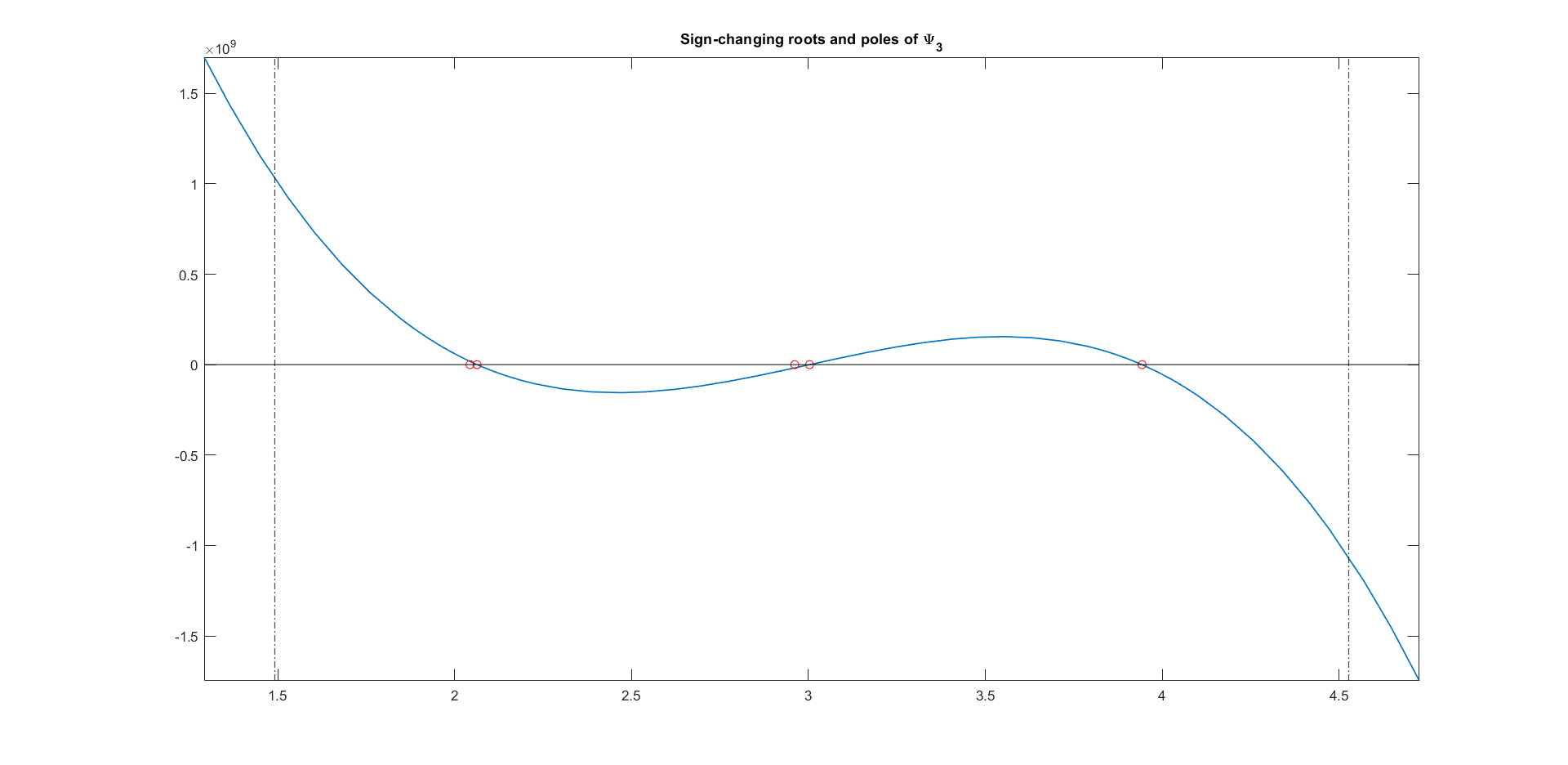
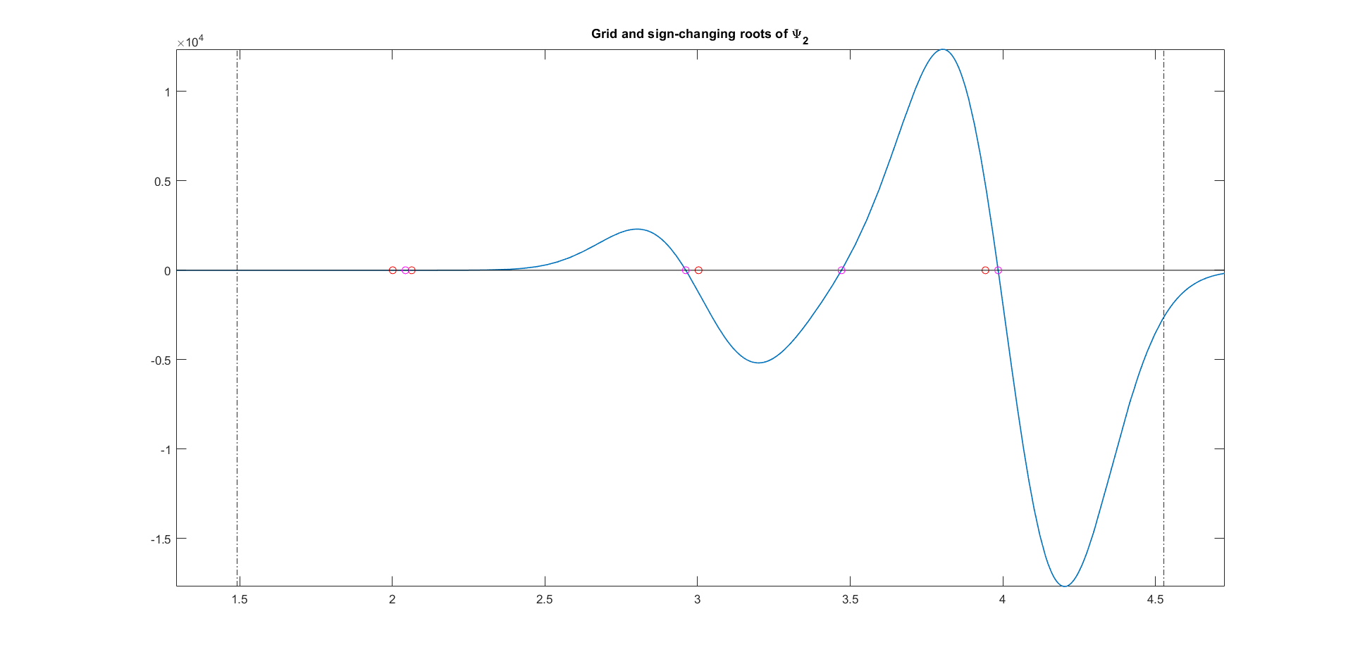
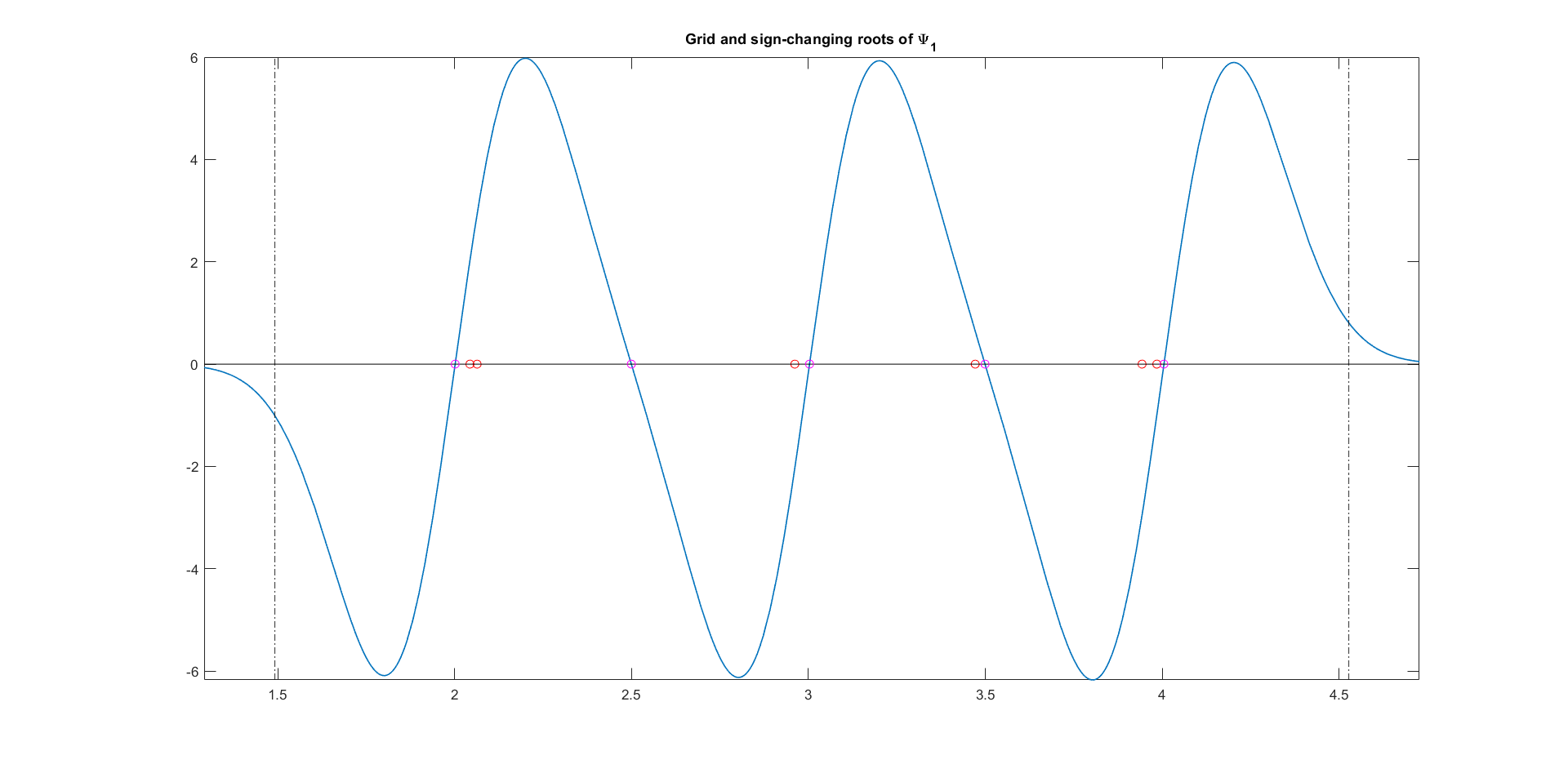
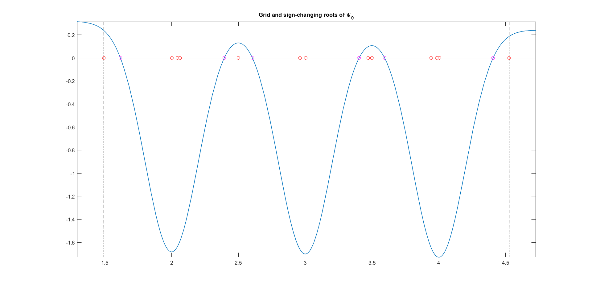
In the current example, the bounded interval was found to be equal to . The GBF functions along with their grids and sign-changing roots are displayed in fig. 4.
References
- [1] Luigi Ambrosio, Nicola Gigli, and Giuseppe Savaré. Gradient flows in metric spaces and in the space of probability measures. Lectures in Mathematics ETH Zürich. Birkhäuser Verlag, Basel, second edition, 2008.
- [2] Laura Aquilanti, Simone Cacace, Fabio Camilli, and Raul De Maio. A mean field games approach to cluster analysis. Appl. Math. Optim., 84(1):299–323, 2021.
- [3] Laura Aquilanti, Simone Cacace, Fabio Camilli, and Raul De Maio. A mean field games model for finite mixtures of Bernoulli and categorical distributions. J. Dyn. Games, 8(1):35–59, 2021.
- [4] Michel Coste, Tomás Lajous-Loaeza, Henri Lombardi, and Marie-Françoise Roy. Generalized budan–fourier theorem and virtual roots. Journal of Complexity, 21(4):479–486, 2005. Festschrift for the 70th Birthday of Arnold Schonhage.
- [5] Giorgio Dall’Aglio. Sugli estremi dei momenti delle funzioni di ripartizione doppia. Ann. Scuola Norm. Sup. Pisa Cl. Sci. (3), 10:35–74, 1956.
- [6] R. M. Dudley. Probabilities and metrics. Matematisk Institut, Aarhus Universitet, Aarhus, 1976. Convergence of laws on metric spaces, with a view to statistical testing, Lecture Notes Series, No. 45.
- [7] Paul Embrechts and Marius Hofert. A note on generalized inverses. Math. Methods Oper. Res., 77(3):423–432, 2013.
- [8] Brian S. Everitt, Sabine Landau, Morven Leese, and Daniel Stahl. Cluster analysis. Wiley Series in Probability and Statistics. John Wiley & Sons, Ltd., Chichester, fifth edition, 2011.
- [9] Sylvia Frühwirth-Schnatter. Finite mixture and Markov switching models. Springer Series in Statistics. Springer, New York, 2006.
- [10] André Galligo. Budan tables of real univariate polynomials. Journal of Symbolic Computation, 53:64–80, 2013.
- [11] Laureano Gonzalez-Vega, Henri Lombardi, and Louis Mahé. Virtual roots of real polynomials. Journal of Pure and Applied Algebra, 124(1-3):147 – 166, 1998. Cited by: 10; All Open Access, Bronze Open Access, Green Open Access.
- [12] Bernard Hanzon and Finbarr Holland. Non-negativity analysis for exponential-polynomial-trigonometric functions on . In Spectral theory, mathematical system theory, evolution equations, differential and difference equations, volume 221 of Oper. Theory Adv. Appl., pages 399–412. Birkhäuser/Springer Basel AG, Basel, 2012.
- [13] Anna Karapiperi, Michela Redivo-Zaglia, and Maria Rosaria Russo. Generalizations of sylvester’s determinantal identity, 2015.
- [14] Sergey Kasyanov. GaussElimination, 2022. MATLAB Central File Exchange. Version 1.0.0.
- [15] Geoffrey McLachlan and David Peel. Finite mixture models. Wiley Series in Probability and Statistics: Applied Probability and Statistics. Wiley-Interscience, New York, 2000.
- [16] J. Park and I. W. Sandberg. Universal approximation using radial-basis-function networks. Neural Computation, 3(2):246–257, 1991.
- [17] K. Pearson. Contribution to the mathematical theory of evolution. Philosophical Transactions A, 185:71–110, 1894.
- [18] G. Pólya. On the mean-value theorem corresponding to a given linear homogeneous differential equation. Trans. Amer. Math. Soc., 24(4):312–324, 1922.
- [19] Daniel Richardson. How to recognize zero. J. Symb. Comp., 24:627–645, 1997.
- [20] C. Ridders. A new algorithm for computing a single root of a real continuous function. IEEE Transactions on Circuits and Systems, 26(11):979–980, 1979.
- [21] Robert Ristroph. Pólya’s property and factorization—A short proof. Proc. Amer. Math. Soc., 31:631–632, 1972.
- [22] D. Hari Hara Santosh, P. Venkatesh, P. Poornesh, L. Narayana Rao, and N. Arun Kumar. Tracking multiple moving objects using gaussian mixture model. International Journal of Soft Computing and Engineering, 3(2):114 – 119, 2013.
- [23] Hugh Conor Sexton. Financial modelling with 2-EPT probability density functions. PhD Thesis, University College Cork, 2013.
- [24] D. M. Titterington, A. F. M. Smith, and U. E. Makov. Statistical analysis of finite mixture distributions. Wiley Series in Probability and Mathematical Statistics: Applied Probability and Statistics. John Wiley & Sons, Ltd., Chichester, 1985.
- [25] S. S. Vallander. Calculations of the Vasseršteĭn distance between probability distributions on the line. Teor. Verojatnost. i Primenen., 18:824–827, 1973.
- [26] Dong Yu and Li Deng. Automatic speech recognition. Signals and Communication Technology. Springer, London, 2015. A deep learning approach, With a foreword by Sadaoki Furui.