Lieb–Thirring inequalities on manifolds with constant negative curvature

Lieb–Thirring inequalities have important applications in mathematical physics, analysis, dynamical systems and attractors, to mention a few. A current state of the art of many aspects of the theory is presented in [9]. We mention here the celebrated paper by Lieb and Thirring [19], where such inequalities were studied for the questions of stability of matter.

In certain applications Lieb–Thirring inequalities are considered on a manifold. For example, on torus or sphere one has to impose the zero mean orthogonality condition, see [10], [13], [25], [12], [11]. Such inequalities are useful in the study of the dimension of attractors in theory of Navier-Stokes equation.

In this work we prove Lieb–Thirring inequalities on manifolds with negative constant curvature. Let $\mathbb{H}^{d}$, $d\geq 2$, be the upper half-space

$$\mathbb{H}^{d}=\{(x,y):\,x\in\mathbb{R}^{d-1},\,y\in\mathbb{R}_{+}\}$$

with the Poincare metric $ds^{2}=y^{-2}(dx^{2}+dy^{2})$. We consider the self-adjoint Laplace–Beltrami operator in $L^{2}\left(\mathbb{H}^{d},\frac{dx\,dy}{y^{d}}\right)$

$$-\Delta_{h}=-y^{d}\frac{\partial}{\partial y}\,y^{2-d}\,\frac{\partial}{\partial y}-y^{2}\,\sum_{n=1}^{d-1}\frac{\partial^{2}}{\partial x_{n}^{2}}.$$

(1.1)

The spectrum of the standard Laplacian

$$-\Delta=-\sum_{n=1}^{d}\frac{\partial^{2}}{\partial x_{n}^{2}}$$

acting in $L^{2}(\mathbb{R}^{d},dx)$ is absolutely continuous and covers the whole half-line $[0,\infty)$. By contrast, the spectrum of the Laplace operator (1.1) is continuous and covers the interval $[(d-1)^{2}/4,\infty)$, see for example [20], [21]  [16].

Denote by $L_{\gamma,d}^{\rm cl}$ the value

$$L_{\gamma,d}^{\rm cl}=\frac{1}{(2\pi)^{d}}\,\int_{\mathbb{R}^{d}}(1-|\xi|^{2})_{+}^{\gamma}\,d\xi=\frac{\Gamma(\gamma+1)}{(4\pi)^{d/2}\Gamma(\gamma+d/2+1)}.$$

Let $V=V(x)\geq 0$. The classical Lieb–Thirring inequality for a Schrödinger operator $-\Delta-V$ on $L^{2}(\mathbb{R}^{d})$ states

$${\rm Tr}\,\left(-\Delta-V\right)_{-}^{\gamma}\leq L_{\gamma,d}\int_{\mathbb{R}^{d}}V^{\gamma+d/2}\,dx.$$

In  [19] E.H. Lieb and W. Thirring proved that it holds for finite constants $L_{\gamma,d}$ as long as $\gamma>\max(0,1-d/2)$. In the case $d\geq 3,\,\gamma=0$ this bound is known as the Cwikel–Lieb–Rozenblum (CLR) inequality, see [3, 18, 23]. The second critical case $d=1,\gamma=1/2$ was settled by Weidl in [26]. The inequality is known to fail for $d=2,\gamma=0$. For a comprehensive treatment and references of the subject, see [9].

In this paper we study the spectrum of the Schrödinger operator

$$-\Delta_{h}-V,$$

(1.2)

acting in $L^{2}\left(\mathbb{H}^{d},\frac{dx\,dy}{y^{d}}\right)$ and obtain Lieb–Thirring inequalities for the discrete spectrum below $(d-1)^{2}/4$. It is convenient to denote the eigenvalues $\{\lambda_{k}\}$ of the operator (1.2) in terms of negative values $\{-\mu_{k}\}$, where

$$\lambda_{k}=\frac{(d-1)^{2}}{4}-\mu_{k}.$$

(1.3)

Let us denote by $R_{1,1}$ the value $R_{1,1}\leq 1.456\dots$ that was obtained in the recent paper [8] on the Lieb–Thirring inequality for a one-dimensional Schrödinger operator with an operator-valued potential.

The main result of the paper is the following:

In the next Section 2 we obtain a simple proof of the fact that the continuous spectrum of the Laplacian on hyperbolic space with curvature $-1$ covers the semi-axis $[(d-1)^{2}/4,\infty)$. In Section 3 we give the proof the main Theorem 1.1 and in Section 4 we obtain the dual inequality that could be used for estimates of the dimension of attractors in theory of the Navier–Stokes equation.

In Section 5 we apply Theorem 1.1 to derive an inequality on the number of eigenvalues below $\Lambda>0$ for Dirichlet Laplace–Beltrami operator on a domain $\Omega\subset\mathbb{H}^{d}$ of finite measure.

Assume that $\Omega\subset{\overline{\Omega}}\subset\mathbb{H}^{d}$ satisfies the inequality

$$|\Omega|_{h}=\int_{\Omega}\frac{dxdy}{y^{d}}<\infty.$$

We consider the Dirichlet eigenvalue problem for the Laplace–Beltrami operator $-\Delta_{h}$ in $L^{2}(\Omega,y^{-d}dxdy)$

$$-\Delta_{h}u=\lambda u,\qquad u\big|_{(x,y)\in\partial\Omega}=0.$$

(1.5)

The spectrum of this operator is discrete and we denote by $\{\lambda_{k}\}$ its eigenvalues. Such eigenvalues satisfy the inequality

$$\lambda_{k}>\frac{(d-1)^{2}}{4}.$$

Similarly to (1.3) it is convenient to introduce number $\nu_{k}$ such that

$$\lambda_{k}=\frac{(d-1)^{2}}{4}+\nu_{k}$$

and study the counting function $\mathcal{N}(\Lambda)$ of the spectrum

$$\mathcal{N}(\Lambda)=\#\{k:\,\nu_{k}<\Lambda\},\qquad\Lambda>0.$$

The inequality (1.6) is a Pólya type inequality [22] for manifolds with constant negative curvature, where, we believe, the constant is not sharp.

In Section 6 we consider the special case of Theorem 1.2, where $\Omega=\widetilde{\Omega}\times(a,b)$, $\widetilde{\Omega}\subset\mathbb{R}^{d-1}$, is a domain of finite Lebesgue measure and $0<a<b\leq\infty$. This additional structure of $\Omega$ allows us to obtain a better constant than the constant that could be derived from Theorem 1.1 in the case $1/2\leq\gamma<1$, see Theorem 6.1. Unfortunately it does not imply the improvement of the constant found in Theorem 1.2.

Finally in Section 7 we give an example of a domain in $\mathbb{H}^{2}$ supporting the conjecture 1 using numerics.

In [20] the author gives a simple proof of the fact that the continuous spectrum of the operator $-\Delta_{h}$ in dimension two coincides with the interval $[1/4,\infty)$ by using the Cauchy-Schwarz inequality. Besides, he gives a more complicated proof of the fact that in the case of $\mathbb{H}^{d}$, $d>2$ the continuous spectrum fills the half-axis $[(d-1)^{2}/4,\infty)$.

In this section we present a simple proof of the following well-known fact.

In order to prove Theorem 1.1 we need to recall some results on 1D Schrödinger operators with operator-valued potentials.

If $\gamma=1/2$ then the constant $L_{\gamma=1/2,1}=2L_{1/2,1}^{\rm cl}$ and it is sharp. This was obtained in [6] and from this one immediately obtains that $L_{\gamma,1}\leq 2L_{\gamma,1}^{\rm cl}$ with $1/2\leq\gamma<1$. (For the scalar case the sharp constant in the case $\gamma=1/2$ was obtained in [7].

If $\gamma=1$ then the sharp constant is unknown and the best known constant for some years was refereed to [4] (see also [5]). It is only recently this constant was improved in the paper [8], where the authors found that $L_{1,1}\leq R_{1,1}L_{1,1}^{\rm cl}$ with $R_{1,1}\leq 1.456\dots.$ This leads to the estimate $L_{\gamma,1}\leq R_{1,1}L_{\gamma,1}^{\rm cl}$ with $1\leq\gamma<3/2$.

Finally for any $\gamma\geq 3/2$ the above Proposition was proved in [15] and in this case we have sharp constants $L_{\gamma,1}=L_{\gamma,1}^{\rm cl}$.

In all cases the authors first obtained inequalities for $\gamma=1/2,1$ and $3/2$ that were afterwards extended to arbitrary $\gamma$’s using lifting argument found by Aizenman and Lieb [1].

Let us consider the quadratic form of the operator (1.1)

$$(-\Delta_{h}u,u)=\int_{\mathbb{H}^{n}}y^{2-d}\,\left(|\partial_{y}u|^{2}+\sum_{n=1}^{d-1}|\partial_{x_{n}}u|^{2}\right)\,dx\,dy.$$

Applying the exponential change of variables that was introduced in the previous section we reduce the problem to the study of the spectrum defined by the form in $L^{2}(\mathbb{R}^{d})$

$$\int_{\mathbb{R}^{d}}\left(|v_{t}^{\prime}|^{2}+e^{2t}\sum_{n=1}^{d-1}|\partial_{x_{n}}v|^{2}-V(x,e^{t})|v|^{2}\right)\,dxdt=-\mu\,\int_{\mathbb{R}^{d}}|v|^{2}\,dxdt.$$

Consider an orthonormal set of function $\{u_{m}\}_{m=1}^{M}$ in $L^{2}(\mathbb{H}^{d},y^{-d}\,dxdy)$. Then using the exponential change

$$y=e^{t},\qquad u_{m}=e^{(d-1)t/2}\,v_{m}$$

we find

$$\delta_{m,l}=\int_{\mathbb{H}^{d}}u_{m}{\overline{u}_{l}}\frac{dxdy}{y^{d}}=\int_{\mathbb{R}^{d}}v_{m}{\overline{v}_{l}}\,dxdt.$$

Namely, this shows that if the functions $\{u_{m}\}_{m=1}^{M}$ are orthonormal in $L^{2}(\mathbb{H}^{d},y^{-d}\,dxdy)$ then the functions $\{v_{m}\}_{m=1}^{M}$ are orthonormal in $L^{2}(\mathbb{R}^{d})$.

Assuming $\gamma=1$ we obtain

$$\sum_{m=1}^{M}\int_{\mathbb{R}^{d}}\left(|\partial_{t}v_{m}|^{2}+e^{2t}\,\sum_{n=1}^{d-1}|\partial_{x_{n}}v_{m}|^{2}-V(x,e^{t})|v_{m}|^{2}\right)\,dxdt\\ \geq-\sum_{m}\mu_{m}\geq-L_{1,d}\,\int_{\mathbb{R}^{d}}V(x,e^{t})^{1+d/2}\,dxdt.$$

Assume that $M=1$ and $u\in H^{1}(\mathbb{H}^{d},y^{-d}dxdy)$ and denote

$$\|u\|=\left(\int_{\mathbb{H}^{d}}|u|^{2}\,\frac{dxdy}{y^{d}}\right)^{1/2}.$$

Then

Let $\Omega\subset{\overline{\Omega}}\subset\mathbb{H}^{d}$ be a domain of finite measure $|\Omega|_{h}$ and let us introduce the following potential

$$V=\begin{cases}1,&(x,y)\in\Omega,\\ -\infty,&(x,y)\not\in\Omega.\end{cases}$$

Then the problem of the study of the counting function $\mathcal{N}(\Lambda)$ is reduced to the study of the number of the negative eigenvalues of the operator in $L^{2}(\mathbb{H}^{d},y^{-d}dxdy)$.

$$-\Delta_{h}-(d-1)^{2}/4-\Lambda V,$$

because the above operator is unitary equivalent to the operator

$$-\Delta_{h}-(d-1)^{2}/4-\Lambda$$

in $L^{2}(\Omega,y^{-d}dxdy)$ with Dirichlet boundary conditions. This number coincides with the number of $k$’s such that $\nu_{k}<\Lambda$. Therefore using the variational principle and applying Theorem 1.1 with $\gamma=1$ we find

$$\sum_{k}(\nu_{k}-\Lambda)_{-}=\sum_{k}(\Lambda-\nu_{k})_{+}\leq L_{1,d}\,\Lambda^{1+d/2}\,\int_{\Omega}\frac{dxdy}{y^{d}}=L_{1,d}\,\Lambda^{1+d/2}\,|\Omega|_{h}.$$

Then for any $\Upsilon>\Lambda$

$$\mathcal{N}(\Lambda)\leq\frac{1}{\Upsilon-\Lambda}\,\sum_{k}(\Upsilon-\nu_{k})_{+}\leq L_{1,d}\,\frac{\Upsilon^{1+d/2}}{\Upsilon-\Lambda}\,|\Omega|_{h}.$$

Minimising the right hand side of the latter inequality we find

$$\Upsilon=\Lambda\frac{1+d/2}{d/2}$$

and thus

$$\mathcal{N}(\Lambda)\leq\left(1+\frac{d}{2}\right)\left(1+\frac{2}{d}\right)^{d/2}\,R_{1,1}\,L_{1,d}^{\rm cl}\,|\Omega|_{h}\,\Lambda^{d/2}.$$

(5.1)

This concludes the proof of Theorem 1.2.

Similarly to Section 5 we can use the inequality (6.2) for estimating the counting function $\mathcal{N}(\Lambda)$ for spectrum of the Dirichlet Laplacian (1.1) in domain with the product structure. Indeed, for any $\Upsilon>\Lambda$

$$\mathcal{N}(\Lambda)\leq\frac{1}{(\Upsilon-\Lambda)^{1/2}}\,\sum_{\ell,k=1}^{\infty}(\Upsilon-\nu_{\ell k})_{+}^{1/2}\leq 2L_{1/2,d}^{\rm cl}\,\frac{\Upsilon^{(d+1)/2}}{(\Upsilon-\Lambda)^{1/2}}\,|\Omega|_{h}.$$

Minimising the right hand side of the latter inequality we find $\Upsilon=\Lambda\frac{1+d}{d}$ and thus

$$\mathcal{N}(\Lambda)\leq\left(\frac{d+1}{d}\right)^{(d+1)/2}\,\sqrt{d}\,2\,L_{1/2,d}^{\rm cl}\,|\Omega|_{h}\,\Lambda^{d/2}.$$

(6.3)

However, the ratio of the constants (6.3) and (5.1) is greater than one and therefore Theorem 6.1 does not imply any improvement for the inequality (5.1).

Let $d=2$ and let

$$\Omega=(0,\pi)\times(e^{-1},e)=\left\{(x,y):\,x\in(0,\pi),\,y\in(e^{-1},e)\right\}$$

with

$$|\Omega|_{h}=\pi(e-e^{-1}).$$

Consider the Dirichlet Laplacian $-\Delta_{h}$ in $L^{2}(\Omega,y^{-2}dxdy)$ defined in (1.1). Using the notations from Section 6 we have $\alpha=-1$, $\beta=1$. Obviuosly the eigenvalues of the problem

$$-\partial^{2}_{x}\varphi=\varkappa\varphi,\quad\varphi\big|_{x=0,\pi}=0$$

are $\varkappa_{\ell}=\ell^{2}$.

The arguments from Section 6 imply that the problem is reduced to the study of the eigenvalues $\nu_{\ell k}$ satisfying the equation

$$-\partial_{t}^{2}\,\psi_{\ell k}(t)+e^{2t}\,\ell^{2}\,\psi_{\ell k}(t)=\nu_{\ell k}\,\psi_{\ell k}(t),\qquad\psi_{\ell k}(t)\big|_{t=-1,1}=0.$$

(7.1)

Now comes numerics to prove the following Pólya type inequality:

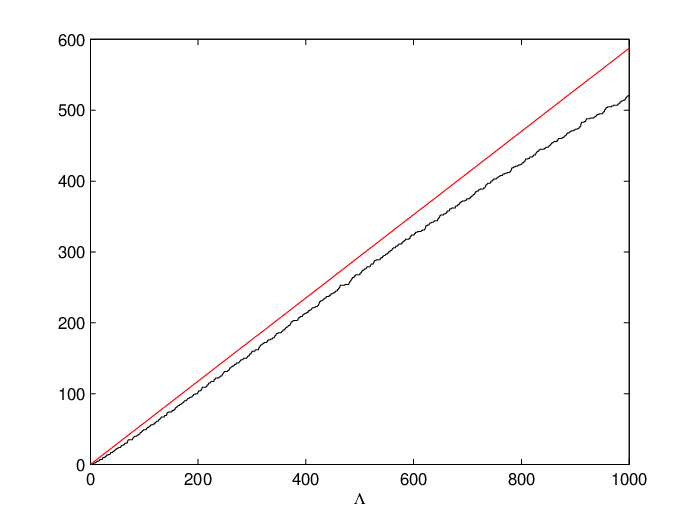
$$\mathcal{N}(\Lambda)=\#\{\ell,k:\,\nu_{\ell k}<\Lambda\}\leq(2\pi)^{-2}\int_{0}^{\pi}\int_{-1}^{1}\int_{\xi_{2}^{2}+e^{2t}\xi_{1}^{2}<\Lambda}d\xi_{1}d\xi_{2}dtdx\\ =(2\pi)^{-2}\pi\Lambda\int_{-1}^{1}e^{-t}\int_{\xi_{1}^{2}+\xi_{2}^{2}<1}d\xi_{2}d\xi_{1}=\frac{1}{4}\Lambda\left(e-e^{-1}\right)=L^{\rm cl}_{0,2}\Lambda|\Omega|_{h}.$$

Let us say a few words about the calculations of the eigenvalues of the collection of problems (7.1). We use the Chebyshev differentiation matrix [24] for the spectral approximation of the derivative (and this matrix squared for the second derivative) for the numerical solution of the eigenvalue problems (7.1) (we observe that the potentials are analytic). We have used matrices of order $400\times 400$. The accuracy is tested against the problem (7.1) with $l=0$, so that the corresponding eigenvalues $n^{2}\cdot\frac{4}{\pi^{2}}$ are computed for $n=1,\dots,200$ with correct 14 decimal places. We therefore reasonably expect that the accuracy is of the similar order for $\ell\geq 1$.

We set $\Lambda\leq 1000$. Then to calculate $\mathcal{N}(\Lambda)$ it is enough to limit $l\leq 50$, since the first eigenvalue of  (7.1) with $l=50$ is already greater than $1000$. The eigenvalues $\nu_{\ell k}$ are of the order $k^{2}\cdot\frac{4}{\pi^{2}}$ and the therefore the length $[1:200]$ of each the sequence of eigenvalues $\nu_{\ell k}$ taken into account for each fixed $\ell\leq 50$ is also more than enough for $\Lambda\leq 1000$.

Acknowledgements: The authors would like to thank N. A. Zaitsev for his help and advice concerning the computer calculations of the eigenvalues of the Sturm–Liouville problems (7.1).

The work of A.I. was supported by Moscow Center for Fundamental and Applied Mathematics, Agreement with the Ministry of Science and Higher Education of the Russian Federation, No. 075-15-2022-283. AL was supported by the Ministry of Science and Higher Education of the Russian Federation, (Agreement 075-10-2021-093, Project MTH-RND-2124).

References

• [1] M. Aizenman and E.H. Lieb, On semi-classical bounds for eigenvalues of Schrödinger operators. Phys. Lett. 66A (1978), 427–429.
• [2] F.A. Berezin, Convex functions of operators. Mat. Sb., 88 (130), 268–276. English translation in Math. USSR-Sb., 17 (2), (1972), 269–277.
• [3] M. Cwikel, Weak type estimates for singular values and the number of bound states of Schrödinger operators. Trans. AMS, 224, (1977), 93–100.
• [4] J. Dolbeault, A. Laptev, and M. Loss, Lieb–Thirring inequalities with improved constants. J. European Math. Soc. 10:4 (2008), 1121–1126.
• [5] A. Eden and C. Foias, A simple proof of the generalized Lieb–Thirring inequalities in one space dimension. J. Math. Anal. Appl. 162 (1991), 250–254.
• [6] D. Hundertmark, A. Laptev, T. Weidl, New bounds on the Lieb-Thirring constants. Invent. Math., 140 (2000), 693–704.
• [7] D. Hundertmark, E.H. Lieb, L.E. Thomas, A sharp bound for an eigenvalue moment of the one-dimensional Schrödinger operator. Adv. Theor. Math. Phys., 2 (1998), 719–731.
• [8] R.L. Frank, D. Hundertmark, M. Jex, P.T. Nam, The Lieb–Thirring inequality revisited. J. European Math. Soc., 23 (2021), 2583–2600.
• [9] R.L. Frank, A. Laptev, and T. Weidl, Schrödinger Operators: Eigenvalues and Lieb–Thirring Inequalities. (Cambridge Studies in Advanced Mathematics 200). Cambridge: Cambridge University Press, 2022.
• [10] A. Ilyin, A. Laptev, M. Loss, and S. Zelik, One-dimensional interpolation inequalities, Carlson-Landau inequalities, and magnetic Schrodinger operators. Int. Math. Res. Not. IMRN (2016) 2016:4, 1190–1222.
• [11] A.A. Ilyin and A.A. Laptev, Magnetic Lieb–Thirring inequality for periodic functions. Uspekhi Mat. Nauk 75:4 (2020), 207–208; English transl. in Russian Math. Surveys 75:4 (2020), 779–781.
• [12] A.A. Ilyin and A.A. Laptev, Lieb-Thirring inequalities on the torus. Mat. Sb. 207:10 (2016), 56–79; English transl. in Sb. Math. 207:9-10 (2016).
• [13] A. Ilyin, A. Laptev, and S. Zelik, Lieb–Thirring constant on the sphere and on the torus. J. Func. Anal. 279 (2020) 108784.
• [14] A. Laptev, Dirichlet and Neumann eigenvalue problems on domains in Euclidean spaces. J. Funct. Anal., 151 (2), (1997), 531–545..
• [15] A. Laptev and T. Weidl, Sharp Lieb–Thirring inequalities in high dimensions. Acta Math., 184 (2000), 87–111.
• [16] P. Lax, R.S. Phillips, The asymptotic distribution of lattice points in Euclidean and non-Euclidean spaces. JFA, 46 (1982), 280–350.
• [17] P. Li and S.T. Yau, On the Schrödinger equation and the eigenvalue problem. Comm. Math. Phys., 88 (3) (1983), 309–318.
• [18] E.H. Lieb, Bounds on the eigenvalues of the Laplace and Schrödinger operators. Bull. Amer. Math. Soc. 82 (1976), 751–753. (1976). See also: The number of bound states of one body Schrödinger operators and the Weyl problem. Proc. A.M.S. Symp. Pure Math. 36 (1980), 241–252.
• [19] E.H. Lieb, W. Thirring, Inequalities for the moments of the eigenvalues of the Schrödinger Hamiltonian and their relation to Sobolev inequalities. Studies in Math. Phys., Essays in Honor of Valentine Bargmann., Princeton (1976), 269–303.
• [20] H.P. McKean, An upper bound to the Spectrum of Δ\Delta on a manifold of negative curvature. J. Differential Geometry 4 (1970), 359–366.
• [21] P.A. Perry, The Laplace Operator on a Hyperbolic Manifold I. Spectral and Scattering Theory. JFA 75 (1987), 161–187.
• [22] G. Pólya, On the eigenvalues of vibrating membranes. Proc. London Math. Soc. 11 (1961), 419–433.
• [23] G.V. Rozenblum, Distribution of the discrete spectrum of singular differential operators. Dokl. AN SSSR, 202 (1972), 1012–1015, Izv. VUZov, Matematika, 1 (1976), 75–86.
• [24] L.N. Trefethen, Spectral methods in Matlab. Philadelphia, SIAM, 2000.
• [25] S.V. Zelik and A.A. Ilyin, Green’s function asymptotics and sharp interpolation inequalities. Uspekhi Mat. Nauk 69:2 (2014), 23–76; English transl. in Russian Math. Surveys 69:2 (2014).
• [26] T. Weidl, On the Lieb-Thirring constants Lγ,1L_{\gamma,1} for γ≥1/2\gamma\geq 1/2. Comm. Math. Phys. 178 (1996), 135–146.